Article

Parallel Cooperative Coevolutionary Grey Wolf Optimizer for Path Planning Problem of Unmanned Aerial Vehicles

1
Research Laboratory in Automatic Control (LARA), National Engineering School of Tunis (ENIT), University of Tunis El Manar, Tunis 1002, Tunisia
2
Control and Instrumentation Engineering Department, King Fahd University of Petroleum & Minerals, Dhahran 31261, Saudi Arabia
3
Interdisciplinary Research Center (lRC) for Renewable Energy and Power Systems, King Fahd University of Petroleum & Minerals, Dhahran 31261, Saudi Arabia
4
College of Engineering at Wadi Addawaser, Prince Sattam Bin Abdulaziz University, Al-Kharj 11911, Saudi Arabia
5
High Institute of Industrial Systems of Gabes (ISSIG), University of Gabes, Gabes 6011, Tunisia
*
Author to whom correspondence should be addressed.
Sensors 2022, 22(5), 1826; https://doi.org/10.3390/s22051826
Submission received: 30 December 2021 / Revised: 17 February 2022 / Accepted: 21 February 2022 / Published: 25 February 2022
(This article belongs to the Special Issue Sensors and Algorithms for Autonomous Navigation of Aircraft)

Abstract

:
The path planning of Unmanned Aerial Vehicles (UAVs) is a complex and hard task that can be formulated as a Large-Scale Global Optimization (LSGO) problem. A higher partition of the flight environment leads to an increase in route’s accuracy but at the expense of greater planning complexity. In this paper, a new Parallel Cooperative Coevolutionary Grey Wolf Optimizer (PCCGWO) is proposed to solve such a planning problem. The proposed PCCGWO metaheuristic applies cooperative coevolutionary concepts to ensure an efficient partition of the original search space into multiple sub-spaces with reduced dimensions. The decomposition of the decision variables vector into several sub-components is achieved and multi-swarms are created from the initial population. Each sub-swarm is then assigned to optimize a part of the LSGO problem. To form the complete solution, the representatives from each sub-swarm are combined. To reduce the computation time, an efficient parallel master-slave model is introduced in the proposed parameters-free PCCGWO. The master will be responsible for decomposing the original problem and constructing the context vector which contains the complete solution. Each slave is designed to evolve a sub-component and will send the best individual as its representative to the master after each evolutionary cycle. Demonstrative results show the effectiveness and superiority of the proposed PCCGWO-based planning technique in terms of several metrics of performance and nonparametric statistical analyses. These results show that the increase in the number of slaves leads to a more efficient result as well as a further improved computational time.

1. Introduction

Unmanned Aerial Vehicles (UAVs) have recently become an interesting research topic, due to their strong survivability in many activities such as agricultural, commercial, military, and civilian [1,2,3,4]. To achieve repetitive and hard missions in dangerous environments, path planning is a key task in the UAVs’ control system [5,6,7,8]. The purpose of drones’ path planning is not only to find a collision-free path to reach the target but also to select an optimal flyable path that minimizes some critical goals.
The complexity and hardness of UAVs’ path planning problems are increased due to the increase in optimization factors such as UAV restrictions and environmental restrictions. To deal with this complexity, researchers have gradually moved from using the conventional to non-conventional planning approaches considered more effective. In study [9], the authors proposed an improved Particle Swarm Optimization (PSO) algorithm, by introducing the competition strategy formalism, to solve the 3D path planning for fixed-wing UAVs. In study [10], Jamshidi et al. described a CAN bus-based implementation of an asynchronous distributed multi-master parallel Genetic Algorithm (GA) and PSO metaheuristics to improve the performance and computational time of the UAV path planning task. A path planning approach based on the Water Cycle Algorithm (WCA) to find the optimal or near-optimal path avoiding all obstacles in 2D environments is proposed in [11]. The authors in [12] proposed a comprehensively improved particle swarm optimization to enhance the optimality and rapidity of automatic path planners for autonomous UAV formation systems. In studies [13,14], the authors proposed a new methodology to discover the UAV optimal path planning based on a Multiobjective Multi-Verse Algorithm (MOMVA). The authors in [15] proposed a novel approach to solve the UAV path planning based on a Grey Wolf Optimizer (GWO) by proper choice of optimization models such as the objective function for targets and constraints for obstacles’ avoidance. In study [16], another GWO-based method is proposed to solve the UAV path planning problem formulated as a hard optimization problem under operational constraints in terms of path shortness and smoothness as well as avoidance of obstacles. In the same work, the performance of the proposed parameters-free GWO algorithm is compared to other homologous metaheuristics such as the Crow Search Algorithm (CSA), Differential Evolution (DE), Salp Swarm Algorithm (SSA), and others. In study [17], the researchers proposed an improved Adaptive Grey Wolf Optimization (AGWO) algorithm to solve the 3D path planning of UAVs in a complex environment of material delivery in earthquake-stricken areas. Such an algorithm runs with an adaptive convergence factor and updated positions of the search agents. In study [18], a multi-population Chaotic Grey Wolf Optimizer (CGWO)-based method is investigated to solve the 3D UAVs’ cooperative path planning problem. A chaotic search strategy is introduced in this algorithm to improve the exploration/exploitation capabilities of the search behavior. In study [19], Kumar et al. described a modified version of the conventional GWO algorithm (MGWO) to design and optimize suitable paths for autonomous robots.
Such an above study was carried out to arouse the interest in the GWO algorithm widely applied in the field of UAVs’ path planning. The advantages in terms of simplicity of software implementation, reduced number of the algorithm’s control parameters, and convergence fastness make the GWO one of the most extensively used algorithms in the past three years [20,21,22,23]. The increased number of scientific publications on this topic explains the effectiveness of such a stochastic and parameters-free algorithm for solving various optimization problems. However, it should be pointed out that the GWO algorithm is often unable to escape trapping in local minima and presents a premature convergence, especially for the Large-Scale Global Optimization (LSGO) problems. Like most metaheuristics algorithms, the GWO suffers from the “dimensionality curse” and often fails to solve these hard optimization problems [17]. Thus, a practical implementation of such a metaheuristic algorithm presents a challenge in real-world applications due to its prohibitive computational time and weakness concerning an increased number of decision variables of optimization. Although the cited works [15,16,17,18,19] have been developed to solve the UAVs’ path planning problem based on a GWO algorithm, most of them formulated the planning problem with a small number of decision variables. Since the real-world planning tasks are considered LSGO problems, the quantity of computation increases strongly with the increase of the search space dimension, which implies a high probability of converging towards the local optimum [24]. These limits present a serious challenge for the real-time implementation of such an algorithm to design flyable and collision-free UAV paths.
To overcome these difficulties, the cooperative co-evolutionary concept of optimization seems an interesting idea to further improve the use of GWO algorithms for LSGO problems, particularly in UAVs’ path planning formalism. Such a design approach presents an effective tools’ panoply for solving hard problems thanks to its decomposition of optimization problems into smaller-dimension sub-components. It is a “divide and conquer” strategy initially proposed by Potter and De Jong in [25]. In the literature, the cooperative coevolutionary approach has been successfully applied for various optimization algorithms such as GA [26], PSO [27], DE [28], Simulated Annealing (SA) [29], Ant Colony Optimization (ACO) [30,31], Firefly algorithm [32], and many others. On the other hand, a large quantity of evaluation, due to the large number of problem decision variables, also implies an increased prohibitive computation time. However, online implementation of the standard GWO algorithm for a real-time path planning problem can be failed or at least become ineffective to achieve the desired performance of planning. To overcome this computation constraint, the parallelization concept can be introduced to reduce the complexity of the planning tasks and further increase the computational time of the investigated GWO algorithm.
Over the past decades, there has been a growing interest in the parallelization of metaheuristics algorithms [33,34,35,36,37,38,39,40]. Such advanced mechanisms for computation accelerating and enhancement greatly contribute to the success of metaheuristics for solving hard and large-scale optimization problems. In the literature, many types of metaheuristics algorithms have been recently parallelized based on different architectures and hardware resources. The Graphics Processing Units (GPUs) and multi-core Central Processing Units (CPUs)-based techniques are the most extensively proposed approaches. In study [33], a model of a vector parallel’s Ant Colony Optimization (ACO) algorithm is proposed using a multi-core SIMD CPU architecture. Each ant is mapped with a CPU core and the tour construction is accelerated by vector instructions. In study [34], a parallel heterogeneous ensemble feature selection method based on the three genetic (GA), particle swarm (PSO), and grey wolf (GWO) metaheuristics is proposed to enhance the performance of machine learning formalism. The hardware implementation is achieved on a multi-core CPU with GPU. In study [35], a parallel GA algorithm on GPU is investigated and compared to a sequential execution on CPU for wireless sensor data acquisition using a team of unmanned aerial vehicles. In study [36], an island model-based parallel GA is proposed and implemented on a GPU for solving the unequal area facility layout problem. In study [37], a comprehensive survey on parallel PSO algorithms is presented along with their strategies and applications. Several platforms and models, mainly the CPU- and GPU-based parallelization strategies, have been described and discussed. Another comprehensive survey on the parallel implementation of metaheuristics but within a multi-objective evolutionary framework is presented in [38]. An up-to-date review of methods and key contributions to such a research field are described. Other various techniques and strategies of metaheuristics parallelization are described and discussed in [39,40].
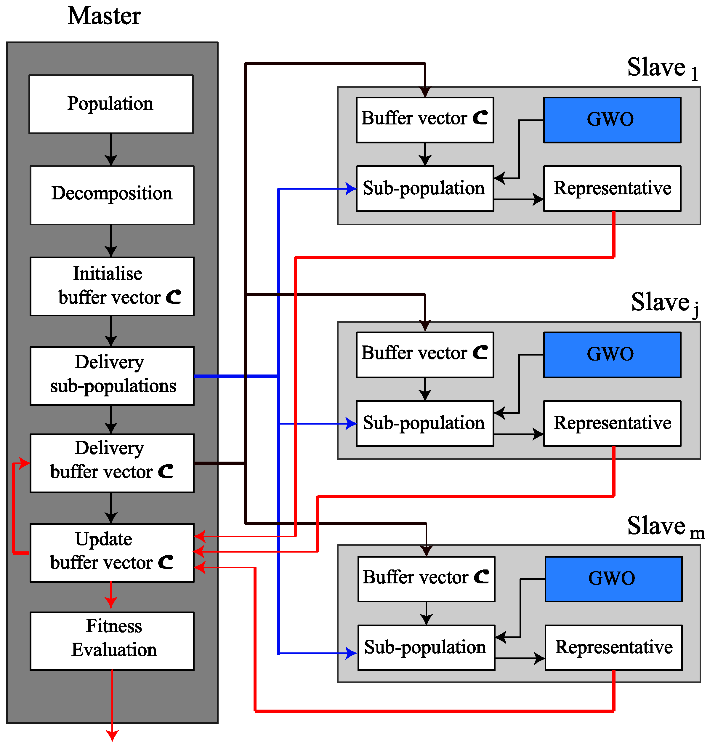
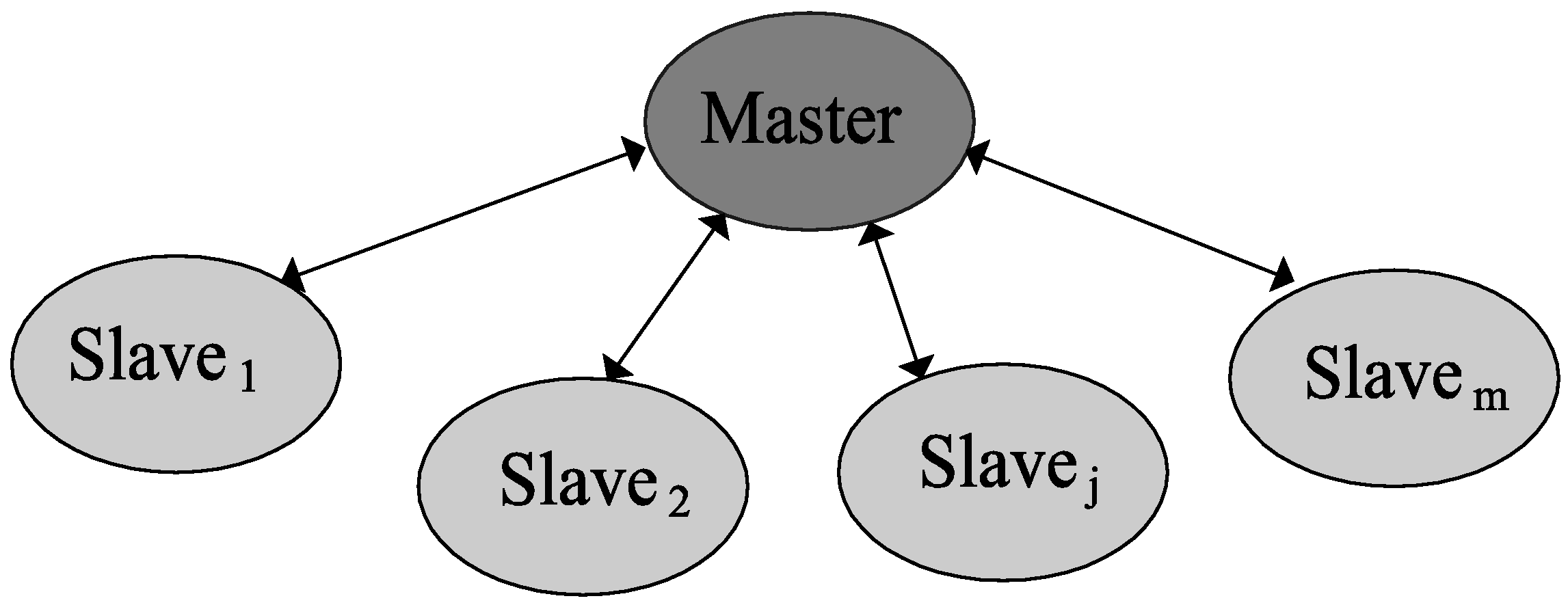
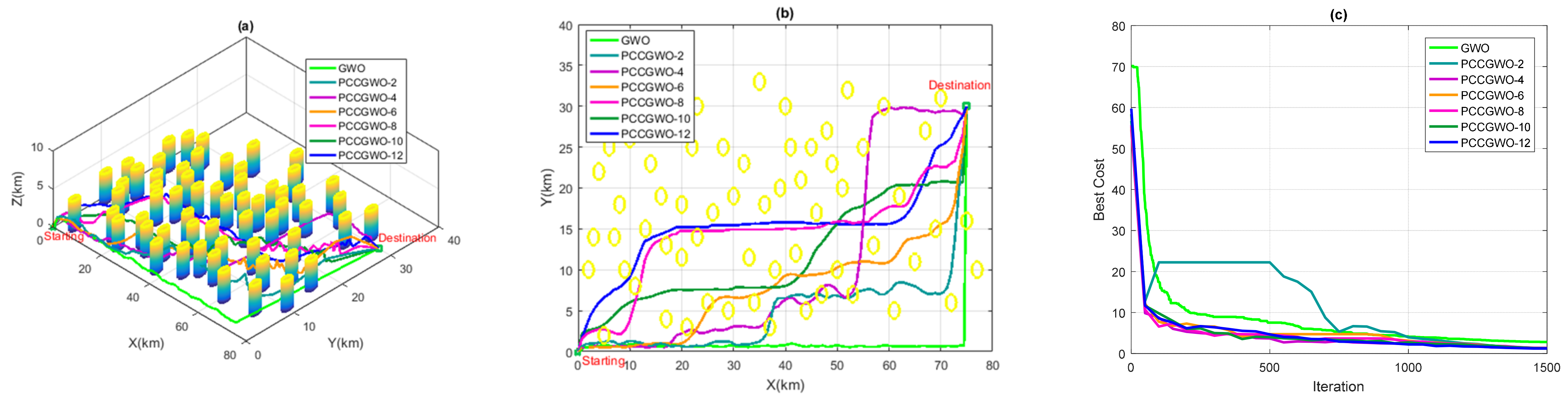
Based on these observations, the idea of using the parameters-free GWO algorithm, improved with the two concepts of cooperative coevolutionary and parallel computing, remains a promising and encouraging solution to solve the UAVs’ path planning problems. Indeed, in real-world UAVs’ planning applications, the most suited planners are those with fewer tuning of the effective parameters and a high fastness of the computation processing concerning the dynamics of navigation and software/hardware specifications of embedded control units. High performances in terms of computation speediness, shorter and collision-free flyable paths are always requested and recommended. In this work, a new Parallel Cooperative Coevolutionary Grey Wolf Optimizer (PCCGWO) is proposed and successfully applied in solving the UAVs’ path planning problem over large benchmarks and instances of navigation. Such an improved GWO algorithm combines the cooperative coevolutionary and parallelization mechanisms to ensure an efficient partition of the original large-scale search space into multiple sub-spaces with reduced dimensions. The decomposition of the decision variables vector into several sub-components is achieved and multi-swarms are created from the initial population to be later assigned to optimize a part of the path planning procedure formulated as an LSGO problem. The main contributions of this paper are summarized as follows: (1) an intelligent and efficient path planning strategy is elaborated to guide UAV drones to reach the destination position while avoiding a high number of obstacles and threats. (2) A novel parameters-free PCCGWO algorithm based on an efficient parallelization master-slave mechanism is proposed and successfully applied to solve the UAVs’ path planning problem over several flight scenarios. (3) A nonparametric statistical analysis in the sense of Friedman and post hoc tests is carried out to show the effectiveness and superiority of the proposed PCCGWO-based path planning approach.
The remainder of this paper is organized as follows. In Section 2, the path planning problem for unmanned aerial vehicles is formulated as a constrained large-scale optimization problem. Section 3 presents the proposed parallel cooperative coevolutionary grey wolf optimizer as well as its designed master-slave architecture. A pseudo-code of the proposed PCCGWO algorithm is given to solve the formulated UAVs’ path planning problem. In 
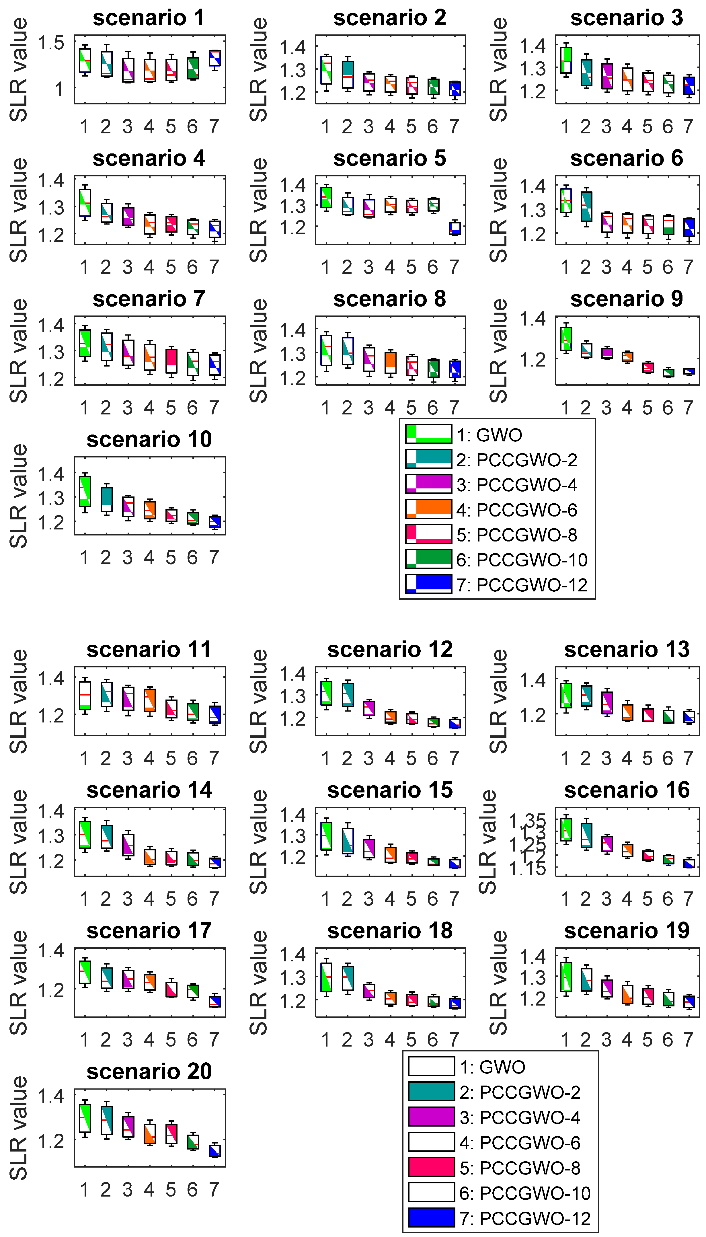
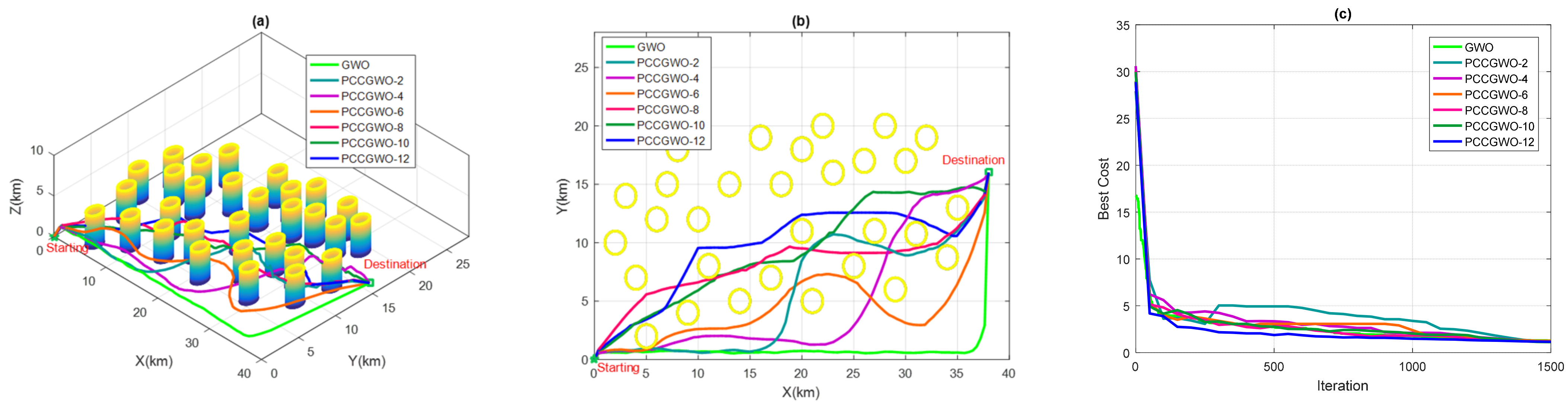
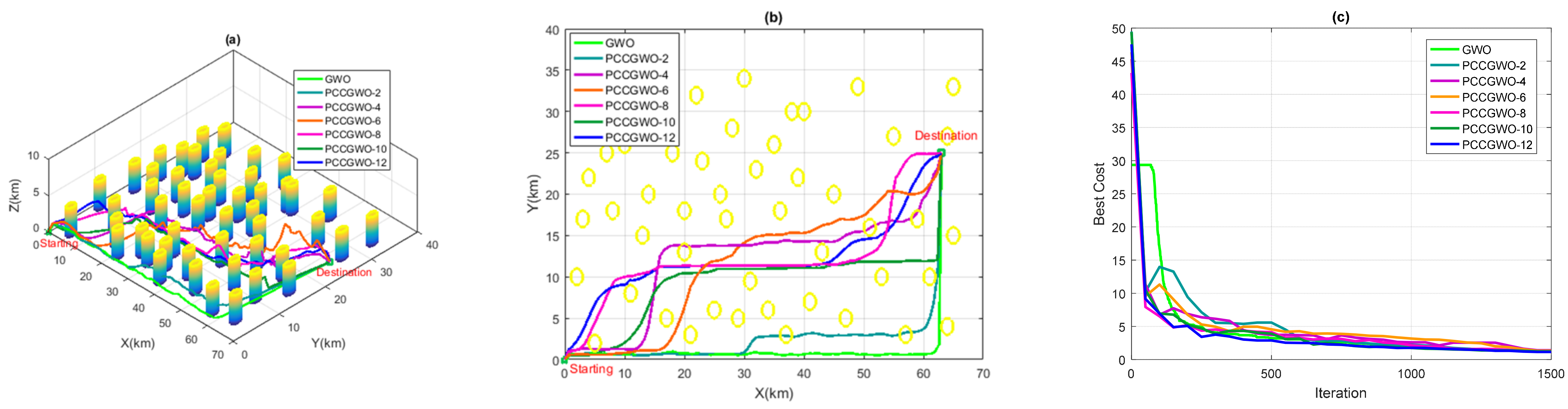
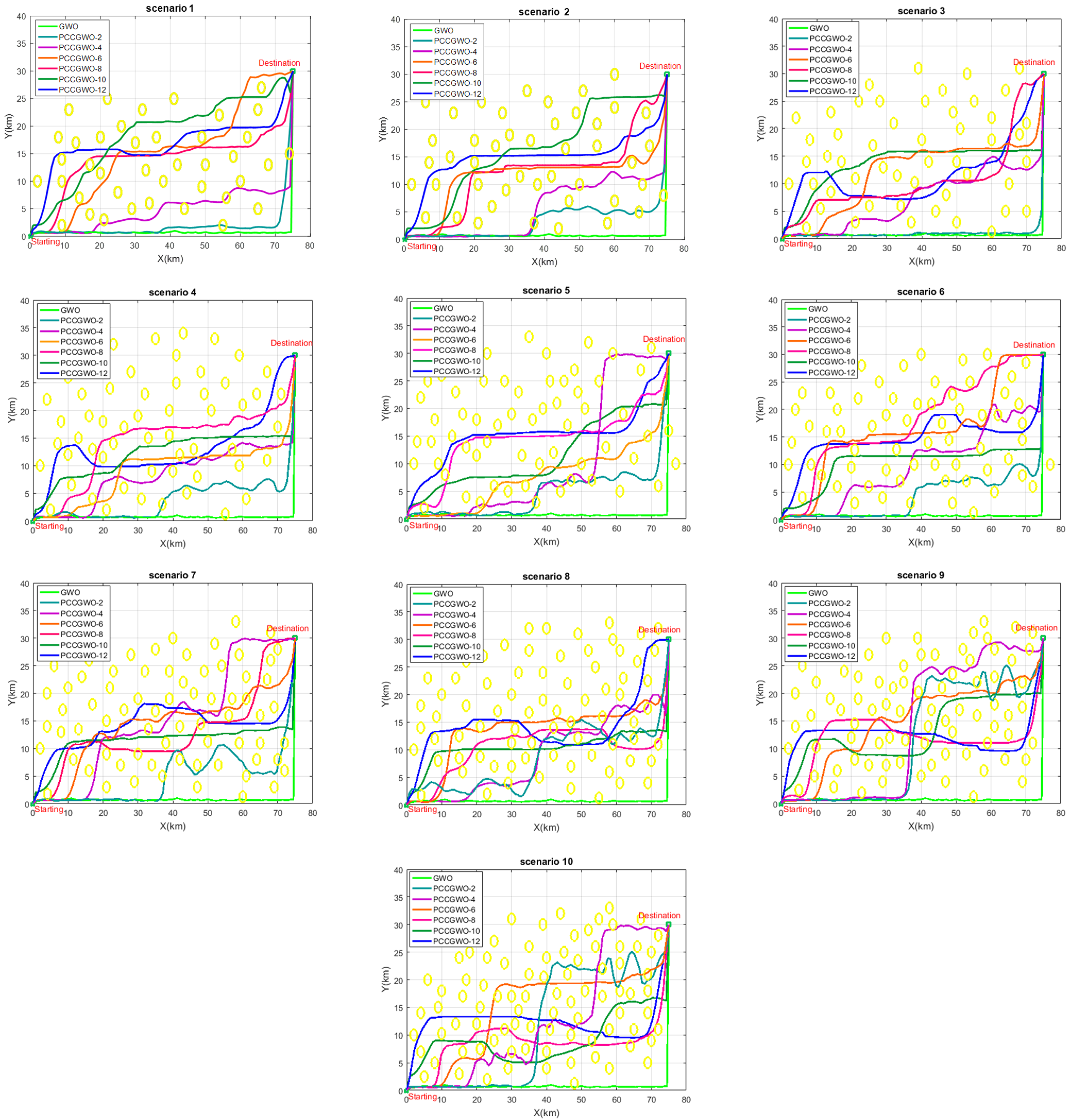
Section 4, demonstrative results over 20 different flight scenarios are carried out and discussed to assess the effectiveness of the proposed planning approach. Section 5 concludes this paper.

2. Path Planning Problem Formulation

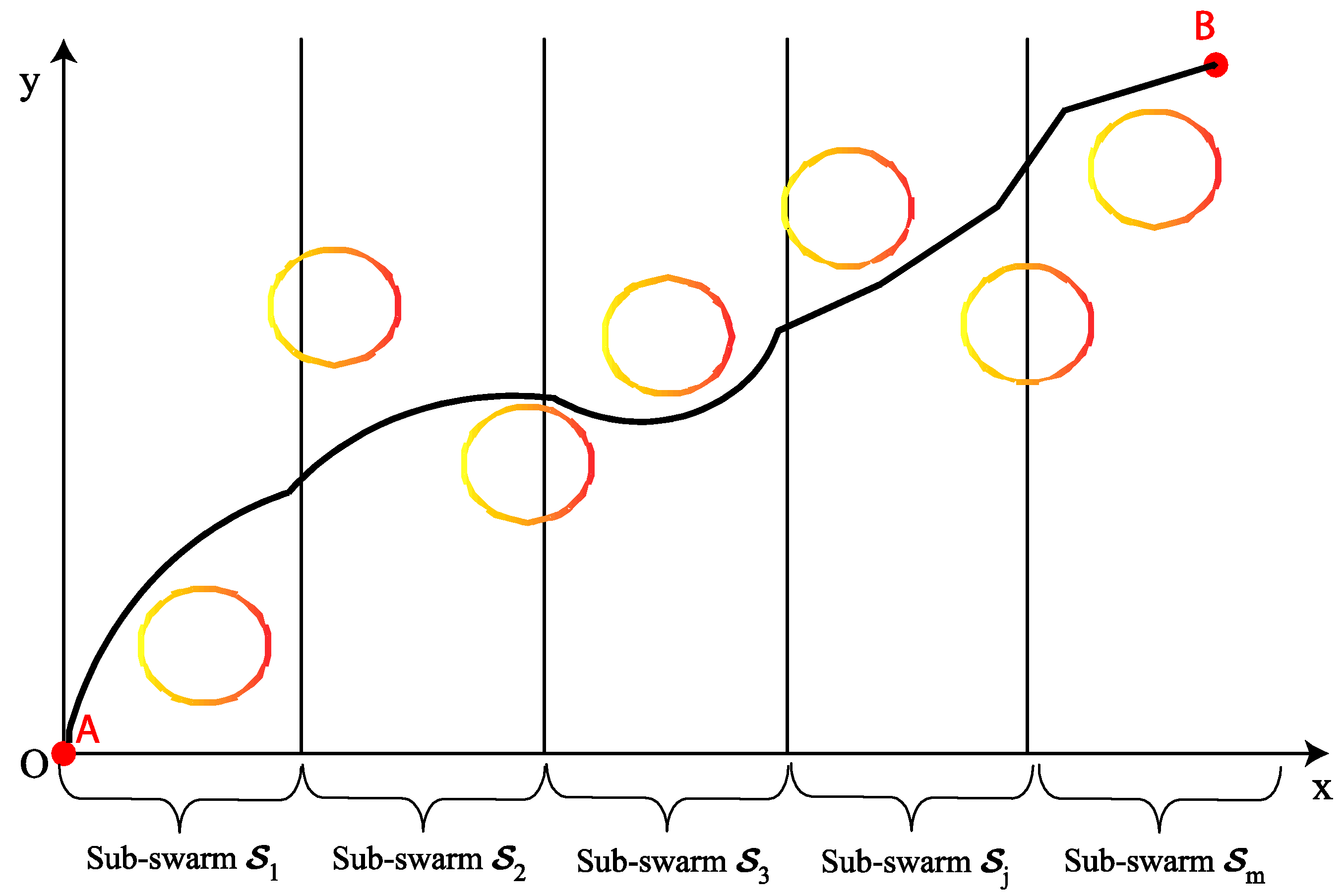
The planning of a flyable and feasible path is a key task in the formalism of drones’ control and navigation. The general definition of such a problem is the generation of a path that guides the drone from a starting point A : ( x 1 , y 1 , z 1 ) to a predefined destination B : ( x n , y n , z n ) . To ensure this, an environmental modeling is required [13,14,16,41]. The x-axis range ( x 1 , x n ) is divided into n 1 equal segments delimited by geometric perpendicular hyper-planes passing through the corresponding points { x 1 , x 2 , , x n } . A waypoint w i = ( x i , y i , z i ) will be taken at each perpendicular plane and a sequence of these generated points Ω A B = { A , ( x 2 , y 2 , z 2 ) , , ( x n 1 , y n 1 , z n 1 ) , B } can be formed. The connection of the different waypoints forming such a flight sequence leads to generating the complete flyable path. In this manner, the path planning problem can be reformulated as an optimization problem that consists in determining the optimal flight waypoints’ sequences minimizing a previously defined performance criterion, i.e., shorter, collision-free and smoother flyable paths [14,41]. In this formulation, the decision variables of such a constrained optimization problem are defined as the vector of coordinates of the waypoints X = ( y 2 , y 3 , , y n 1 , z 2 , z 3 , , z n 1 ) 2 n 4 .
For the drones’ navigation, the length of the flyable path is an essential objective. The shorter path can reduce the flight time and extend the battery life which ensures more safety. Therefore, a shorter path remains desirable in all planning problems. To well formulate such a design goal, the corresponding objective function to be minimized is chosen as follows [14,41]:
f ( X ) = k = 1 n 1 ( x k + 1 x k ) 2 + ( y k + 1 y k ) 2 + ( z k + 1 z k ) 2 ( x n x 1 ) 2 + ( y n y 1 ) 2 + ( z n z 1 ) 2
For any path planning problem, the obstacles’ collision avoidance constraint is a key task. Indeed, to ensure that the planned path is safe, the UAV drone must avoid all obstacles. On the other hand, to avoid the risk of being detected by the radars or missiles, a UAV cannot pass through the dangerous regions and/or fly over them [13,14,16,41]. Thus, such an obstacles’ avoidance constraint is modeled by the following expression:
g 1 ( X ) = ( r o b s i + Δ ) ( x u a v x o b s i ) 2 + ( y u a v y o b s i ) 2 0
where r o b s i and ( x o b s i , y o b s i ) are the radius and position of the ith obstacle, respectively; ( x u a v , y u a v , z u a v ) means the coordinate of the UAV drone, and Δ presents the predefined safety distance between the drone and a detected obstacle.
When a UAV performs angle management, it can influence its dynamic characteristics and make its flight operation inefficient. Therefore, the angle between two adjacent segments is introduced to limit the straightness of the path. This performance constraint can be formulated as follows [42]:
g 2 ( X ) = | φ q , q + 1 | φ max 0
where φ q , q + 1 is the angle between the two adjacent qth and (q+1)th segments connecting the waypoints, and φ max is the maximum value of the steering angle.
Finally, the formulated constrained optimization problem for the UAVs’ path planning procedure is defined as follows:
{ Minimize X D d f ( X ) subject   to : g 1 ( X ) 0 g 2 ( X ) 0
where f ( . ) is the cost function of Equation (1), g 1 ( . ) and g 2 ( . ) are the constraints given by Equations (2) and (3), respectively, X 2 n 4 is the vector of decision variables, and D = { X d | X min X X max } is the bounded d-dimensional search space.
To handle the operational constraints (2) and (3) of the optimization problem (4), a static penalty function-based technique is used as follows [41]:
Φ ( X ) = f ( X ) + i = 1 n c o n κ i max { 0 , g i ( X ) } 2
where κ i are the scaling penalty coefficients and n c o n means the number of constraints.

3. Proposed Parallel Cooperative Coevolutionary Algorithm

3.1. Grey Wolf Metaheuristic

The Grey Wolf Optimizer (GWO) is a swarm intelligence-based algorithm that is inspired by the leadership hierarchy and hunting strategy of grey wolves in nature [43]. Three leader wolves named α, β, and δ are considered in the hierarchy of the GWO formalism. The most dominating member among the group is called alpha (α), followed by beta (β) and delta (δ) ones which help to lead the rest of the wolves, considered as omega (ω) members, toward promising areas. The ith wolf is characterized by its position x k i = ( x k , 1 i , x k , 2 i , , x k , d i ) in the d-dimensional search space. The prey’s position is denoted as x k p = ( x k , 1 p , x k , 2 p , , x k , d p ) . The best candidate solutions α, β, and δ are characterized by their positions x k b e s t , 1 , x k b e s t , 2 , and x k b e s t , 3 .
For hunting a prey, the grey wolves follow the following three main steps, i.e., encircling, hunting, and attacking [43]:
Encircling: To mathematically model the strategy of encircling prey by wolves, the following equations have been proposed:
x k + 1 i = x k p Δ k ϑ k
Δ k = | λ k x k p x k i |
ϑ k = 2 υ k U ( 0 , 1 ) υ k
where λ k are random numbers between 2 and 0, υ k are linearly decreased from 2 to 0 over the iterations course, and U ( 0 , 1 ) is a uniformly random number in [0, 1].
Hunting: The best candidate solutions α, β, and δ guide the other ω wolves to find the global solution of the prey by updating their positions as follows:
x k + 1 i = x k b e s t , 1 + x k b e s t , 2 + x k b e s t , 3 3 , i α , β , δ
where x k b e s t , 1 = x k α Δ k α ϑ 1 , k , x k b e s t , 2 = x k β Δ k β ϑ 2 , k , and x k b e s t , 3 = x k δ Δ k δ ϑ 3 , k .
In Equation (9), the coefficient vectors ϑ 1 , k , ϑ 2 , k , and ϑ 3 , k as well as Δ k α , Δ k β , and Δ k δ are computed as follows:
{ ϑ 1 , k = 2 υ 1 , k U ( 0 , 1 ) υ 1 , k ; ϑ 2 , k = 2 υ 2 , k U ( 0 , 1 ) υ 2 , k ; ϑ 3 , k = 2 υ 3 , k U ( 0 , 1 ) υ 3 , k Δ k α = | λ 1 , k x k α x k i | ; Δ k β = | λ 2 , k x k β x k i | ; Δ k δ = | λ 3 , k x k δ x k i |
where υ j , k , j { 1 , 2 , 3 } , are linearly decreased from 2 to 0 over the iterations course and λ j , k are random numbers distributed uniformly between 2 and 0.
Attacking: To mathematically model the prey attack approach, the value υ k is linearly decreased from 2 to 0 during iterations and involves the reduction of the fluctuation range ϑ k which is a random value in the interval [ 2 υ k , 2 υ k ] . When the value | ϑ k | < 1 , the next positions of wolves will be between their current positions and the prey one that may force them to attack. After the attack and at the next iteration, this process is repeated until the termination criterion is verified.
Finally, a pseudo-code of the basic GWO algorithm is presented by Algorithm 1 as given in [16,20,43].
Algorithm 1: GWO pseudo-code.
1.Randomly initialize the grey wolves’ population.
2.Initialize ϑ j , 0 , υ j , 0 , and λ j , 0 i .
3.Calculate the objective values for each search agent and select x 0 α , x 0 β , and x 0 δ .
4.Update the position of the current search agent.
5.Update ϑ j , k , υ j , k , and λ j , k i
6.Calculate the objective values of all search agents by applying Equation (10).
7.Update the positions x k α , x k β , and x k δ .
8.Check the termination criterion and make iterations repeated.

3.2. Cooperative Coevolutionary Concept

In cooperative coevolutionary algorithms, the optimization problem to be solved is divided into sub-components in the search space and each of them is solved independently by a species or a sub-swarm which is managed by a processor. In mono-objective optimization formalism, Potter and De Jong were the first to propose such a model [25]. The decision variables are split into sub-components and each sub-swarm seeks to optimize its component by applying a standard evolutionary algorithm. These sub-swarms share information among themselves during evolution. To assess the quality of its optimization, a species builds a complete solution with the representative of all other species and its dedicated decision subcomponent. This is how they cooperate in evolution. The representative of the sub-swarm can be defined by their current best individual or by a random choice. For a given sub-swarm, the solutions consist of a fixed part and a variable part to be optimized. The cooperative coevolutionary approach consists of three main steps [25]:
i.
Decomposing the problem: The vector of decision variables is decomposed into smaller sub-components which can be handled by certain evolutionary algorithms.
ii.
Optimizing sub-components: Each sub-component will be evolved separately using an evolutionary algorithm until the stopping criteria are met. This means that each sub-component will be optimized by a sub-swarm.
iii.
Co-adapting sub-components: Since sub-components can be interdependent, co-adaptation is necessary to take these interdependencies into account. They share information among themselves during the evolution process.

3.3. Parallel Master-Slave Model

The master-slave model is one of the most popular approaches for parallel computing due to the simple exploitation of the parallelization capabilities of modern computer systems and its simplicity of implementation. In study [44], Bethke is the first to describe a parallel implementation of an evolutionary algorithm. Subsequently, Grefenstette proposed [45] several prototypes of the parallel evolutionary algorithms representing several variations of the master-slave models. A master-slave model implementation generally requires essential knowledge of the corresponding computer system and minor programming effort. In the master-slave model, one of the processors or cores is selected as the master and the others as slaves of such a master core as shown in Figure 1. The master assigns the slaves hard work or heavy computing tasks and then receives the results from them. The different slaves perform their tasks simultaneously and there is no communication requirement between them. The parallel master-slave model allows a significant reduction in the total computing time required by the algorithm. In such a model of m slaves, the simultaneous evaluation of m individuals is possible, which leads to a significant reduction in the total evaluation time of the population. The parallel software implementation will be more meaningful in large-scale optimization problems [33,34,35,36,37,38,39,40].

3.4. Proposed Parallel Cooperative Coevolutionary Grey Wolf Optimizer

The standard GWO algorithm, initially proposed by Mirjalili in 2014, is prone to convergence prematurity. It is also unable to escape local minima in complex multidimensional optimization problems due to its suffering from the “dimensionality curse”. To overcome these challenges, a Cooperative Coevolutionary Grey Wolf Optimizer (CCGWO) is proposed and used to solve the UAVs’ path planning problem formulated as a large-scale optimization one. The original d-dimensional search space is decomposed into m smaller-dimension subspaces D j denoted as follows:
D = D 1 D 2 D m
Each sub-space should be evaluated by a corresponding sub-swarm. Their dimensions are denoted by d 1 , d 2 , , d m which should verify the following condition:
d = j = 1 m d j ,         d j 1 ,       j = 1 , 2 , , m
where d is the dimension of the original optimization problem.
The standard GWO algorithm employs a single d-dimensional swarm, but the CCGWO one uses m sub-swarms denoted as S 1 , S 2 , , S m . Each of them ensures the optimization in the corresponding subspace D j of dimension d j < d . The size of a given sub-swarm S j is denoted as n S j = | S j | .
The research agents’ evaluation in each sub-swarm of the CCGWO algorithm is identical to that in the standard GWO one as described in Section 3.1. However, this can pose a significant problem. The agents cannot be updated with the objective function due to the missing components. To overcome this problem, a shared buffer vector, also called a context vector, is defined and contains the complete solution by combining all representatives of sub-swarms [27]. This vector provides the missing information required for each particle or research agent to update with the objective function. Let us consider c [ j ] the representative of d j -dimensional for sub-swarm S j :
c [ j ] = ( c 1 [ j ] , c 2 [ j ] , , c d j [ j ] )
The d-dimensional buffer vector C is then obtained by concatenating all different representatives as follows:
C = ( c 1 [ 1 ] , , c d 1 [ 1 ] representative   of   S 1 , c 1 [ 2 ] , , c d 2 [ 2 ] representative   of   S 2 , , c 1 [ m ] , , c d m [ m ] representative   of   S m )
The ith research agent of the jth sub-swarm of CCGWO, as given by Equation (15), is evaluated by completing the missing components from the buffer vector C :
x i [ j ] = ( x i , 1 [ j ] , x i , 2 [ j ] , , x i , d j [ j ] ) D j
To achieve this, the components x i [ j ] are replaced in the buffer’s components that correspond to the representative of the jth sub-swarm by keeping the rest unchanged. Hence, the cost value attributed to x i [ j ] is defined as:
f i [ j ] = f ( C i [ j ] )
where C i [ j ] = ( c 1 [ 1 ] , , c d 1 [ 1 ] unchanged , , x i , 1 [ j ] , , x i , d j [ j ] considered   particle , , c 1 [ m ] , , c d m [ m ] unchanged ) with i = 1 , 2 , , n S j .
The representative of each sub-swarm is defined as its best current individual. To parallelize this described cooperative coevolutionary GWO algorithm without changing its co-evolutionary characteristics, a parallel master-slave model is established, resulting in the proposed PCCGWO algorithm as depicted in Figure 2.
With more details, the master processor will be responsible for initializing the population of research agents, then breaking it down into a set of sub-swarms. Each of them will evolve on part of the problem as a sub-component. The master processor also initializes the buffer vector C using randomly selected individuals from each sub-swarm. After that, it sends to each slave a sub-swarm as well as the buffer vector C . Each slave is designed to evolve a sub-swarm that seeks to optimize its component by applying a standard GWO algorithm for a finite number of times. Such a slave sends the best individuals as representatives to the master after the evolution cycle. The master will build a buffer vector C by concatenating the different representatives and sending it to the different slaves for a new cycle. The master always checks the stop condition, if it is reached, this process will stop. Otherwise, it sends the buffer vector C to all the slaves and asks them to continue the evolutionary process. Finally, Algorithm 2 provides the pseudo-code of the proposed PCCGWO algorithm.
Algorithm 2: PCCGWO pseudo-code.
Master process
1.Randomly initialize the grey wolf population.
2.Decompose the population into m sub-swarms denoted as S 1 , S 2 , , S m .
3.Initialize the buffer C using randomly selected individuals from each sub-swarm.
4.Send each sub-swarm to a slave.
5.Cycle = 0
6.While termination criteria = false do
7.  Parallel for  j = 1 : m slaves
8.  Send to slaves the buffer vector C defined in Equation (14).
9.  Waiting for slaves.
10.  Receive all representatives of sub-swarms from slaves.
11.  End Parallel for
12.  Update the buffer vector C .
13.  Cycle = Cycle + 1
14.End While
Slave [j] process
15.While true do
16.  Receive the buffer vector C from Master process.
17.  Execute GWO on sub-swarm S j .
18.  Send the representative of sub-swarm S j to Master process.
19.End While

3.5. PCCGWO for the UAVs’ Path Planning Problem

In the decision variables vector X = ( y 2 , y 3 , , y n 1 , z 2 , z 3 , , z n 1 ) , the partition rate n is shown as an important design parameter. Such an effective parameter can significantly affect the performance of the optimization algorithm PCCGWO. The more the n number increases, the dimension of the optimization problem increases, thus leading to an increase in the search complexity. Indeed, a higher partition rate will lead to greater route accuracy and greater planning problem complexity. The original d-dimensional search space is decomposed into equal m smaller-dimension sub-spaces. In this problem, the global path is divided into m sub-paths and each sub-component represents a part of the path. Each sub-population is associated to generate the corresponding sub-path as shown in Figure 3.
To start optimization with the PCCGWO algorithm, the initial population with the size n p o p is generated as follows:
P o p w o l v e s = [ y 1 , 2 y 1 , 3 y 1 , n 1 y 2 , 2 y 2 , 3 y 2 , n 1 y n p o p , 2 y n p o p , 3 y n p o p , n 1 z 1 , 2 z 1 , 3 z 1 , n 1 z 2 , 2 z 2 , 3 z 2 , n 1 z n p o p , 2 z n p o p , 3 z n p o p , n 1 ]
Such an initial population is decomposed into m sub-swarms S j . Each of them is associated to evaluate the corresponding sub-component as follows:
S 1 = [ y 1 , 2 [ 1 ] y 1 , 3 [ 1 ] y 1 , ( d 1 / 2 ) + 1 [ 1 ] y 2 , 2 [ 1 ] y 2 , 3 [ 1 ] y 2 , ( d 1 / 2 ) + 1 [ 1 ] y n S 1 , 2 [ 1 ] y n S 1 , 3 [ 1 ] y n S 1 , ( d 1 / 2 ) + 1 [ 1 ] z 1 , 2 [ 1 ] z 1 , 3 [ 1 ] z 1 , ( d 1 / 2 ) + 1 [ 1 ] z 2 , 2 [ 1 ] z 2 , 3 [ 1 ] z 2 , ( d 1 / 2 ) + 1 [ 1 ] z n S 1 , 2 [ 1 ] z n S 1 , 3 [ 1 ] z n S 1 , ( d 1 / 2 ) + 1 [ 1 ] ]                 S j = [ y 1 , ( i = 1 j 1 ( d i / 2 ) ) + 2 [ j ] y 1 , ( i = 1 j 1 ( d i / 2 ) ) + 3 [ j ] y 1 , ( i = 1 j ( d i / 2 ) ) + 1 [ j ] y 2 , ( i = 1 j 1 ( d i / 2 ) ) + 2 [ j ] y 2 , ( i = 1 j 1 ( d i / 2 ) ) + 3 [ j ] y 2 , ( i = 1 j ( d i / 2 ) ) + 1 [ j ] y n S j , ( i = 1 j 1 ( d i / 2 ) ) + 2 [ j ] y n S j , ( i = 1 j 1 ( d i / 2 ) ) + 3 [ j ] y n S j , ( i = 1 j ( d i / 2 ) ) + 1 [ j ] z 1 , ( i = 1 j 1 ( d i / 2 ) ) + 2 [ j ] z 1 , ( i = 1 j 1 ( d i / 2 ) ) + 3 [ j ] z 1 , ( i = 1 j ( d i / 2 ) ) + 1 [ j ] z 2 , ( i = 1 j 1 ( d i / 2 ) ) + 2 [ j ] z 2 , ( i = 1 j 1 ( d i / 2 ) ) + 3 [ j ] z 2 , ( i = 1 j ( d i / 2 ) ) + 1 [ j ] z n S j , ( i = 1 j 1 ( d i / 2 ) ) + 2 [ j ] z n S j , ( i = 1 j 1 ( d i / 2 ) ) + 3 [ j ] z n S j , ( i = 1 j ( d i / 2 ) ) + 1 [ j ] ]                 S m = [ y 1 , ( i = 1 K 1 ( d i / 2 ) ) + 2 [ m ] y 1 , ( i = 1 m 1 ( d i / 2 ) ) + 3 [ m ] y 1 , n 1 [ m ] y 2 , ( i = 1 K 1 ( d i / 2 ) ) + 2 [ m ] y 2 , ( i = 1 m 1 ( d i / 2 ) ) + 3 [ m ] y 2 , n 1 [ m ] y n S m , ( i = 1 m 1 ( d i / 2 ) ) + 2 [ m ] y n S m , ( i = 1 m 1 ( d i / 2 ) ) + 3 [ m ] y n S m , n 1 [ m ] z 1 , ( i = 1 m 1 ( d i / 2 ) ) + 2 [ m ] z 1 , ( i = 1 m 1 ( d i / 2 ) ) + 3 [ m ] z 1 , n 1 [ m ] z 2 , ( i = 1 m 1 ( d i / 2 ) ) + 2 [ m ] z 2 , ( i = 1 m 1 ( d i / 2 ) ) + 3 [ m ] z 2 , n 1 [ m ] z n S m , ( i = 1 m 1 ( d i / 2 ) ) + 2 [ m ] z n S m , ( i = 1 m 1 ( d i / 2 ) ) + 3 [ m ] z n S m , n 1 [ m ] ]
with d = j = 1 m d j and n p o p = j = 1 m n S j .

4. Results and Discussion

4.1. Parallel Computing Environment

To pass from a sequential program to a parallel one, the parallelization process is the most efficient attempt. Parallel computing is a powerful way to speed up conception time and the prototyping process. The implementation of a parallel algorithm is highly dependent on the hardware architecture on which the program will be run, but it is also influenced by the software environment. In this work, the MIMD (Multiple Instruction, Multiple Data) systems are used as shared memory architectures commonly known as the multiprocessor. Such hardware/software architecture corresponds to sets of interconnected processors that share the same memory space. Today, most computers have multiple processors, i.e., containing one or more cores, and therefore fall into the family of multiprocessor systems. In a shared memory system, different cores can run in parallel within a process. Threads have access to the common global memory but have their execution stack. The “Parallel Computing Toolbox” software of MATLAB environment allows doing multithreaded programming [46]. In this work, the simplest “Parfor” structure in the MATLAB tool is used to illustrate this functionality. The workers’ number is equal to the iterations number of the parallel loop. MATLAB workers perform iterations independently of each other. They evolve in parallel in the proposed PCCGWO algorithm (one per sub-population). By using Parfor, workers are anonymous, have their execution stack, and share common global memory.

4.2. Numerical Experimentations

To illustrate the performance of the proposed PCCGWO algorithm to solve the formulated UAVs’ path planning problem, numerical experimentations with six versions of PCCGWO are carried out and discussed. These proposed PCCGWO versions implement algorithms with different sub-populations equal to 2, 4, 6, 8, 10, and 12. These parallel cooperative coevolutionary algorithms with different sub-swarms are denoted as PCCGWO-2, PCCGWO-4, PCCGWO-6, PCCGWO-8, PCCGWO-10, and PCCGWO-12. In this work, the performances of the proposed PCCGWO algorithms in terms of solution quality and computational speedup are compared to those of the standard GWO one. The effectiveness of the proposed versions of PCCGWO in solving the path planning problem is presented and analyzed under 20 different flight scenarios as described in Table 1.
To assess the effectiveness of the proposed planning approach, these 20 scenarios are different from each other in terms of the number and position of the obstacles as well as the dimension of the planning problem. The problem dimension and obstacles’ number are increased over the scenarios to increase the complexity and hardness of the flight mission. To have equitable and reliable comparisons, the common parameters of the proposed PCCGWO algorithms such as the population size and the maximum number of iterations are set as n p o p = 1200 and n i t e r = 1500 , respectively. The proposed parallel cooperative coevolutionary algorithms are coded under the MATLAB 2016a environment, and executed on a computer with a Core i5 processor, having 12 cores at 2.90 GHz and 8.00 GB of RAM.

4.2.1. Solution Quality’s Analysis

The proposed parallel cooperative coevolutionary algorithms are performed on the formulated path planning problem given by Equation (4). The six versions of PCCGWO are, however, compared with the standard version of the GWO metaheuristic for the considered different flight scenarios. Three performance criteria such as the value of standardized costs, the path length, and the threats’ avoidance capability are used in each scenario to assess the solution quality. All the proposed GWO and PCCGWO algorithms are executed 20 times independently in each scenario in Table 1. The statistical results of the numerical experimentations under 20 independent runs are summarized in Table 2. All the proposed algorithms are compared based on the objective function value obtained in the best, worst, and mean optimization cases. A smaller standard deviation (STD) value indicates better reproducibility of the optimization algorithm across independent optimization tests. On the other hand, the threats’ avoidance capability of the reported algorithms is quantified by the computation of the PF (Path’s Feasibility) metric. Such a performance index means the percentage of the feasible paths satisfying the operational constraints of the planning problem, i.e., non-collision flight.
While considering the length of the flyable path as an optimization criterion of the problem (4), the investigated Straight-Line Rate (SLR) index is defined as follows:
S L R = p a t h length / | A B |
where | A B | is the straight line’s length between starting point A and destination B.
A smaller value of the SLR index indicates a better efficiency of the used planning algorithm. The statistical results of numerical experiments over the considered 20 flight instances and under 20 independent runs are summarized in Table 3. All versions of the proposed PCCGWO algorithm are compared to the standard GWO.
From the statistical results of Table 2 and Table 3, one can observe that the best mean cost values and SLR performance indexes are often obtained with the variants of the algorithm with the highest number of slaves, i.e., PCCGWO-10 and PCCGWO-12 ones. Indeed, for this large planning benchmark with 20 instances, as the dimension of the planning problem and the number of obstacles increase, the PF metric decreases for most variants of the PCCGWO algorithms, except those having more increased slaves in their parallel computation mechanisms. Finding a feasible path becomes more difficult when the number of slaves is reduced for instances with high numbers of obstacles and problem dimensions. The proposed PCCGWO-12 algorithm with 12 slaves becomes, on average, the best performing algorithm with tighter forms of the SLR data distribution over the different instances, followed by the PCCGWO-10 and PCCGWO-8 ones.
On the other hand, Figure 4 shows the Box-and-Whisker plots for the proposed parallel cooperative coevolutionary algorithms over the 20 flight scenarios. In Figure 4, the x-axes of different curves denote the reported algorithms’ names, i.e., 1: GWO, 2: PCCGWO-2, 3: PCCGWO-4, and so on, as shown in the figure’s legend. From these demonstrative results, one can observe that the algorithms with an increased number of slaves, i.e., PCCGWO-10 and PCCGWO-12 variants, often give tighter forms of the SLR data distribution.
On the other hand, and for the threats’ avoidance criterion, some illustrations of the planned paths corresponding to the average case of performance are shown in Figure 5, Figure 6, Figure 7 and Figure 8 for the flight scenarios 5, 9, 17, and 20 of Table 1, respectively. As shown in Figure 5, Figure 6, Figure 7 and Figure 8, all versions of the proposed PCCGWO algorithm are more efficient than the standard GWO in terms of the solution’s quality and fastness convergence. The exploration and exploitation capacities of PCCGWO algorithms are further improved. In scenarios 5 and 9, with problem dimensions equal to 200 and 300, respectively, all versions of the PCCGWO algorithms as well as the standard GWO one give feasible paths and can avoid all obstacles. In scenario 17, with problem dimensions equal to 500, only the PCCGWO-6, PCCGWO-8, PCCGWO-10, and PCCGWO-12 optimizers avoid the danger zones. In scenario 20, with a problem dimension equal to 600 and a high number of obstacles, only the proposed PCCGWO-10 and PCCGWO-12 algorithms give feasible paths. It is obvious that for an increase in the problem dimension, some PCCGWO algorithms become inefficient, due to the fewer number of slaves which become insufficient to provide efficient parallel computing and good research cooperation. In this case, variants of PCCGWO with a higher number of slaves are needed and more sophisticated processors with more than 12 cores are then necessary for these treatments. Additionally, one can observe that the standard GWO never moves between obstacles in the considered flight scenarios. On the contrary, all versions of PCCGWO pass between obstacles to reach the target point. The PCCGWO algorithm remains the more suited solver for performing flight missions with high efficiency compared to the GWO one.
Let us now analyze the effect of slaves’ number, for a given problem dimension, on the performance of the proposed PCCGWO-based planning process. For this purpose, another 10 flight scenarios, for the same dimension equal to 600 and various numbers and positions of obstacles, are investigated as shown in Table 4. From this result, one can observe that the increase in the number of slaves leads to a decrease in the SLR values. For the threats’ avoidance, the planned paths are shown in Figure 9. In scenarios 1, 2, and 3 of Table 4, with fewer numbers of obstacles, the algorithms PCCGWO-6, PCCGWO-8, PCCGWO-10, and PCCGWO-12 avoid the danger zones. In scenario 4, only the algorithms PCCGWO-8, PCCGWO-10, and PCCGWO-12 give feasible paths. For more complex scenarios, i.e., flight environment with several obstacles, only the PCCGWO-10 and PCCGWO-12 variants give feasible collision-free paths. Thus, for a concrete number of problem dimensions, as the number of obstacles increases, more slaves in the PCCGWO algorithm are needed to find feasible paths. The shorter and collision-free obtained paths confirm the superiority and effectiveness of the proposed PCCGWO optimizers with an increased number of slaves, i.e., PCCGWO-10 and PCCGWO-12 variants. Obviously, with each increase in the dimension of the planning problem, algorithms with more slaves are needed to best handle the complexity of the resulting optimization problem.
Considering the two performance criteria, i.e., standardized cost and SLR, a statistical comparison based on the nonparametric Friedman test is implemented and discussed according to the mean values of performance over 20 different instances. The aim is to statistically study significant differences between the considered PCCGWO variants and standard GWO. For the seven reported algorithms ( ζ = 7 ) and the twenty scenarios ( η = 20 ), the Iman–Davenport extension of the classical Friedman test [47] leads to the computed value F F 1 = 52 . 7465 for the objective value criterion and F F 2 = 71 . 2460 for the SLR criterion. Based on the F distribution table, the critical value with ζ 1 and ( ζ 1 ) ( η 1 ) degree-of-freedom is equal to F 6 , 114 , 0.05 = 2.1750 < F F 1 < F F 2 at a confidence level of α = 0.05 . The null hypothesis is therefore rejected and there are significant differences between the performances of the proposed algorithms in solving the path planning problem. Fisher’s LSD post hoc test [48] is applied to find out which algorithms differ from others. The ranks’ sums for all proposed algorithms are summarized in Table 5 and Table 6. When the absolute difference of the ranks’ sum of two algorithms is greater than a critical value, they are declared to be different. Based on the statistical calculation formula given in [48], the critical value is equal to 11.9624 for the standardized cost criterion and 10.6661 for the SLR criterion. Paired comparisons are summarized in Table 7 and Table 8. The underlined values indicate the difference in the performance of the proposed algorithms. From the conducted statistical study, one can see that the standard GWO is the worst performing algorithm according to the standardized cost and SLR criteria of the UAVs’ path planning problem. The six PCCGWO versions surpass the standard GWO in all scenarios with statistical confidence. Indeed, the proposed algorithm PCCGWO-12 becomes the best, followed by PCCGWO-10 and PCCGWO-8 ones. The total number of subpopulations has a big impact on the performance of the PCCGWO algorithms. These demonstrative results show that the proposed PCCGWO algorithm improves the quality of the standard GWO-based solutions.

4.2.2. Computational Time

The performance of the proposed PCCGWO algorithms can be analyzed and compared in terms of the runtime of all reported algorithms over 20 different flight scenarios. The statistical results obtained for the Computational (CT) metric are summarized in Table 9. The obtained runtime measures for the mean case of optimization are also graphically shown in Figure 10. From these demonstrative results, one can notice that the increase in the number of slaves in the parallel master-slave model leads to lower runtimes of the reported PCCGWO algorithms. The PCCGWO-10 and PCCGWO-12 with the highest number of slaves are often the best variants with a remarkable superiority regarding the other reported PCCGWO algorithms. The reason for these fast processing computations is that the population and the decision variables are divided by the number of slaves that are evolved in parallel, i.e., one per subpopulation. It is also noticed that as the size of the problem increases, the runtime increases for all PCCGWO versions. As expected, a heavier computational and communication burden in parallel algorithms may be imposed by the manipulation and transmission of higher dimensional vectors.

4.2.3. Algorithms’ Sensitivity Analysis

In this subsection, a study on the impact of the main control parameters’ settings of the PCCGWO versions, i.e., population size n p o p and maximum number of iterations n i t e r , is carried out while considering the path length and the execution time as performance metrics. For this sensitivity analysis of the proposed PCCGWO algorithms, several simulations with different settings of control parameters, as n p o p { 1200 , 1600 , 2000 } , and n i t e r { 1500 , 2000 , 2500 } , are performed and summarized in Table 10 and Table 11 for the considered two performance metrics. For a given numerical experimentation, the impact of a single parameter is examined while keeping the other parameter constant. All the performance comparisons are conducted under Scenario 20 of Table 1 which represents the hardest and most complicated path planning instance.
From these demonstrative results, one can notice that the increase in the population size leads to a decrease in the path length and, subsequently, an increase in the execution time for all reported algorithms. It is also obvious that the elapsed time increases linearly with the increase in the number of iterations, on the contrary, the path length decreases. In Scenario 20 of Table 1, the PCCGWO-6, PCCGWO-8, PCCGWO-10, and PCCGWO-12 algorithms give achievable paths while avoiding all the obstacles. With parameters’ setting n p o p = 1200 and n i t e r = 1500 , only the PCCGWO-10 and PCCGWO-12 algorithms give feasible paths while respecting the collision avoidance constraint. Therefore, as the size population and number of iterations increase, the efficiency of the proposed PCCGWO metaheuristics algorithms improves.

4.2.4. Comparison with Other Metaheuristics Algorithms

To examine and evaluate the performance of the proposed PCCGWO-12, recent and extensively used Water Cycle Algorithm (WCA), Crow Search Algorithm (CSA), Salp Swarm Algorithm (SSA), and Multi-Verse Optimizer (MVO) are considered for the comparison. For these algorithms, the common parameters such as the population size and the maximum number of iterations are set as n p o p = 1200 and n i t e r = 1500 , respectively. All the performance comparisons are conducted under Scenario 20 of Table 1. All the compared algorithms are independently executed 20 times. The specific control parameters of each reported metaheuristic are summarized as follows:
WCA [49]: number of rivers: 4, maximum distance: 1 × 10⁻¹⁶.
SSA [50]: no control parameters.
CSA [51]: awareness probability: 0.2, flight length: 1.
MVO [52]: min and max of wormhole existence probabilities: 0.2 and 1.
Table 12 presents the optimization results of the compared algorithms in terms of SRL and CT performance criteria. Based on these results, one can observe the superiority of the proposed PCCGWO-12 algorithm in terms of solutions’ quality, results’ reproducibility, and computational speedup, i.e., lower values for the mean SLR criterion, STD indices, and computational time.
Figure 11 shows the planned paths of the proposed and compared algorithms. Shorter and collision-free paths are obtained by the PCCGWO-12 planner that also better performs the fastest computation processing. On the contrary, all other reported algorithms are not efficient enough for the considered planning problem with increased numbers of obstacles and dimensions. Some of these planners lead to not flyable paths that traverse the threat zones with a lot of fluctuations. This weakness of WCA, SSA, CSA, and MVO algorithms in the planning process is due to their “dimensionality curse” that often makes failure to solve such large-scale optimization problems. In addition, the exploration and exploitation capacities of the proposed PCCGWO-12 algorithm are superior compared to those of the reported WCA, SSA, CSA, and MVO algorithms. Based on these established comparisons and observations, the superiority and effectiveness of the proposed PCCGWO-based path planning approach are further improved in terms of collision avoidance, shorter planned paths, and fastness of the computation processing. The novelty and originality of our work are well clarified compared to approaches using similar techniques.

5. Conclusions

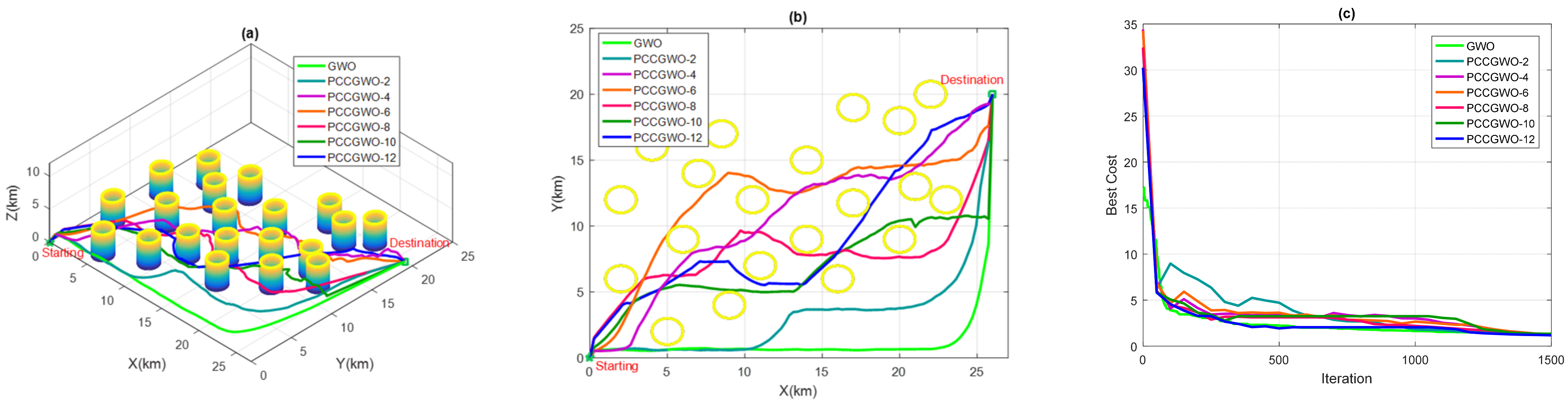
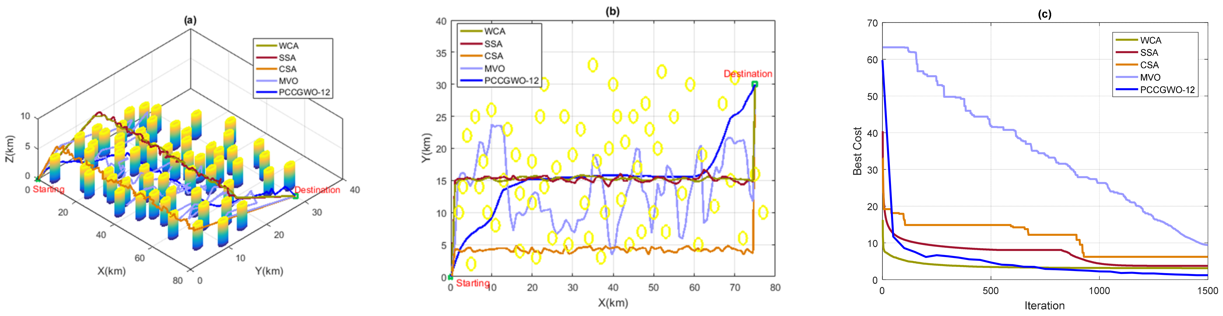
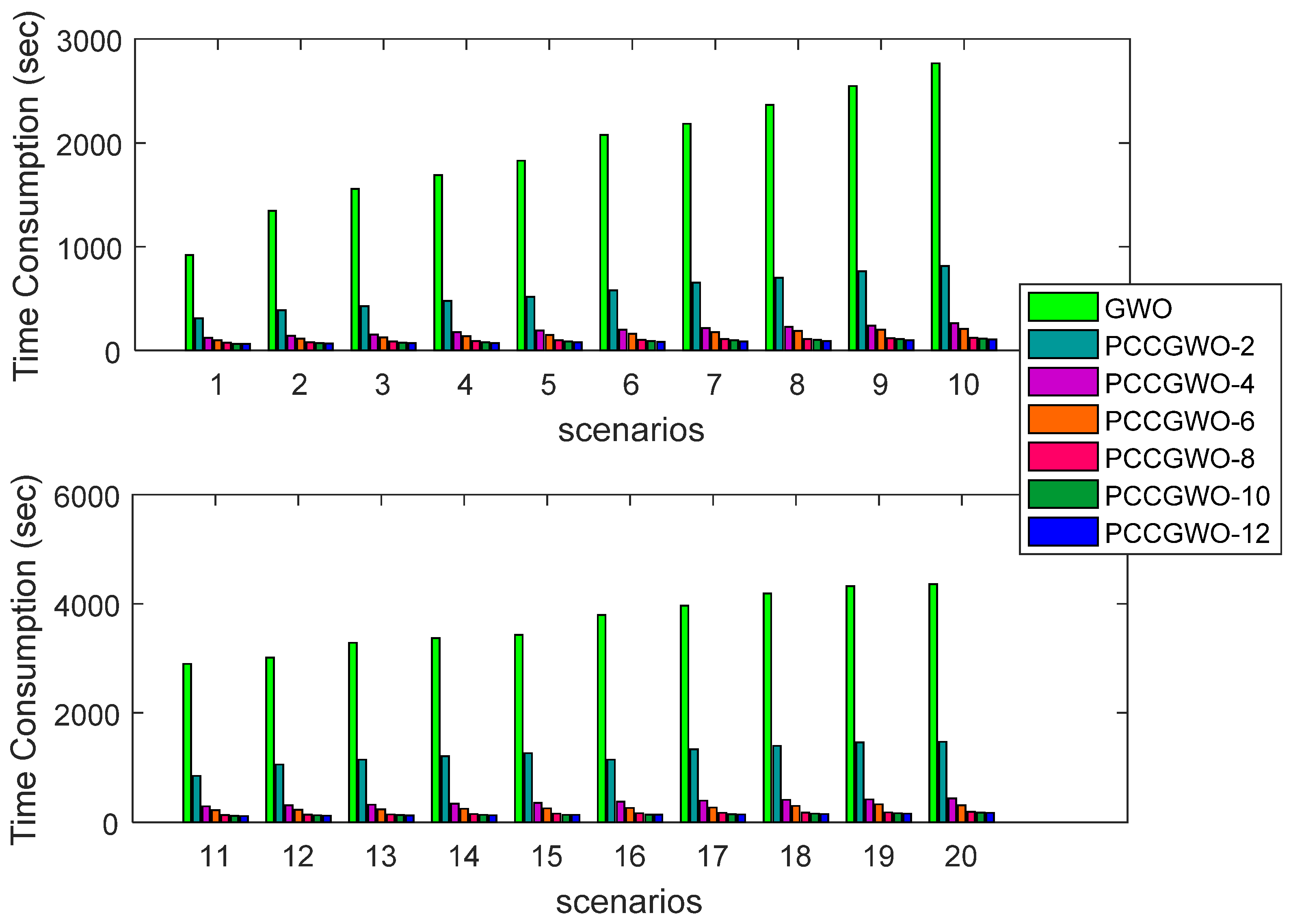
In this paper, a new Parallel Cooperative Coevolutionary variant of the Grey Wolf Optimizer (PCCGWO) based on a parallelization master-slave model has been proposed and successfully applied to solve the UAVs’ path planning problem over large benchmarks and instances of navigation. To overcome the limits and drawbacks of the standard GWO for solving large-scale and complex path planning problems, particularly in terms of dimensionality curse and prohibitive time consuming, two improvement mechanisms in terms of parallelization and cooperative co-evolutionary search are introduced in the proposed PCCGWO algorithm. The UAVs’ path planning problem is formulated as an LSGO problem under operational constraints mainly in terms of obstacles’ collision avoidance and path’s straightness. A cooperative coevolutionary mechanism is applied to make an efficient partition of the original search space into smaller dimensional sub-spaces. The decision variables’ vector is decomposed into several subcomponents with reduced dimensions. An efficient parallelization master-slave technique is then proposed to further reduce the computation time faced with the large-scale and hardness of the planning problem. Six PCCGWO variants with an increased number of slaves, i.e., PCCGWO-2, PCCGWO-4, PCCGWO-6, PCCGWO-8, PCCGWO-10, and PCCGWO-12, are proposed according to the number of the partitioned sub-populations and the available cores of the computer CPU’s processor. Each slave of such a parallel architecture is designed to evolve a sub-swarm that seeks to optimize its component by applying a standard GWO algorithm. The master builds a buffer vector by concatenating the different representatives from slaves, shown as best search agents, and sending it again for a new cycle. The performance analysis of the proposed PCCGWO planners is carried out based on several experiments over different flight instances as well as a comparative study with the standard GWO algorithm, and other recent and extensively used metaheuristics, i.e., Water Cycle Algorithm (WCA), Crow Search Algorithm (CSA), Salp Swarm Algorithm (SSA), and Multi-Verse Optimizer (MVO). The demonstrative results, as well as the nonparametric statistical analyses in the sense of Friedman and post hoc tests, show the effectiveness and superiority of the proposed PCCGWO algorithms with the highest number of slaves, i.e., PCCGWO-10 and PCCGWO-12 variants. The performance metrics in terms of shorter and collision-free planned paths and computational speedup are significantly improved. Obviously, with each increase in the planning problem dimension and number of obstacles, i.e., a more intensive partition of the flight environment, PCCGWO variants with more slaves are needed to best handle the complexity of the resulting optimization problem. As the most suitable drone planners are the ones that have the least parameters’ tuning with an increased computation speediness regarding the software/hardware specifications of the onboard control units, the proposed PCCGWO algorithm can be considered as a promising method for providing shorter and collision-free flight paths in real-world environments.
Future works deal with the implementation of the proposed PCCGWO-based path planning method using the real-world Parrot AR. Drone 2.0 prototype of UAVs and the associated MATLAB/Simulink software. The real-world implementation and prototyping of such a planning algorithm will be investigated regarding all engineering details and managerial implications.

Author Contributions

Conceptualization, R.J. and S.B.; methodology, S.B.; software, R.J.; validation, M.A.-D., H.R. and S.B.; formal analysis, H.R.; investigation, R.J.; resources, S.B.; data curation, M.A.-D.; writing—original draft preparation, R.J.; writing—review and editing, S.B.; visualization, M.A.-D.; supervision, S.B.; project administration, H.R.; funding acquisition, H.R. and M.A.-D. All authors have read and agreed to the published version of the manuscript.

Funding

This research received no external funding.

Informed Consent Statement

Not applicable.

Data Availability Statement

No new data were created or analyzed in this study.

Acknowledgments

The authors acknowledge the support of King Fahd University of Petroleum & Minerals, Saudi Arabia.

Conflicts of Interest

The authors declare no conflict of interest.

References

  1. Mukhamediev, R.I.; Symagulov, A.; Kuchin, Y.; Zaitseva, E.; Bekbotayeva, A.; Yakunin, K.; Assanov, I.; Levashenko, V.; Popova, Y.; Akzhalova, A.; et al. Review of Some Applications of Unmanned Aerial Vehicles Technology in the Resource-Rich Country. Appl. Sci. 2021, 11, 10171. [Google Scholar] [CrossRef]
  2. Rodríguez, M.V.; Melgar, S.G.; Cordero, A.S.; Márquez, J.M.A. A Critical Review of Unmanned Aerial Vehicles (UAVs) Use in Architecture and Urbanism: Scientometric and Bibliometric Analysis. Appl. Sci. 2021, 11, 9966. [Google Scholar] [CrossRef]
  3. Khelifi, A.; Ciccone, G.; Altaweel, M.; Basmaji, T.; Ghazal, M. Autonomous Service Drones for Multimodal Detection and Monitoring of Archaeological Sites. Appl. Sci. 2021, 11, 10424. [Google Scholar] [CrossRef]
  4. Lopez, R.L.; Sanchez, M.J.B.; Jimenez, M.P.; Arrue, B.C.; Ollero, A. Autonomous UAV System for Cleaning Insulators in Power Line Inspection and Maintenance. Sensors 2021, 21, 8488. [Google Scholar] [CrossRef]
  5. Gao, X.; Hou, Z.; Zhu, X.F.; Zhang, J.T.; Chen, X.Q. The shortest path planning for manoeuvres of UAV. Acta Polytech. Hungarica 2013, 10, 221–239. [Google Scholar]
  6. Zhang, J.; Li, J.; Yang, H.; Feng, X.; Sun, G. Complex Environment Path Planning for Unmanned Aerial Vehicles. Sensors 2021, 21, 5250. [Google Scholar] [CrossRef]
  7. Lee, W.; Jeon, Y.; Kim, T.; Kim, Y.-I. Deep Reinforcement Learning for UAV Trajectory Design Considering Mobile Ground Users. Sensors 2021, 21, 8239. [Google Scholar] [CrossRef] [PubMed]
  8. Qayyum, T.; Trabelsi, Z.; Malik, A.; Hayawi, K. Trajectory Design for UAV-Based Data Collection Using Clustering Model in Smart Farming. Sensors 2022, 22, 37. [Google Scholar] [CrossRef]
  9. Huang, C.; Fei, J. UAV Path Planning Based on Particle Swarm Optimization with Global Best Path Competition. Int. J. Pattern Recognit. Artif. Intell. 2018, 32. [Google Scholar] [CrossRef]
  10. Jamshidi, V.; Nekoukar, V.; Refan, M.H. Analysis of parallel genetic algorithm and parallel particle swarm optimization algorithm UAV path planning on controller area network. Int. J. Control Autom. Syst. 2019, 31, 129–140. [Google Scholar] [CrossRef]
  11. Tuba, E.; Dolicanin, E.; Tuba, M. Water Cycle Algorithm for Robot Path Planning. In Proceedings of the 2018 10th International Conference on Electronics, Computers and Artificial Intelligence, Iasi, Romania, 28–30 June 2018. [Google Scholar]
  12. Shao, S.; Peng, Y.; He, C.; Du, Y. Efficient path planning for UAV formation via comprehensively improved particle swarm optimization. ISA Trans. 2020, 97, 415–430. [Google Scholar] [CrossRef]
  13. Jarray, R.; Bouallègue, S. Intelligent Decision Making Approach for Multi-Criteria Path Planning of Unmanned Aerial Vehicles. In Proceedings of the 7th International Conference on Automation, Control Engineering & Computer Science, Sousse, Tunisia, 12–13 October 2020. [Google Scholar]
  14. Jarray, R.; Bouallegue, S. Multi-Verse Algorithm based Approach for Multi-criteria Path Planning of Unmanned Aerial Vehicles. Int. J. Adv. Comput. Sci. Appl. 2020, 11. [Google Scholar] [CrossRef]
  15. Soundarya, M.S.; Anusha, D.K.; Rohith, P.; Panneerselvam, K.; Srinivasan, S. Optimal path planning of UAV using grey wolf optimizer. Int. J. Comput. Sci. Eng. 2019, 5, 129–136. [Google Scholar]
  16. Jarray, R.; Bouallègue, S. Paths Planning of Unmanned Aerial Vehicles based on Grey Wolf Optimizer. In Proceedings of the 4th International Conference on Advanced Systems and Emergent Technologies, Hammamet, Tunisia, 17–20 March 2020. [Google Scholar]
  17. Zhang, W.; Zhang, S.; Wu, F.; Wang, Y. Path Planning of UAV Based on Improved Adaptive Grey Wolf Optimization Algorithm. IEEE Access 2021, 9, 89400–89411. [Google Scholar] [CrossRef]
  18. Yang, L.; Guo, J.; Liu, Y. Three-dimensional UAV cooperative path planning based on the MP-CGWO algorithm. International Int. J. Innov. Comput. Inf. Control 2020, 16, 991–1006. [Google Scholar]
  19. Kumar, R.; Singh, L.; Tiwari, R. Path planning for the autonomous robots using modified grey wolf optimization approach. J. Intell. Fuzzy Syst. 2021, 40, 9453–9470. [Google Scholar] [CrossRef]
  20. Fessi, R.; Rezk, H.; Bouallègue, S. Grey wolf optimization based tuning of terminal sliding mode controllers for a quadrotor. Comput. Mater. Contin. 2021, 68, 2256–2282. [Google Scholar] [CrossRef]
  21. Nadimi-Shahraki, M.H.; Taghian, S.; Mirjalili, S. An improved grey wolf optimizer for solving engineering problems. Expert Syst. Appl. 2021, 166, 113917. [Google Scholar] [CrossRef]
  22. Ahmadi, R.; Ekbatanifard, G.; Bayat, P. A Modified Grey Wolf Optimizer Based Data Clustering Algorithm. Appl. Artif. Intell. 2020, 35, 63–79. [Google Scholar] [CrossRef]
  23. Lu, C.; Gao, L.; Li, X.; Hu, C.; Yan, X.; Gong, W. Chaotic-based grey wolf optimizer for numerical and engineering optimization problems. Memetic Comput. 2020, 12, 371–398. [Google Scholar] [CrossRef]
  24. Liu, Y.; Lu, H. A Strategy of Multi-UAV Cooperative Path Planning Based on CCPSO. In Proceedings of the 2019 IEEE International Conference on Unmanned Systems, Beijing, China, 17–19 October 2019. [Google Scholar]
  25. Potter, M.A.; De Jong, K.A. A Cooperative Coevolutionary Approach to Function Optimization. In Proceedings of the 3rd Parallel Problem Solving from Nature—PPSN III, Jerusalem, Israel, 9–14 October 1994. [Google Scholar]
  26. Sarkar, R.; Barman, D.; Chowdhury, N.A. Cooperative Co-evolutionary Genetic Algorithm for Multi-Robot Path Planning Having Multiple Targets. In Computational Intelligence in Pattern Recognition; Das, A., Nayak, J., Naik, B., Pati, S., Pelusi, D., Eds.; Springer: Singapore, 2020; Volume 999, pp. 727–740. [Google Scholar]
  27. Bergh, F.V.D.; Engelbrecht, A. A Cooperative Approach to Particle Swarm Optimization. IEEE Trans. Evol. Comput. 2004, 8, 225–239. [Google Scholar] [CrossRef]
  28. Sanchez-Ante, G.; Ramos, F.; Frausto, J. Cooperative Simulated Annealing for Path Planning in Multi-Robot Systems. In Proceedings of the Mexican International Conference on Artificial Intelligence, Acapulco, Mexico, 11–14 April 2000. [Google Scholar]
  29. Doerner, K.F.; Hartl, R.F.; Reimann, M. Cooperative Ant Colonies for Optimizing Resource Allocation in Transportation. In Applications of Evolutionary Computing; Boers, E.J.W., Ed.; Springer: Berlin/Heidelberg, Germany, 2001; Volume 2037, pp. 70–79. [Google Scholar]
  30. Yang, Z.; Tang, K.; Yao, X. Large scale evolutionary optimization using cooperative coevolution. Inf. Sci. 2008, 178, 2985–2999. [Google Scholar] [CrossRef] [Green Version]
  31. Vakhnin, A.; Sopov, E. Improving DE-Based Cooperative Coevolution for Constrained Large-Scale Global Optimization Problems Using an Increasing Grouping Strategy. In Proceedings of the II International Scientific Conference on Advanced Advanced Technologies in Aerospace, Mechanical and Automation Engineering- MIST: Aerospace, Krasnoyarsk, Russia, 18–21 September 2019. [Google Scholar]
  32. Trunfio, G.A. Enhancing the firefly algorithm through a cooperative coevolutionary approach: An empirical study on benchmark optimization problems. Int. J. Bio-Inspir. Com. 2014, 6, 108–125. [Google Scholar] [CrossRef]
  33. Zhou, Y.; He, F.; Hou, N.; Qiu, Y. Parallel ant colony optimization on multi-core SIMD CPUs. Future Gener. Comput. Syst. 2018, 79, 473–487. [Google Scholar] [CrossRef]
  34. Hijazi, N.M.; Faris, H.; Aljarah, I. A parallel metaheuristic approach for ensemble feature selection based on multi-core architectures. Expert Syst. Appl. 2021, 182, 115290. [Google Scholar] [CrossRef]
  35. Roberge, V.; Tarbouchi, M. Parallel Algorithm on GPU for Wireless Sensor Data Acquisition Using a Team of Unmanned Aerial Vehicles. Sensors 2021, 21, 6851. [Google Scholar] [CrossRef]
  36. Sun, X.; Lai, L.-F.; Chou, P.; Chen, L.-R.; Wu, C.-C. On GPU Implementation of the Island Model Genetic Algorithm for Solving the Unequal Area Facility Layout Problem. Appl. Sci. 2018, 8, 1604. [Google Scholar] [CrossRef] [Green Version]
  37. Lalwani, S.; Sharma, H.; Satapathy, S.C.; Deep, K.; Bansal, J.C. A Survey on Parallel Particle Swarm Optimization Algorithms. Arab. J. Sci. Eng. 2019, 44, 2899–2923. [Google Scholar] [CrossRef]
  38. Falcón-Cardona, J.G.; Gómez, R.H.; Coello, C.A.C.; Tapia, M.G.C. Parallel Multi-Objective Evolutionary Algorithms: A Comprehensive Survey. Swarm Evol. Comput. 2021, 67, 100960. [Google Scholar] [CrossRef]
  39. Gnatowski, A.; Niżyński, T. A Parallel Algorithm for Scheduling a Two-Machine Robotic Cell in Bicycle Frame Welding Process. Appl. Sci. 2021, 11, 8083. [Google Scholar] [CrossRef]
  40. Jamshidi, V.; Nekoukar, V.; Refan, M.H. Real time UAV path planning by parallel grey wolf optimization with align coefficient on CAN bus. Clust. Comput. 2021, 24, 2495–2509. [Google Scholar] [CrossRef]
  41. Jarray, R.; Al-Dhaifallah, M.; Rezk, H.; Bouallègue, S. Path planning of quadrotors in a dynamic environment using a multicriteria multi-verse optimizer. Comput. Mater. Contin. 2021, 69, 2159–2180. [Google Scholar] [CrossRef]
  42. Chen, Y.; Yu, J.; Mei, Y.; Zhang, S.; Ai, X.; Jia, Z. Trajectory optimization of multiple quad-rotor UAVs in collaborative assembling task. Chinese J. Aeronaut. 2016, 29, 184–201. [Google Scholar] [CrossRef] [Green Version]
  43. Mirjalili, S.; Mirjalili, S.M.; Lewis, A. Grey wolf optimizer. Adv. Eng. Softw. 2014, 69, 46–61. [Google Scholar] [CrossRef] [Green Version]
  44. Bethke, A.D. Comparison of Genetic Algorithms and Gradient-Based Optimizers on Parallel Processors: Efficiency of Use of Processing Capacity. Available online: https://deepblue.lib.umich.edu/handle/2027.42/3571 (accessed on 10 January 2022).
  45. Grefenstette, J.J. Parallel Adaptive Algorithms for Function Optimization; Tech. Rep. No.1CS-81-19; Vanderblit University, Computer Science Department: Nashville, TN, USA, 1981. [Google Scholar]
  46. MathWorks, Parallel Computing Toolbox™ User’s Guide, MathWorks Inc. 2021. Available online: https://ch.mathworks.com/help/pdf_doc/parallel-computing/index.html (accessed on 20 November 2021).
  47. Conover, W.J. Practical Nonparametric Statistics, 3rd ed.; John Wiley & Sons: Hoboken, NJ, USA, 1999. [Google Scholar]
  48. Pereira, D.G.; Afonso, A.; Medeiros, F.M. Overview of Friedman’s test and post-hoc analysis. Commun. Stat. Simul. Comput. 2014, 44, 2636–2653. [Google Scholar] [CrossRef]
  49. Eskandar, H.; Sadollah, A.; Bahreininejad, A.; Hamdi, M. Water cycle algorithm—A novel metaheuristic optimization method for solving constrained engineering optimization problems. Comput. Struct. 2012, 110–111, 151–166. [Google Scholar] [CrossRef]
  50. Mirjalili, S.A.; Gandomi, A.H.; Mirjalili, S.Z.; Saremi, S.; Faris, H.; Mirjalili, S.M. Salp swarm algorithm: A bio-inspired optimizer for engineering design problems. Adv. Eng. Softw. 2017, 114, 163–191. [Google Scholar] [CrossRef]
  51. Askarzadeh, A. A novel metaheuristic method for solving constrained engineering optimization problems: Crow search algorithm. Comput. Struct. 2016, 169, 1–12. [Google Scholar] [CrossRef]
  52. Mirjalili, S.; Mirjalili, S.M.; Hatamlou, A. Multi-verse optimizer: A nature-inspired algorithm for global optimization. Neural. Comput. Appl. 2016, 27, 495–513. [Google Scholar] [CrossRef]
Figure 1. Master-slave model setup.
Sensors 22 01826 g001
Figure 2. Master-slave modeling of the parallel cooperative coevolutionary grey wolf optimizer.
Sensors 22 01826 g002
Figure 3. Sketch map of the problem decomposition task.
Sensors 22 01826 g003
Figure 4. Box-and-Whisker plots of the SLR performance index over the flight scenarios.
Sensors 22 01826 g004
Figure 5. Planning performance in Scenario 5: (a) 3D planned paths; (b) 2D planned paths; (c) Algorithms’ convergence.
Sensors 22 01826 g005
Figure 6. Planning performance in Scenario 9: (a) 3D planned paths; (b) 2D planned paths; (c) Algorithms’ convergence.
Sensors 22 01826 g006
Figure 7. Planning performance in Scenario 17: (a) 3D planned paths; (b) 2D planned paths; (c) Algorithms’ convergence.
Sensors 22 01826 g007
Figure 8. Planning performance in Scenario 20: (a) 3D planned paths; (b) 2D planned paths; (c) Algorithms’ convergence.
Sensors 22 01826 g008
Figure 9. Effect of increasing numbers of PCCGWO’s slaves on the collision-free planning performance.
Sensors 22 01826 g009
Figure 10. Time consumption performance index’s variations over the 20 flight scenarios.
Sensors 22 01826 g010
Figure 11. Comparison with WCA, SSA, CSA, and MVO metaheuristics: (a) 3D paths; (b) 2D paths; (c) Algorithms’ convergence.
Sensors 22 01826 g011
Table 1. Information on external installations of the flight environment.
ScenarioStarting Point (km)Destination Point (km)Threads’ NumberDimension
1(0,0,0)(13,11,0)10100
2(0,0,0)(16,13,0)12125
3(0,0,0)(19,15,0)15150
4(0,0,0)(22,15,0)17175
5(0,0,0)(26,20,0)20200
6(0,0,0)(28,17,0)22225
7(0,0,0)(32,16,0)25250
8(0,0,0)(35,17,0)27275
9(0,0,0)(38,16,0)30300
10(0,0,0)(41,17,0)32325
11(0,0,0)(44,20,0)35350
12(0,0,0)(47,20,0)37375
13(0,0,0)(50,25,0)40400
14(0,0,0)(53,25,0)42425
15(0,0,0)(56,25,0)45450
16(0,0,0)(60,25,0)47475
17(0,0,0)(63,25,0)50500
18(0,0,0)(66,30,0)52525
19(0,0,0)(69,30,0)55550
20(0,0,0)(75,30,0)60600
Table 2. Optimization results of the problem (4): standardized cost criterion.
ScenarioGWOPCCGWO-2PCCGWO-4PCCGWO-6PCCGWO-8PCCGWO-10PCCGWO-12
1Best1.12431.11981.05141.17211.07251.03861.1830
Mean1.25441.14771.08361.30071.12101.13371.4000
Worst1.45011.47121.38231.37611.35891.38321.4652
STD0.28220.26220.19570.19370.18440.18220.1813
PF (%)55758585859090
2Best1.20621.21321.18321.18211.17391.17471.1692
Mean1.32981.27841.25871.24771.24541.24981.2254
Worst1.36801.35291.28411.27831.26741.26831.2446
STD0.08870.06980.05870.04920.04880.04870.0393
PF (%)55758585859090
3Best1.16541.12621.10221.07651.08651.09231.0921
Mean1.32351.26591.25141.24741.24141.23451.2212
Worst1.40871.36741.35681.33561.31491.31161.3066
STD0.12460.12150.11280.11270.11120.10720.1042
PF (%)50708080808585
4Best1.24331.23871.22201.18871.19361.18141.1769
Mean1.33121.25891.24981.24421.23651.23411.2219
Worst1.37141.32581.30361.27741.27921.25811.2526
STD0.06780.04740.04250.04480.04290.03910.0385
PF (%)50708080808585
5Best1.27041.23411.22321.21031.21541.26361.1552
Mean1.33911.26931.26081.31321.29711.32531.1804
Worst1.39101.36981.35581.36411.31231.38421.2236
STD0.06580.07380.06830.06740.05210.06030.0626
PF (%)45657575808080
6Best1.26711.22361.18851.17141.17461.17011.1673
Mean1.32881.31441.26561.25981.25451.24871.2423
Worst1.39181.38461.28951.27871.26281.27361.2614
STD0.06780.08140.05740.05710.04950.05410.0487
PF (%)45657575808080
7Best1.21541.17651.16641.15351.15151.15131.1512
Mean1.32541.32251.27871.27141.26631.26431.2635
Worst1.39871.37471.35651.35651.35711.34411.3412
STD0.09690.10460.10360.10310.10230.10120.0953
PF (%)45657575808080
8Best1.22781.23411.20231.18981.18141.17131.1796
Mean1.32451.30121.28441.27141.26551.25321.2564
Worst1.38121.37871.33561.30821.29781.27711.2732
STD0.07950.07450.06710.06140.06100.05460.0485
PF (%)45657070757575
9Best1.22451.18451.18231.17411.13211.10361.0987
Mean1.28801.22581.21681.21361.15241.11711.1488
Worst1.35471.28511.27121.25481.19821.16541.1632
STD0.06540.05120.04560.04010.03370.03120.0341
PF (%)40607070757575
10Best1.23821.22411.21411.19411.19741.18141.1646
Mean1.33451.30111.27841.23651.22131.19881.1865
Worst1.39521.35541.31461.29361.25981.24621.2263
STD0.07870.06670.05170.04970.03200.03340.0311
PF (%)35556570757575
11Best1.19871.21221.19541.19331.16421.15021.1465
Mean1.33001.32971.32221.31601.25741.21491.1904
Worst1.39541.37981.34781.34241.29771.26981.2564
STD0.10020.08610.08150.07920.06840.05980.0552
PF (%)35506565707070
12Best1.23651.22451.19741.16761.16141.15191.1476
Mean1.31221.27981.25121.20331.18251.17451.1698
Worst1.37851.36951.27631.23261.22841.20461.1962
STD0.07140.07120.04140.03270.03470.02730.0241
PF (%)35506565707070
13Best1.21541.22451.18541.15441.15631.15841.1322
Mean1.31421.30141.28681.19161.20131.17191.2146
Worst1.38741.37621.34651.27891.28631.25411.2465
STD0.09610.07580.08250.06370.06120.05170.0591
PF (%)30506060707070
14Best1.22541.23981.20461.18411.17651.18981.1636
Mean1.30651.27881.26411.20561.19581.19651.1842
Worst1.36841.35141.32361.26951.24651.24451.2198
STD0.07840.05740.05840.04980.03740.02840.0281
PF (%)25506060657070
15Best1.21361.19881.17651.16991.16321.15321.1412
Mean1.29741.25371.18411.17741.17651.18251.1723
Worst1.37211.34621.26541.24651.21381.21321.1945
STD0.08910.07490.04990.04230.03590.03010.0265
PF (%)25456060656565
16Best1.24561.22261.20461.18361.17861.15621.1410
Mean1.29871.26871.24651.20451.18741.17451.1501
Worst1.36841.35361.28761.25931.22461.20821.1935
STD0.06870.06740.04450.03920.02450.02540.0234
PF (%)20456060656565
17Best1.20321.18491.28981.22631.14651.14341.1132
Mean1.29481.24741.40291.32371.20591.23841.1508
Worst1.38651.36691.45631.34121.25561.25141.1874
STD0.09370.09220.08520.06480.05980.05920.0370
PF (%)20405555656565
18Best1.21461.23251.19141.17461.17741.16431.1503
Mean1.30651.28741.24751.20791.18661.18011.1820
Worst1.38411.36311.27651.26631.24761.22871.2032
STD0.06870.06570.04280.04110.03830.03360.0254
PF (%)15405055606060
19Best1.20321.20331.19551.18651.16321.15391.1432
Mean1.29811.29151.21631.21471.20551.19181.1635
Worst1.37891.35621.31241.28931.27851.23121.2136
STD0.08820.07360.06630.05360.05130.03750.0357
PF (%)15355055556060
20Best2.14231.28651.22331.21331.25661.23651.1566
Mean2.82211.36041.29901.27931.34151.28841.2076
Worst2.99871.45621.36511.37411.37411.34561.2533
STD0.45890.08510.07470.08780.06870.05870.0414
PF (%)10255055556060
Table 3. Optimization results of the problem (4): SLR path length criterion.
ScenarioGWOPCCGWO-2PCCGWO-4PCCGWO-6PCCGWO-8PCCGWO-10PCCGWO-12
1Best1.12691.11321.05261.05481.05871.08221.1855
Mean1.28891.15111.08631.09201.13361.13551.3845
Worst1.45921.46321.38821.37261.35651.38111.4020
STD0.28320.27230.19520.19360.18450.18140.1812
2Best1.20411.20121.18741.18451.17411.17211.1654
Mean1.32541.26541.25111.24551.24121.23611.2354
Worst1.36411.35411.28741.27541.26871.26141.2456
STD0.08950.07230.05170.04980.04840.04650.0445
3Best1.25761.20791.19101.18031.17871.17201.1673
Mean1.32611.25641.25181.24451.24181.23661.2223
Worst1.40631.35801.33571.31331.28621.27471.2672
STD0.08140.07060.06280.05270.04830.04550.0425
4Best1.24871.23541.22391.18541.19521.18411.1721
Mean1.31211.26241.25151.24111.24011.23541.2301
Worst1.37841.32541.30871.27741.27111.25441.2512
STD0.06840.04140.04880.04410.03970.03540.0410
5Best1.27121.24951.23941.25331.25301.25991.1569
Mean1.33811.26821.25551.30261.29341.30751.1773
Worst1.39581.35651.34771.33821.33101.32511.2289
STD0.06240.05150.04940.04390.03420.04790.0354
6Best1.26871.22631.18141.17981.17811.17411.1654
Mean1.33451.31541.26841.26111.25661.25231.2465
Worst1.39871.38741.28741.28411.27541.27591.2625
STD0.06890.08840.05410.05140.05160.05410.0521
7Best1.26231.24461.23551.21221.20171.19101.1933
Mean1.32681.32391.27941.27661.26741.26241.2611
Worst1.39421.37981.35871.33831.31651.30521.2923
STD0.09550.06600.06360.05290.04180.04010.0348
8Best1.22141.23651.20141.19871.18741.17881.1812
Mean1.32551.29881.28741.26541.26121.25411.2443
Worst1.38741.38411.33141.31211.29141.27441.2718
STD0.08940.06440.06140.05410.05310.05040.0482
9Best1.22361.19871.19671.17741.12631.10991.1169
Mean1.28801.22581.21681.21361.15241.11711.1488
Worst1.37231.28541.25821.23561.18521.15541.1512
STD0.07460.04740.03140.02960.02910.02450.0195
10Best1.23461.22511.20141.19871.19121.18471.1654
Mean1.33871.28661.27551.24411.22411.20141.1988
Worst1.39871.35411.30651.29071.25471.24651.2247
STD0.08410.06740.05440.04760.03240.03210.0287
11Best1.20141.21561.19231.19041.16741.15411.1423
Mean1.30441.32091.31211.29461.22131.20091.1846
Worst1.39741.38741.35641.34651.29351.27561.2634
STD0.09850.08650.08480.07940.06310.06120.0614
12Best1.23411.22851.19541.16951.16741.15471.1498
Mean1.31551.30661.24661.19221.18991.17141.1655
Worst1.37411.36541.27841.23541.22411.20141.1987
STD0.07140.06930.04200.03450.03050.02460.0251
13Best1.20451.22361.18361.15821.15541.14561.1421
Mean1.32461.30681.25311.17581.16211.15701.1795
Worst1.38771.37561.34551.27651.23951.23531.2236
STD0.09300.07610.07120.06380.05530.05440.0407
14Best1.22891.23541.20361.17511.17561.17141.1654
Mean1.30111.27651.25661.20141.19671.19841.1852
Worst1.36871.35741.31681.25411.24621.23871.2146
STD0.06840.06130.05640.04070.03840.03450.0254
15Best1.20561.19871.18231.16431.16121.15481.1423
Mean1.29601.24861.22091.18961.18691.16081.1531
Worst1.37851.35641.29641.25631.22361.19521.1923
STD0.08610.08130.05850.04710.03100.02170.0261
16Best1.24541.22141.20361.18741.17461.15741.1473
Mean1.30221.26581.25141.21441.19451.18541.1532
Worst1.36951.35411.28741.25411.22451.20191.1895
STD0.06580.06780.04210.03750.02840.02280.0227
17Best1.20651.18861.18541.18221.15621.14321.1054
Mean1.28811.23971.25011.23331.17251.19891.1200
Worst1.35631.32651.30741.28541.25341.22541.1754
STD0.07540.06980.06160.05860.05230.04310.0365
18Best1.21461.22361.19871.17411.17121.16891.1612
Mean1.29871.29771.24111.20501.18971.18231.1754
Worst1.37541.35741.27411.24141.23411.22411.2146
STD0.08980.06750.03940.03480.04740.02740.0245
19Best1.20631.21361.19321.16321.15631.15241.1423
Mean1.29551.28011.22741.19611.19831.18011.1780
Worst1.38921.35411.30141.27561.25691.23651.2136
STD0.09180.07120.06430.05980.05580.04300.0369
20Best1.21211.20361.20211.17541.17241.15321.1222
Mean1.29771.28701.24401.21221.21931.17901.1404
Worst1.37561.36871.32141.28741.28331.23331.1874
STD0.08870.08140.06410.05560.05470.04140.0374
Table 4. Performance variation over varying numbers of PCCGWO’s slaves: SLR criterion.
ScenarioObstaclesNumber of Slaves in the PCCGWO Algorithms
24681012
1401.24881.24021.19231.18521.16531.1631
2451.26711.26121.20791.19521.16801.1641
3501.29671.28831.21191.20751.19781.1956
4551.31811.29771.21721.21351.21471.2113
5601.34831.31871.24671.23291.22451.2154
6651.28701.24401.21221.21931.17901.1404
7701.37141.32281.26031.24571.22511.2240
8751.40701.35041.26951.25671.22741.2258
9801.58321.35691.27161.26301.23171.2279
10851.59291.35841.28741.28011.25851.2490
Table 5. Friedman’s ranking of the algorithms for mean performance: standardized cost criterion.
ScenariosAlgorithms
GWOPCCGWO-2PCCGWO-4PCCGWO-6PCCGWO-8PCCGWO-10PCCGWO-12
RankRankRankRankRankRankRank
15416237
27653241
37654321
47654321
57325461
67654321
77654321
87654312
97654312
107654321
117654321
127654321
137652314
147654231
157653241
167654321
175476231
187654312
197654321
207642531
Ranks’ sum1361139479584832
Table 6. Friedman’s ranking of the algorithms for mean performance: SLR criterion.
ScenariosAlgorithms
GWOPCCGWO-2PCCGWO-4PCCGWO-6PCCGWO-8PCCGWO-10PCCGWO-12
RankRankRankRankRankRankRank
16512347
27654321
37654321
47654321
57325461
67654321
77654321
87654321
97654312
107654321
115764321
127654321
137653214
147654231
157654321
167654321
177564231
187654321
197653421
207653421
Ranks’ sum1371169576604630
Table 7. Paired comparison of the proposed algorithms: standardized cost criterion.
PCCGWO-2PCCGWO-4PCCGWO-6PCCGWO-8PCCGWO-10PCCGWO-12
GWO2342577888104
PCCGWO-21934556581
PCCGWO-415364662
PCCGWO-6213147
PCCGWO-81026
PCCGWO-1016
Table 8. Paired comparison of the proposed algorithms: SLR criterion.
PCCGWO-2PCCGWO-4PCCGWO-6PCCGWO-8PCCGWO-10PCCGWO-12
GWO2142617791107
PCCGWO-22140567086
PCCGWO-419354965
PCCGWO-6163046
PCCGWO-81430
PCCGWO-1016
Table 9. Computational time measurement of PCCGWO algorithms: CT metric (sec).
ScenarioGWOPCCGWO-2PCCGWO-4PCCGWO-6PCCGWO-8PCCGWO-10PCCGWO-12
1Best911.5413305.5142120.326495.874171.222563.214560.9884
Mean919.3462308.4683123.659097.141173.417664.759561.5689
Worst930.2144312.2636126.325499.223675.221466.211163.1114
STD9.34033.37813.01121.55892.02261.43240.5781
2Best1321.3214378.2141138.2143109.325478.141267.784164.7412
Mean1345.6521387.2136141.3154112.216579.654169.125266.2143
Worst1378.5113398.3214146.2541115.053681.965470.914367.9412
STD28.704410.07212.54652.50771.21880.96770.7899
3Best1543.3652421.2145151.8874124.941284.152174.652168.2541
Mean1556.2145425.2314154.2142126.214385.254175.284569.3251
Worst1565.4133428.2541156.9984128.547187.524176.221470.5241
STD11.04713.53472.55411.53051.52410.71120.7014
4Best1675.3254474.6251173.5412135.214690.214378.896569.1745
Mean1689.2135479.2143175.9852137.145691.326479.654170.2143
Worst1700.3652483.2145177.6399139.885492.654180.623171.2541
STD12.54733.79412.06742.34891.22870.86740.7114
5Best1819.3214515.2365188.3146147.251495.225684.214578.2254
Mean1826.7733518.0455191.6003149.056097.411186.775479.0130
Worst1830.6214522.3651193.2146151.222398.587488.214680.3365
STD17.24853.58742.77891.903211.72232.02611.0558
6Best2066.3265576.3652196.3254160.3214101.332591.654182.5413
Mean2076.3265579.8523198.2146162.3264102.321492.364183.6524
Worst2089.3254583.6521201.3254164.3265103.998793.123484.8741
STD11.50023.64742.52472.00741.34140.73411.1204
7Best2174.2541651.2146212.3265173.2651106.524197.556285.5527
Mean2183.1258654.3214215.2463175.8543108.254198.514186.5412
Worst2190.3265659.5446217.9985178.3325110.325499.857487.2141
STD8.00144.20052.88742.53741.90441.15110.8374
8Best2355.9852698.2541226.3264187.3254110.3652102.325489.6542
Mean2365.2654702.3614228.9874188.6413111.2365103.652190.3652
Worst2378.7141706.5234230.3214190.3265112.6897104.985291.2541
STD11.46324.13322.03121.01121.17981.32050.8074
9Best2535.6231758.2541238.2541197.2314114.2289109.874195.2148
Mean2548.1259762.6293240.2468199.4514116.3322110.885096.6493
Worst2555.3251765.2365243.2561201.2315118.5698111.654897.8854
STD9.90213.87412.44122.00532.10020.87411.3365
10Best2752.3251807.3254259.8741207.2146122.6652112.8745103.6654
Mean2765.3254812.3254262.3241209.3652123.6521113.2146104.2143
Worst2774.6324816.3251264.6521210.3265124.8974114.1236105.1235
STD11.29874.51142.38741.59981.11730.64740.7314
11Best2884.3651838.6251279.8412215.2314126.2541114.3241109.052
Mean2898.9306848.9878288.0397217.2632128.7884115.5282110.0093
Worst2895.3214854.2341292.3641220.3214130.2654116.3541111.3264
STD7.50327.72426.76512.82542.01251.01440.8854
12Best3009.23141054.3241305.3254226.3254135.4232123.6524117.7413
Mean3015.64721057.2657308.6874227.8542136.2143124.6521118.3214
Worst3024.21341061.3241310.2314229.6541137.6541125.9874119.6243
STD7.32543.51742.18711.66771.13741.17010.9601
13Best3276.21561135.3621317.2156231.2541140.3256129.3254121.5563
Mean3285.99411145.9659321.2547235.7442142.3955131.2394123.2458
Worst3295.25961151.3214327.3215237.8213145.3652133.2231124.3326
STD9.21438.14565.07933.46872.03541.92311.3231
14Best3365.32101204.6652336.5412243.6541147.1123131.4152126.8745
Mean3371.36521208.3652338.5413245.6521148.3214132.2145127.3264
Worst3381.32501213.3254340.6523246.9985149.8993133.6541128.5541
STD8.01433.30012.09981.68221.39411.13190.8602
15Best3425.22311251.2134349.3215250.3214154.3321133.6998131.3264
Mean3432.50631264.4021352.8324254.0122155.2483134.4023132.1470
Worst3440.52311269.5874356.2143257.2145157.3254135.6252133.6524
STD7.11239.87743.48873.88571.52281.17120.9712
16Best3791.25131144.3265374.8871257.3241161.2445137.8741136.8874
Mean3798.32541146.6541376.9852259.3652162.3254138.5241137.3264
Worst3808.23651151.8521378.9236261.3265163.8745139.6412138.9841
STD8.13262.71022.01002.00881.32040.89011.1036
17Best3959.32141325.2141387.2145264.6325168.2541144.9985141.3336
Mean3964.58981335.9107392.1166266.0347169.4657145.4018142.3379
Worst3975.32561341.2365396.3219268.3214171.3265147.3261142.9745
STD8.10016.77894.41233.85141.51421.24870.8214
18Best4176.65411394.3254405.3254296.5241173.8974154.8764147.8541
Mean4189.63121399.5413407.3267298.7413174.6652155.8032148.3621
Worst4196.32141405.3214410.3652301.2354175.8743156.4123149.1365
STD9.45675.50872.53742.37740.99740.77780.7727
19Best4312.32611456.3257412.3214324.2314177.3265163.2523154.5413
Mean4322.38911461.5171416.5431326.2189178.7762164.5179155.6984
Worst4331.32511476.3652422.3256329.3254179.3254165.3288156.3654
STD9.03516.99744.22233.55411.03891.01410.9190
20Best4349.54121469.3254431.2213305.2314186.8541172.2235167.8945
Mean4358.75621473.0308434.7432307.9164188.6586173.1247168.9587
Worst4365.32541476.2541436.2214309.6685189.9845174.6547169.6852
STD7.03703.42262.54472.26681.57471.28740.9114
Table 10. Path length under varying iterations and population sizes of the problem (4).
Max IterPopPath Length (km)
GWOPCCGWO-2PCCGWO-4PCCGWO-6PCCGWO-8PCCGWO-10PCCGWO-12
15001200104.8208103.9609100.490197.919698.495295.238292.1185
1600104.8161103.9124100.417597.654197.885695.186791.9874
2000104.7852102.4171100.214597.142396.845195.102291.4213
20001200104.7611105.5241100.652496.524096.647795.053690.8741
1600104.7452104.9640100.524196.123495.543194.974190.1234
2000104.7366104.5231100.412395.744194.365494.754189.9748
25001200104.7014108.9521100.697495.124393.427194.574789.4574
1600104.6974108.6241100.614294.654192.784194.412388.9874
2000104,6841108.5346100.597893.310391.448494.209888.1024
Table 11. Computational time under varying iterations and population sizes of the problem (4).
Max IterPopComputational Time (sec)
GWOPCCGWO-2PCCGWO-4PCCGWO-6PCCGWO-8PCCGWO-10PCCGWO-12
150012004358.75621473.0308434.7432307.9164188.6586173.1247168.9587
16005874.32511712.0402547.3584370.5632220.2547204.6525189.6521
20006587.32561998.6414638.7512401.5741279.6514256.3241220.4512
200012007854.55672345.2411786.8225489.5127301.4276291.2354260.5411
16008752.33892687.5418865.1140578.1143356.8123324.3521298.6278
20009687.52412871.8892974.6823647.3328387.4412365.3248335.5741
2500120010475.5313564.52411000.7412698.3241412.3641398.6541367.8749
160011541.3174100.52411107.5241745.6231487.3364465.3654435.9871
200012081.5414340.56181262.6289873.7593537.1352483.0177445.5718
Table 12. Performance comparison of the PCCGWO-12 algorithm with recent metaheuristics.
Algorithms
WCASSACSAMVOPCCGWO-12
SLRCTSLRCTSLRCTSLRCTSLRCT
Best1.28657636.2141.312613758.211.41563854.6543.14563974.2161.1222167.8945
Mean1.32107788.3911.447013859.581.55253998.1793.43734260.8391.1404168.9587
Worst1.45637892.3211.556914014.361.74124063.5413.76524465.3211.1874169.6852
STD0.0982112.74170.1389119.01970.1741101.85910.3198204.69470.03740.9114
Publisher’s Note: MDPI stays neutral with regard to jurisdictional claims in published maps and institutional affiliations.

