
VIAE-Net: An End-to-End Altitude Estimation through Monocular Vision and Inertial Feature Fusion Neural Networks for UAV Autonomous Landing


Abstract
:1. Introduction
- (1)
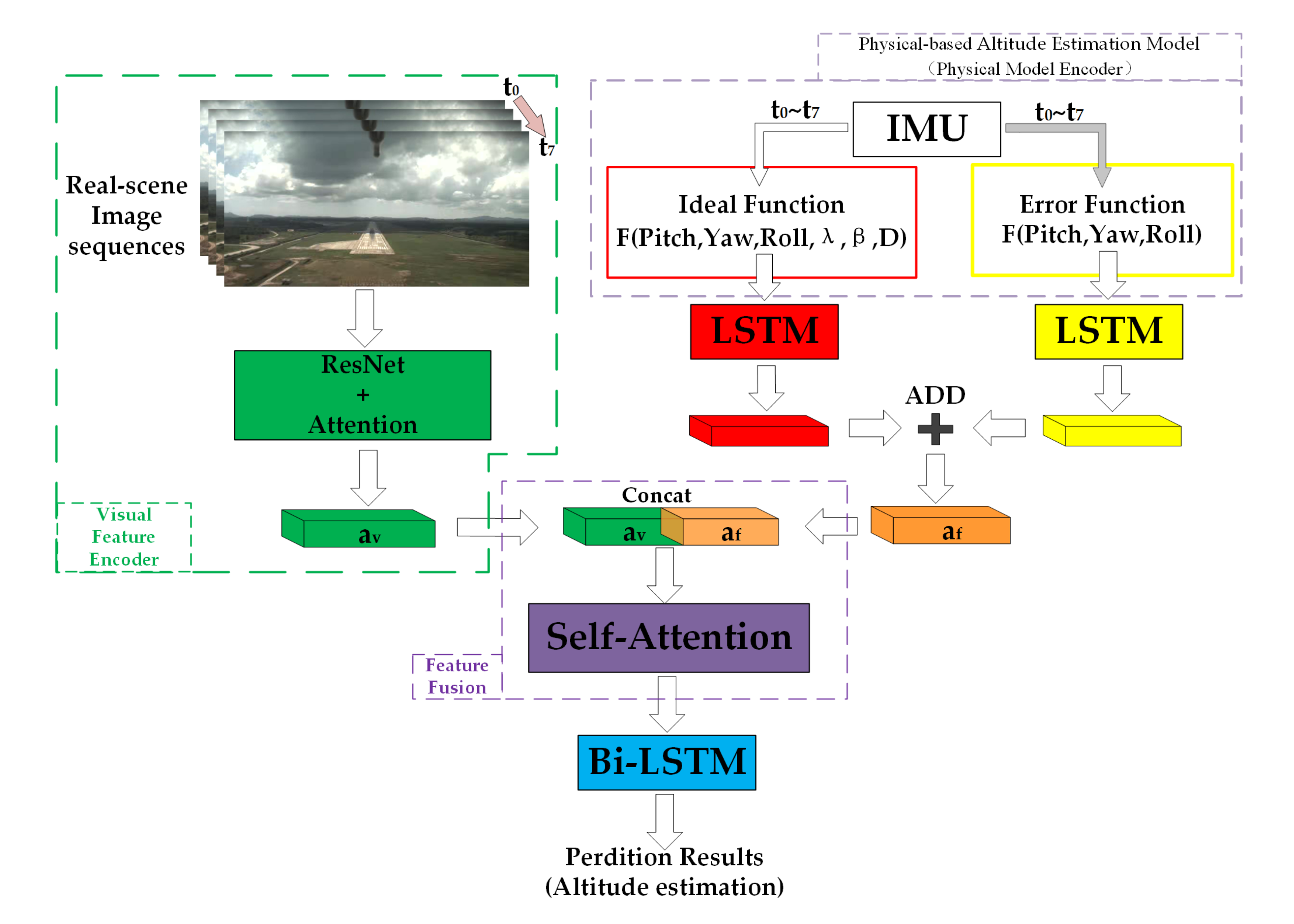
- We proposed a novel altitude estimation method that integrated a physical-based model into a deep neural network architecture to build a more robust and accurate altitude estimation model with visual and inertial data sequences. The current physical-based or learning-based methods cannot balance broad applications and performance, as well as data efficiency and a large requirement of training data. However, the physical reasoning we introduced into the network will be a driving stimulant, which can not only broaden the scope of applications and improve data efficiency of the CNN-LSTM-based altitude model, but also achieve a high-precision estimation for an extended range in various real scenarios.
- (2)
- Based on several appropriate assumptions, we designed a physical-based altitude model consisting of an image model of a monocular camera with kinematic principles. The model can not only ideally reveal the functional relations between the altitude values, the known information from sensors and their relations, but also simplify the training process by taking it as a part of the initial model of the neural network.
- (3)
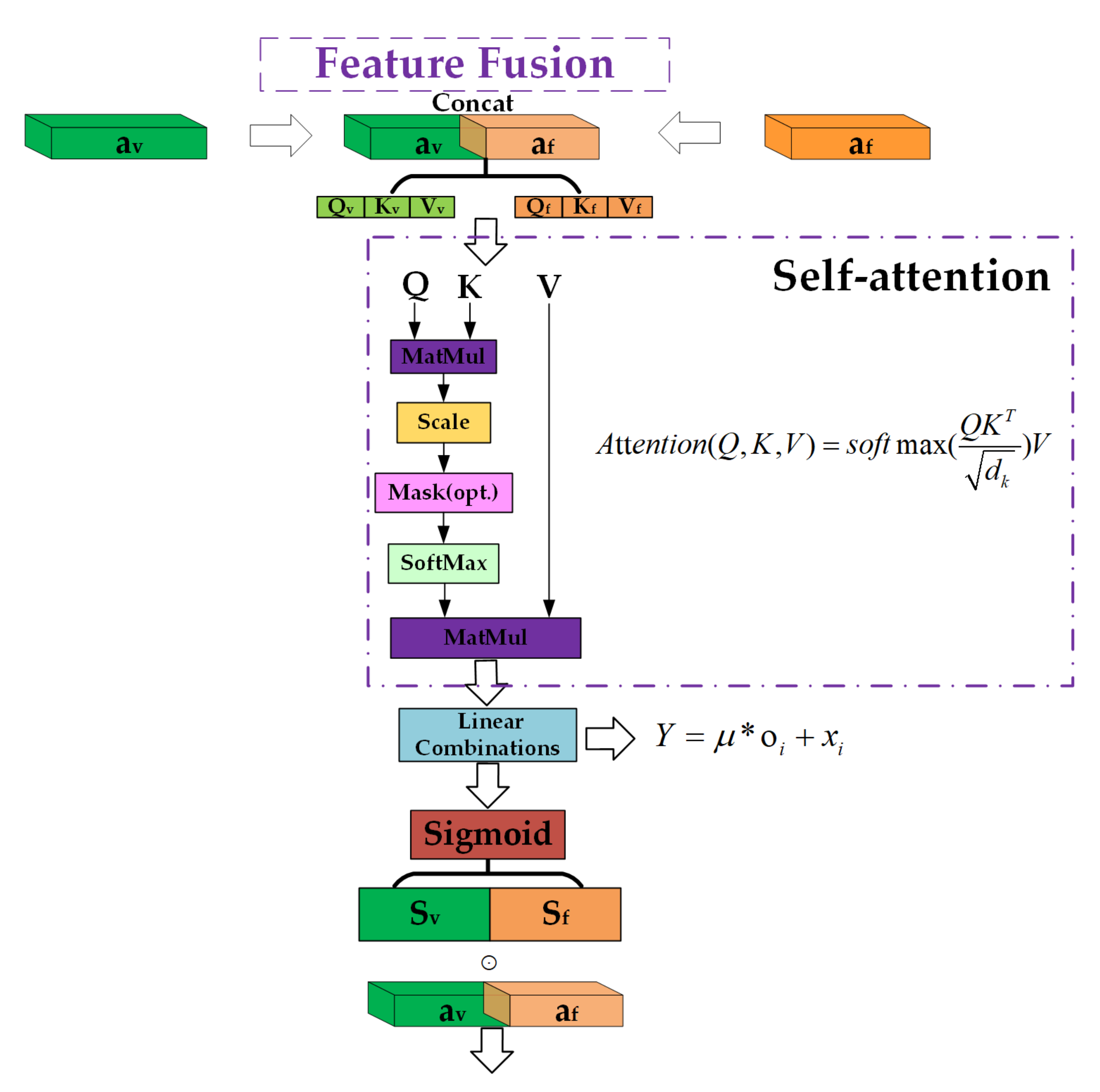
- We present a novel feature fusion module for the visual and inertial information, which uses a self-attention mechanism to map different features into the same feature space. Benefitting from this, the neural network can perceive the complex data association between the visual-inertial data sequences and the altitude model to improve the robustness and precision of the altitude estimation results.
2. Related Work
3. Materials and Methods
3.1. Physical-Based Altitude Estimation Model (Physical Model Encoder)
3.1.1. Ideal Function
- (1)
- The camera and IMU are located in the same location on the UAV, and the coordinate systems of these two sensors are coincident.
- (2)
- The camera position can represent the UAV position.
- (3)
- The runway can be observed completely on the image plane. The actual width is known and the bottom angles and can be obtained by the runway detection method.
- (4)
- The yaw angle is the relative angle between the UAV heading angle and the runway orientation angle.
3.1.2. Error Function
3.2. Visual Feature Encoder
3.3. Visual-Inertial Feature Fusion
3.4. Temporal Feature Extraction and Altitude Regression
3.5. Model Training
4. Results Comparisons and Analysis
4.1. Experimental Data and Metrics
4.2. Experimental Results and Analysis
5. Conclusions
6. Future Work
Author Contributions
Funding
Institutional Review Board Statement
Informed Consent Statement
Acknowledgments
Conflicts of Interest
References
- Templeton, T.; Shim, D.H.; Geyer, C.; Sastry, S.S. Autonomous vision-based landing and terrain mapping using an MPC-controlled unmanned rotorcraft. In Proceedings of the 2007 IEEE International Conference on Robotics and Automation, Rome, Italy, 10–14 April 2007; pp. 1349–1356. [Google Scholar]
- Mohammadi, A.; Feng, Y.; Zhang, C.; Rawashdeh, S.; Baek, S. Vision-based Autonomous Landing Using an MPC-controlled Micro UAV on a Moving Platform. In Proceedings of the 2020 International Conference on Unmanned Aircraft Systems (ICUAS), Athens, Greece, 1–4 September 2020; pp. 771–780. [Google Scholar]
- Nilsson, J.O.; Gupta, A.K.; Händel, P. Foot-mounted inertial navigation made easy. In Proceedings of the 2014 International Conference on Indoor Positioning and Indoor Navigation (IPIN), Busan, Korea, 27–30 October 2014; pp. 24–29. [Google Scholar]
- Siciliano, B.; Khatib, O. Springer Handbook of Robotics; Springer: Berlin/Heidelberg, Germany, 2016. [Google Scholar]
- Gautam, A.; Sujit, P.; Saripalli, S. A survey of autonomous landing techniques for UAVs. In Proceedings of the 2014 International Conference on Unmanned Aircraft Systems (ICUAS), Orlando, FL, USA, 27–30 May 2014; pp. 1210–1218. [Google Scholar]
- Araar, O.; Aouf, N.; Vitanov, I. Vision based autonomous landing of multirotor UAV on moving platform. J. Intell. Robot. Syst. 2017, 85, 369–384. [Google Scholar] [CrossRef]
- Strasdat, H.; Montiel, J.; Davison, A.J. Scale drift-aware large scale monocular SLAM. Robot. Sci. Syst. VI 2010, 2, 7. [Google Scholar]
- Choi, S.; Park, J.; Yu, W. Resolving scale ambiguity for monocular visual odometry. In Proceedings of the 2013 10th International Conference on Ubiquitous Robots and Ambient Intelligence (URAI), Jeju, Korea, 30 October–2 November 2013; pp. 604–608. [Google Scholar]
- Yang, Y.; Shen, Q.; Li, J.; Deng, Z.; Wang, H.; Gao, X. Position and attitude estimation method integrating visual odometer and GPS. Sensors 2020, 20, 2121. [Google Scholar] [CrossRef] [PubMed]
- Alvertos, N. Resolution limitations and error analysis for stereo camera models. In Proceedings of the Conference Proceedings ’88. IEEE Southeastcon, Knoxville, TN, USA, 10–13 April 1988; pp. 220–224. [Google Scholar]
- Gallup, D.; Frahm, J.M.; Mordohai, P.; Pollefeys, M. Variable baseline/resolution stereo. In Proceedings of the 2008 IEEE Conference on Computer Vision and Pattern Recognition, Anchorage, AK, USA, 23–28 June 2008; pp. 1–8. [Google Scholar]
- Hsu, T.S.; Wang, T.C. An improvement stereo vision images processing for object distance measurement. Int. J. Autom. Smart Technol. 2015, 5, 85–90. [Google Scholar]
- Luo, X.l.; Lv, J.H.; Sun, G. A visual-inertial navigation method for high-speed unmanned aerial vehicles. arXiv 2020, arXiv:2002.04791. [Google Scholar]
- Jung, Y.; Lee, D.; Bang, H. Close-range vision navigation and guidance for rotary UAV autonomous landing. In Proceedings of the 2015 IEEE International Conference on Automation Science and Engineering (CASE), Gothenburg, Sweden, 24–28 August 2015; pp. 342–347. [Google Scholar]
- Dagan, E.; Mano, O.; Stein, G.P.; Shashua, A. Forward collision warning with a single camera. In Proceedings of the IEEE Intelligent Vehicles Symposium 2004, Parma, Italy, 14–17 June 2004; pp. 37–42. [Google Scholar]
- Rosenbaum, D.; Gurman, A.; Samet, Y.; Stein, G.P.; Aloni, D. Pedestrian Collision Warning System. U.S. Patent 9,233,659, 15 March 2016. [Google Scholar]
- Arenado, M.I.; Oria, J.M.P.; Torre-Ferrero, C.; Rentería, L.A. Monovision-based vehicle detection, distance and relative speed measurement in urban traffic. IET Intell. Transp. Syst. 2014, 8, 655–664. [Google Scholar] [CrossRef]
- Saripalli, S.; Montgomery, J.F.; Sukhatme, G.S. Vision-based autonomous landing of an unmanned aerial vehicle. In Proceedings of the 2002 IEEE International Conference on Robotics and Automation (Cat. No. 02CH37292), Washington, DC, USA, 11–15 May 2002; Volume 3, pp. 2799–2804. [Google Scholar]
- Schmidt, T.; Hertkorn, K.; Newcombe, R.; Marton, Z.; Suppa, M.; Fox, D. Depth-based tracking with physical constraints for robot manipulation. In Proceedings of the 2015 IEEE International Conference on Robotics and Automation (ICRA), Seattle, WA, USA, 26–30 May 2015; pp. 119–126. [Google Scholar]
- Kolev, S.; Todorov, E. Physically consistent state estimation and system identification for contacts. In Proceedings of the 2015 IEEE-RAS 15th International Conference on Humanoid Robots (Humanoids), Seoul, Korea, 3–5 November 2015; pp. 1036–1043. [Google Scholar]
- Weiss, S.; Achtelik, M.W.; Lynen, S.; Chli, M.; Siegwart, R. Real-time onboard visual-inertial state estimation and self-calibration of mavs in unknown environments. In Proceedings of the 2012 IEEE International Conference on Robotics and Automation, Saint Paul, MN, USA, 14–18 May 2012; pp. 957–964. [Google Scholar]
- Jarry, G.; Delahaye, D.; Feron, E. Approach and landing aircraft on-board parameters estimation with lstm networks. In Proceedings of the 2020 International Conference on Artificial Intelligence and Data Analytics for Air Transportation (AIDA-AT), Singapore, 3–4 February 2020; pp. 1–6. [Google Scholar]
- Hou, H.; Xu, Q.; Lan, C.; Lu, W.; Zhang, Y.; Cui, Z.; Qin, J. UAV Pose Estimation in GNSS-Denied Environment Assisted by Satellite Imagery Deep Learning Features. IEEE Access 2020, 9, 6358–6367. [Google Scholar] [CrossRef]
- Mestav, K.R.; Luengo-Rozas, J.; Tong, L. Bayesian state estimation for unobservable distribution systems via deep learning. IEEE Trans. Power Syst. 2019, 34, 4910–4920. [Google Scholar] [CrossRef] [Green Version]
- Wu, J.; Yildirim, I.; Lim, J.J.; Freeman, B.; Tenenbaum, J. Galileo: Perceiving physical object properties by integrating a physics engine with deep learning. Adv. Neural Inf. Process. Syst. 2015, 28, 127–135. [Google Scholar]
- Jonschkowski, R.; Brock, O. Learning state representations with robotic priors. Auton. Robot. 2015, 39, 407–428. [Google Scholar] [CrossRef]
- Iten, R.; Metger, T.; Wilming, H.; Del Rio, L.; Renner, R. Discovering physical concepts with neural networks. Phys. Rev. Lett. 2020, 124, 010508. [Google Scholar] [CrossRef] [Green Version]
- Sünderhauf, N.; Brock, O.; Scheirer, W.; Hadsell, R.; Fox, D.; Leitner, J.; Upcroft, B.; Abbeel, P.; Burgard, W.; Milford, M.; et al. The limits and potentials of deep learning for robotics. Int. J. Robot. Res. 2018, 37, 405–420. [Google Scholar] [CrossRef] [Green Version]
- Chen, C.; Rosa, S.; Miao, Y.; Lu, C.X.; Wu, W.; Markham, A.; Trigoni, N. Selective sensor fusion for neural visual-inertial odometry. In Proceedings of the IEEE/CVF Conference on Computer Vision and Pattern Recognition, Long Beach, CA, USA, 15–20 June 2019; pp. 10542–10551. [Google Scholar]
- Dai, S.; Wu, Y. Motion from blur. In Proceedings of the 2008 IEEE Conference on Computer Vision and Pattern Recognition, Anchorage, AK, USA, 23–28 June 2008; pp. 1–8. [Google Scholar]
- Oktay, T.; Celik, H.; Turkmen, I. Maximizing autonomous performance of fixed-wing unmanned aerial vehicle to reduce motion blur in taken images. Proc. Inst. Mech. Eng. Part I J. Syst. Control Eng. 2018, 232, 857–868. [Google Scholar] [CrossRef]
- Kim, J.; Jung, Y.; Lee, D.; Shim, D.H. Outdoor autonomous landing on a moving platform for quadrotors using an omnidirectional camera. In Proceedings of the 2014 International Conference on Unmanned Aircraft Systems (ICUAS), Orlando, FL, USA, 27–30 May 2014; pp. 1243–1252. [Google Scholar]
- Wubben, J.; Fabra, F.; Calafate, C.T.; Krzeszowski, T.; Marquez-Barja, J.M.; Cano, J.C.; Manzoni, P. Accurate landing of unmanned aerial vehicles using ground pattern recognition. Electronics 2019, 8, 1532. [Google Scholar] [CrossRef] [Green Version]
- Rambach, J.R.; Tewari, A.; Pagani, A.; Stricker, D. Learning to fuse: A deep learning approach to visual-inertial camera pose estimation. In Proceedings of the 2016 IEEE International Symposium on Mixed and Augmented Reality (ISMAR), Merida, Mexico, 19–23 September 2016; pp. 71–76. [Google Scholar]
- Delmerico, J.; Scaramuzza, D. A benchmark comparison of monocular visual-inertial odometry algorithms for flying robots. In Proceedings of the 2018 IEEE International Conference on Robotics and Automation (ICRA), Brisbane, QLD, Australia, 21–25 May 2018; pp. 2502–2509. [Google Scholar]
- Leutenegger, S.; Lynen, S.; Bosse, M.; Siegwart, R.; Furgale, P. Keyframe-based visual–inertial odometry using nonlinear optimization. Int. J. Robot. Res. 2015, 34, 314–334. [Google Scholar] [CrossRef] [Green Version]
- Qin, T.; Li, P.; Shen, S. Vins-mono: A robust and versatile monocular visual-inertial state estimator. IEEE Trans. Robot. 2018, 34, 1004–1020. [Google Scholar] [CrossRef] [Green Version]
- Mourikis, A.I.; Roumeliotis, S.I. A multi-state constraint Kalman filter for vision-aided inertial navigation. In Proceedings of the 2007 IEEE International Conference on Robotics and Automation, Rome, Italy, 10–14 April 2007; pp. 3565–3572. [Google Scholar]
- Kaess, M.; Johannsson, H.; Roberts, R.; Ila, V.; Leonard, J.J.; Dellaert, F. iSAM2: Incremental smoothing and mapping using the Bayes tree. Int. J. Robot. Res. 2012, 31, 216–235. [Google Scholar] [CrossRef]
- Forster, C.; Carlone, L.; Dellaert, F.; Scaramuzza, D. IMU Preintegration on Manifold for Efficient Visual-Inertial Maximum-a-Posteriori Estimation; Georgia Institute of Technology: Atlanta, GA, USA, 2015. [Google Scholar]
- Clark, R.; Wang, S.; Wen, H.; Markham, A.; Trigoni, N. Vinet: Visual-inertial odometry as a sequence-to-sequence learning problem. In Proceedings of the AAAI Conference on Artificial Intelligence, San Francisco, CA, USA, 4–9 February 2017; Volume 31. [Google Scholar]
- Zhang, H.; Zhu, T. Aircraft Hard Landing Prediction Using LSTM Neural Network. In Proceedings of the 2nd International Symposium on Computer Science and Intelligent Control, Stockholm, Sweden, 21–23 September 2018; pp. 1–5. [Google Scholar]
- Wang, S.; Clark, R.; Wen, H.; Trigoni, N. Deepvo: Towards end-to-end visual odometry with deep recurrent convolutional neural networks. In Proceedings of the 2017 IEEE International Conference on Robotics and Automation (ICRA), Singapore, 29 May–3 June 2017; pp. 2043–2050. [Google Scholar]
- Jiao, J.; Jiao, J.; Mo, Y.; Liu, W.; Deng, Z. MagicVO: End-to-end monocular visual odometry through deep bi-directional recurrent convolutional neural network. arXiv 2018, arXiv:1811.10964. [Google Scholar]
- Han, L.; Lin, Y.; Du, G.; Lian, S. Deepvio: Self-supervised deep learning of monocular visual inertial odometry using 3D geometric constraints. In Proceedings of the 2019 IEEE/RSJ International Conference on Intelligent Robots and Systems (IROS), Macau, China, 3–8 November 2019; pp. 6906–6913. [Google Scholar]
- Vaswani, A.; Shazeer, N.; Parmar, N.; Uszkoreit, J.; Jones, L.; Gomez, A.N.; Kaiser, Ł.; Polosukhin, I. Attention is all you need. In Proceedings of the Advances in Neural Information Processing Systems, Long Beach, CA, USA, 4–9 December 2017; pp. 5998–6008. [Google Scholar]
- Zhang, H.; Goodfellow, I.; Metaxas, D.; Odena, A. Self-attention generative adversarial networks. In Proceedings of the International Conference on Machine Learning, PMLR, Long Beach, CA, USA, 9–15 June 2019; pp. 7354–7363. [Google Scholar]
- Donahue, J.; Anne Hendricks, L.; Guadarrama, S.; Rohrbach, M.; Venugopalan, S.; Saenko, K.; Darrell, T. Long-term recurrent convolutional networks for visual recognition and description. In Proceedings of the IEEE Conference on Computer Vision and Pattern Recognition, Boston, MA, USA, 7–12 June 2015; pp. 2625–2634. [Google Scholar]
- Khor, H.Q.; See, J.; Phan, R.C.W.; Lin, W. Enriched long-term recurrent convolutional network for facial micro-expression recognition. In Proceedings of the 2018 13th IEEE International Conference on Automatic Face & Gesture Recognition (FG 2018), Xi’an, China, 15–19 May 2018; pp. 667–674. [Google Scholar]
- Woo, S.; Park, J.; Lee, J.Y.; Kweon, I.S. Cbam: Convolutional block attention module. In Proceedings of the European Conference on Computer Vision (ECCV), Munich, Germany, 8–14 September 2018; pp. 3–19. [Google Scholar]
- He, K.; Zhang, X.; Ren, S.; Sun, J. Deep residual learning for image recognition. In Proceedings of the IEEE Conference on Computer Vision and Pattern Recognition, Las Vegas, NV, USA, 26 June–1 July 2016; pp. 770–778. [Google Scholar]
- Deng, J.; Dong, W.; Socher, R.; Li, L.J.; Li, K.; Fei-Fei, L. Imagenet: A large-scale hierarchical image database. In Proceedings of the 2009 IEEE Conference on Computer Vision and Pattern Recognition, Miami, FL, USA, 20–25 June 2009; pp. 248–255. [Google Scholar]
- Almalioglu, Y.; Turan, M.; Sari, A.E.; Saputra, M.R.U.; de Gusmão, P.P.; Markham, A.; Trigoni, N. Selfvio: Self-supervised deep monocular visual-inertial odometry and depth estimation. arXiv 2019, arXiv:1911.09968. [Google Scholar]
- Eling, C.; Klingbeil, L.; Kuhlmann, H. Development of an RTK-GPS System for Precise Real-Time Positioning of Lightweight UAVs; Herbert Wichmann Verlag: Karlsruhe, Germany, 2014. [Google Scholar]
- Langley, R.B. RTK GPS. GPS World 1998, 9, 70–76. [Google Scholar]
- Anitha, G.; Kumar, R.G. Vision based autonomous landing of an unmanned aerial vehicle. Procedia Eng. 2012, 38, 2250–2256. [Google Scholar] [CrossRef] [Green Version]
- Redmon, J.; Divvala, S.; Girshick, R.; Farhadi, A. You only look once: Unified, real-time object detection. In Proceedings of the IEEE Conference on Computer Vision and Pattern Recognition, Las Vegas, NV, USA, 26 June–1 July 2016; pp. 779–788. [Google Scholar]
- Xue, N.; Bai, S.; Wang, F.; Xia, G.S.; Wu, T.; Zhang, L. Learning attraction field representation for robust line segment detection. In Proceedings of the IEEE/CVF Conference on Computer Vision and Pattern Recognition, Long Beach, CA, USA, 16–20 June 2019; pp. 1595–1603. [Google Scholar]


| Method | Physical-Based | Learning-Based |
|---|---|---|
| Good generality | Highly accurate in trained regime | |
| Advantage | Physics are universal | Highly robust in trained regime |
| Data efficient | Require little priors | |
| Require strong priors assumption | Require large amount of data | |
| Disadvantage | Require good modeling | Risk of overfitting |
| Hardly achieve better accuracy | Generality only in trained regime |
| Method | MAE (m) | RMSE | |
|---|---|---|---|
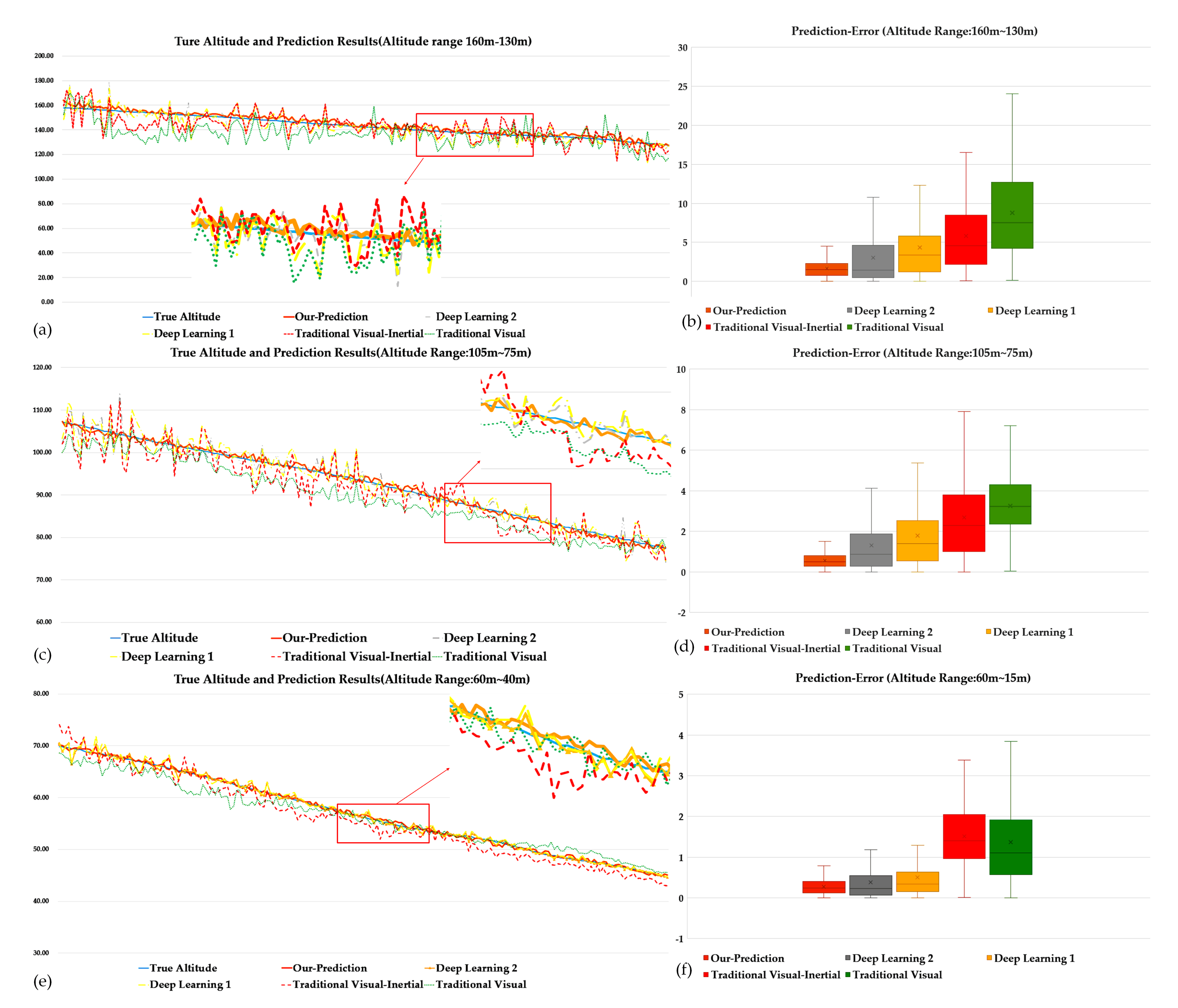
| Traditional Visual [56] | 7.6760 | 11.1068 | −1.1551 |
| Traditional Visual-Inertial [36] | 6.0696 | 9.4284 | −0.5157 |
| Deep Learning 1 [44] | 3.9028 | 5.1624 | 0.5954 |
| Deep Learning 2 [41] | 3.1246 | 4.1994 | 0.7327 |
| Our Method | 1.0567 | 1.1866 | 0.9679 |
| Method | MAE (m) | RMSE | |
|---|---|---|---|
| Traditional Visual [56] | 5.9274 | 6.6192 | 0.5763 |
| Traditional Visual-Inertial [36] | 3.2191 | 3.8659 | 0.7414 |
| Deep Learning 1 [44] | 1.7654 | 2.5537 | 0.8985 |
| Deep Learning 2 [41] | 1.3243 | 2.1242 | 0.9288 |
| Our Method | 0.3402 | 0.4688 | 0.9961 |
| Method | MAE (m) | RMSE | |
|---|---|---|---|
| Traditional Visual [56] | 1.7055 | 2.0385 | 0.9189 |
| Traditional Visual-Inertial [36] | 4.4189 | 4.0917 | 0.6754 |
| Deep Learning 1 [44] | 0.4303 | 0.6304 | 0.9921 |
| Deep Learning 2 [41] | 0.3443 | 0.5287 | 0.9961 |
| Our Method | 0.1368 | 0.1715 | 0.9993 |
Publisher’s Note: MDPI stays neutral with regard to jurisdictional claims in published maps and institutional affiliations. |
© 2021 by the authors. Licensee MDPI, Basel, Switzerland. This article is an open access article distributed under the terms and conditions of the Creative Commons Attribution (CC BY) license (https://creativecommons.org/licenses/by/4.0/).
Share and Cite
Zhang, X.; He, Z.; Ma, Z.; Jun, P.; Yang, K. VIAE-Net: An End-to-End Altitude Estimation through Monocular Vision and Inertial Feature Fusion Neural Networks for UAV Autonomous Landing. Sensors 2021, 21, 6302. https://doi.org/10.3390/s21186302
Zhang X, He Z, Ma Z, Jun P, Yang K. VIAE-Net: An End-to-End Altitude Estimation through Monocular Vision and Inertial Feature Fusion Neural Networks for UAV Autonomous Landing. Sensors. 2021; 21(18):6302. https://doi.org/10.3390/s21186302
Chicago/Turabian StyleZhang, Xupei, Zhanzhuang He, Zhong Ma, Peng Jun, and Kun Yang. 2021. "VIAE-Net: An End-to-End Altitude Estimation through Monocular Vision and Inertial Feature Fusion Neural Networks for UAV Autonomous Landing" Sensors 21, no. 18: 6302. https://doi.org/10.3390/s21186302
APA StyleZhang, X., He, Z., Ma, Z., Jun, P., & Yang, K. (2021). VIAE-Net: An End-to-End Altitude Estimation through Monocular Vision and Inertial Feature Fusion Neural Networks for UAV Autonomous Landing. Sensors, 21(18), 6302. https://doi.org/10.3390/s21186302