
Improved 2D Ground Target Tracking in GPS-Based Passive Radar Scenarios

 , , , and
Abstract
:
1. Introduction
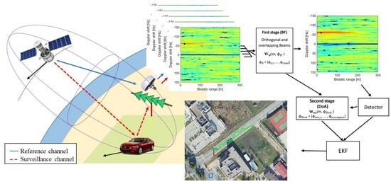
2. System Operation Principle
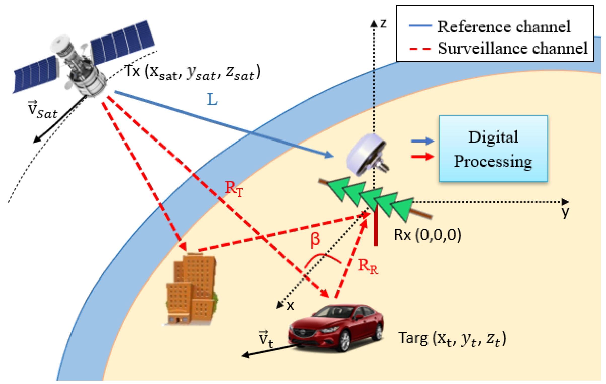
2.1. GPS Passive Radar Geometry
2.2. GPS Passive Radar Signal Processing
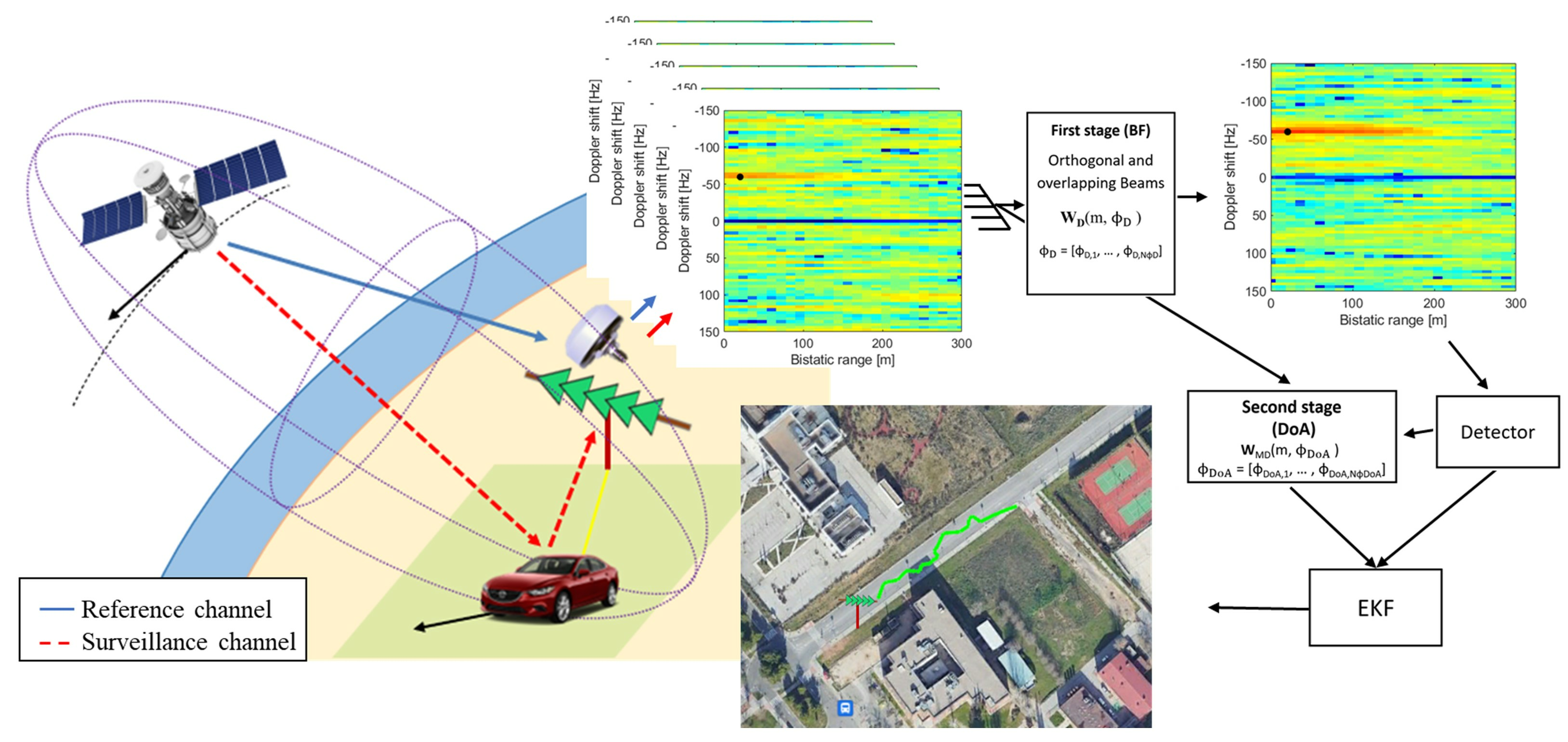
3. Ground Target 2D Localization Scheme
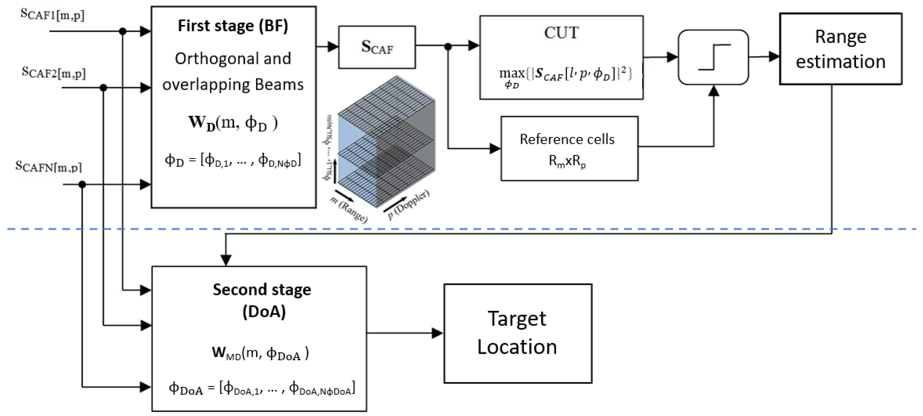
3.1. First Stage Spatial Filtering
- To form the first set of simultaneous beams, digital beamforming techniques were selected under the requirement of sidelobe level control to generate orthogonal beams along with the azimuth sector of the single radiating element. An iterative process was followed to define the N orthogonal beam steering angles, . The process starts with the first lobe steered to the broadside, then the steering direction of the adjacent lobes is adjusted to the first null of the initial beam. The process continues with the following adjacent lobes until the entire azimuthal sector of a single radiating element is covered.
- The orthogonal beams design procedure reduces the contribution to signal power in the current beam of targets whose DoAs are the steering directions of adjacent beams. However, the decrease in gain with respect to the maximum at the intersection points of the beams can be greater than 3 dB, negatively affecting the echoes of the targets in those directions (Figure 4). As the main objective of this first stage of spatial filtering is to improve target echoes SNR to allow their detection, beamforming gain losses should be minimized along the whole coverage area. Therefore, a second set of N − 1 steering angles, , was defined according to the crossing points of the previous orthogonal beams. Both steering angle sets are merged together in a steering vector to continue the design process, .
- The optimization problem was solved for each steering direction and Doppler shift pair (,p) to compute the weight vector . Applying the weight vectors to the corresponding snapshots in the transformed domain (6), a three dimensional matrix, is obtained.
3.2. Detection Stage
3.3. Second Stage Spatial Filtering
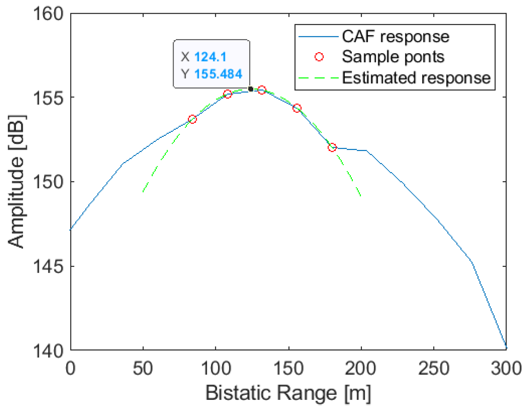
3.4. Target Localization
3.5. Estimation of the Initial Target Velocity
4. Target Tracking
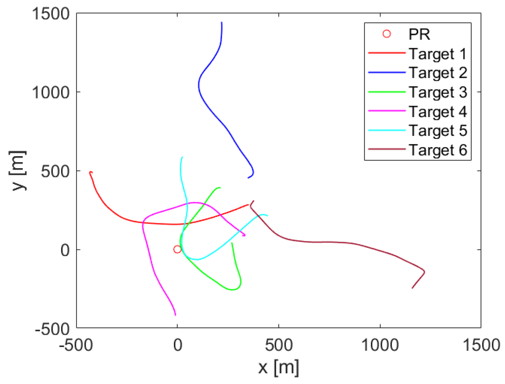
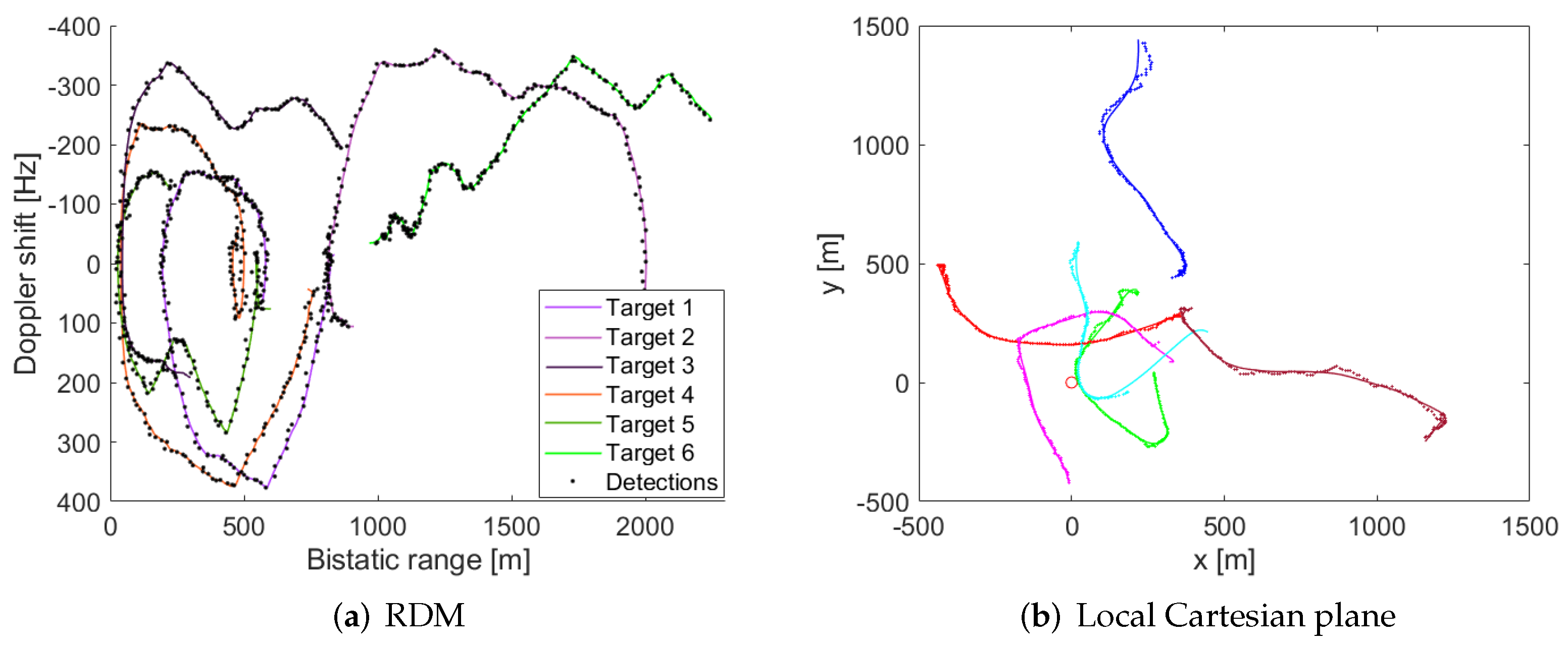
5. Simulation Results
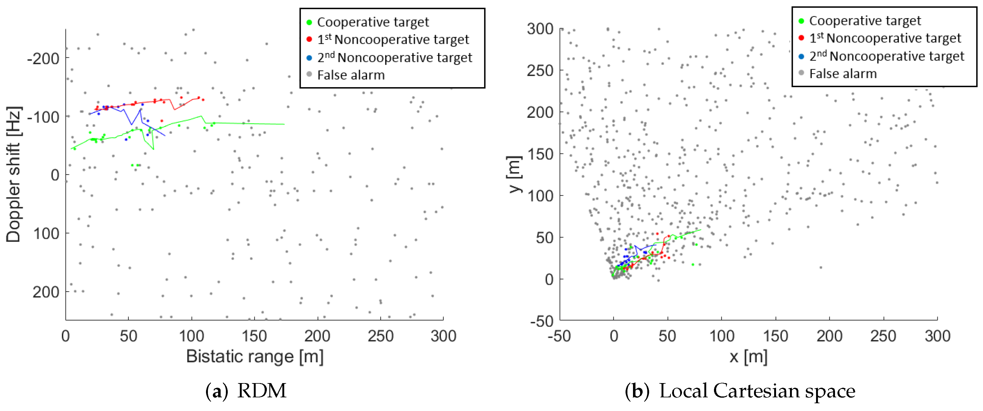
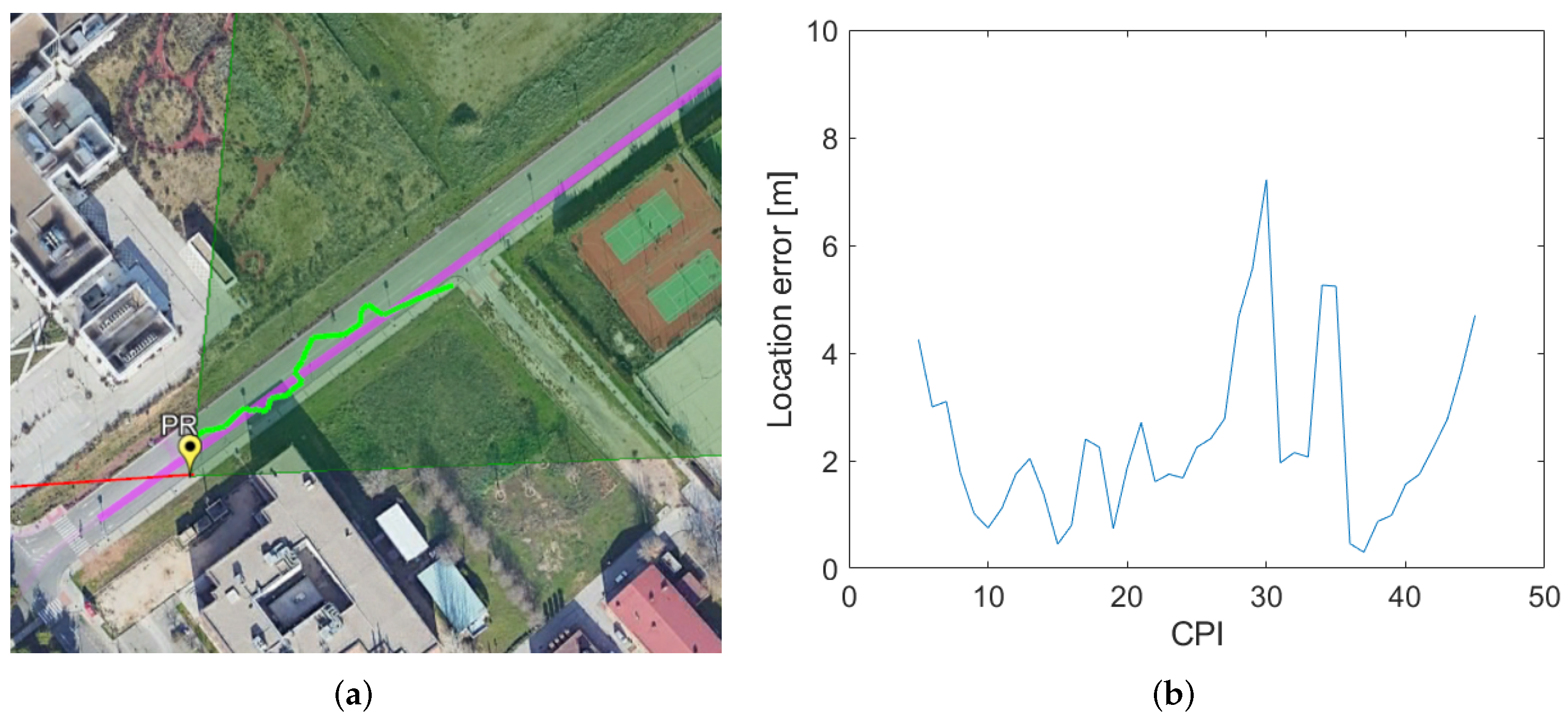
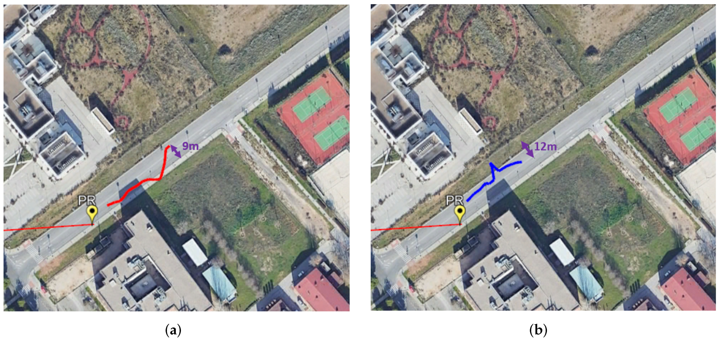
6. Results with Real Data
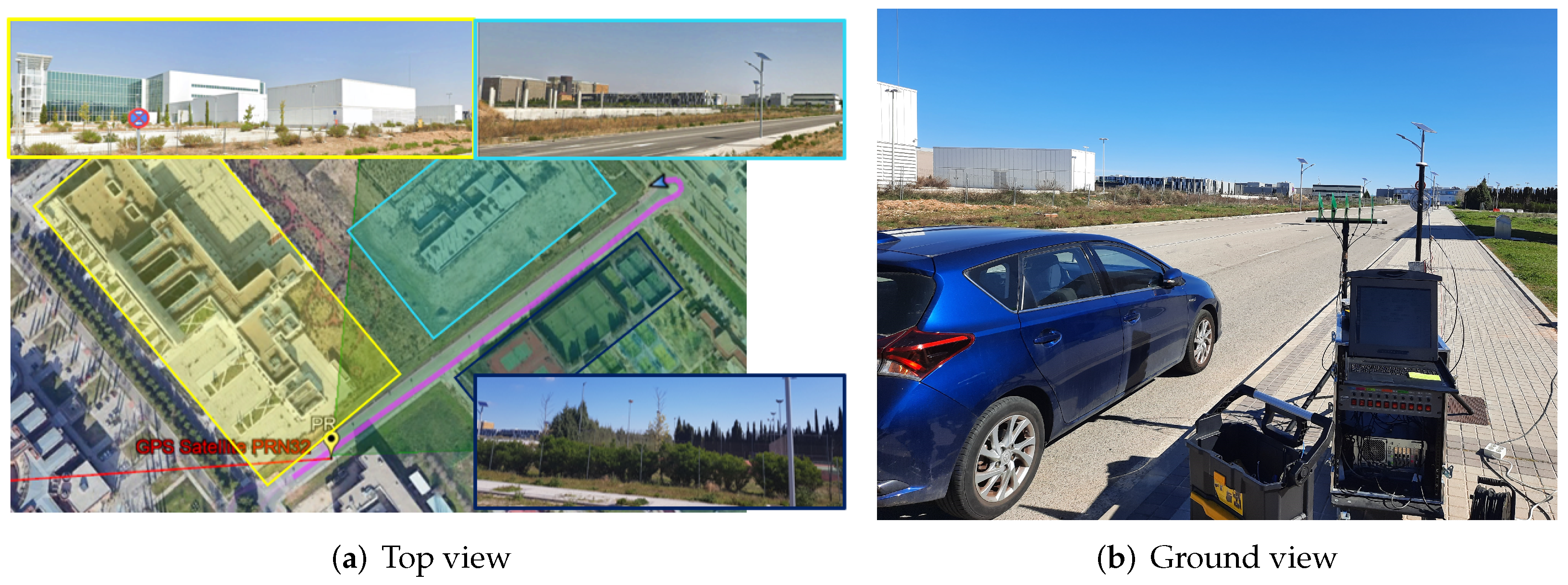
6.1. Radar Scenario
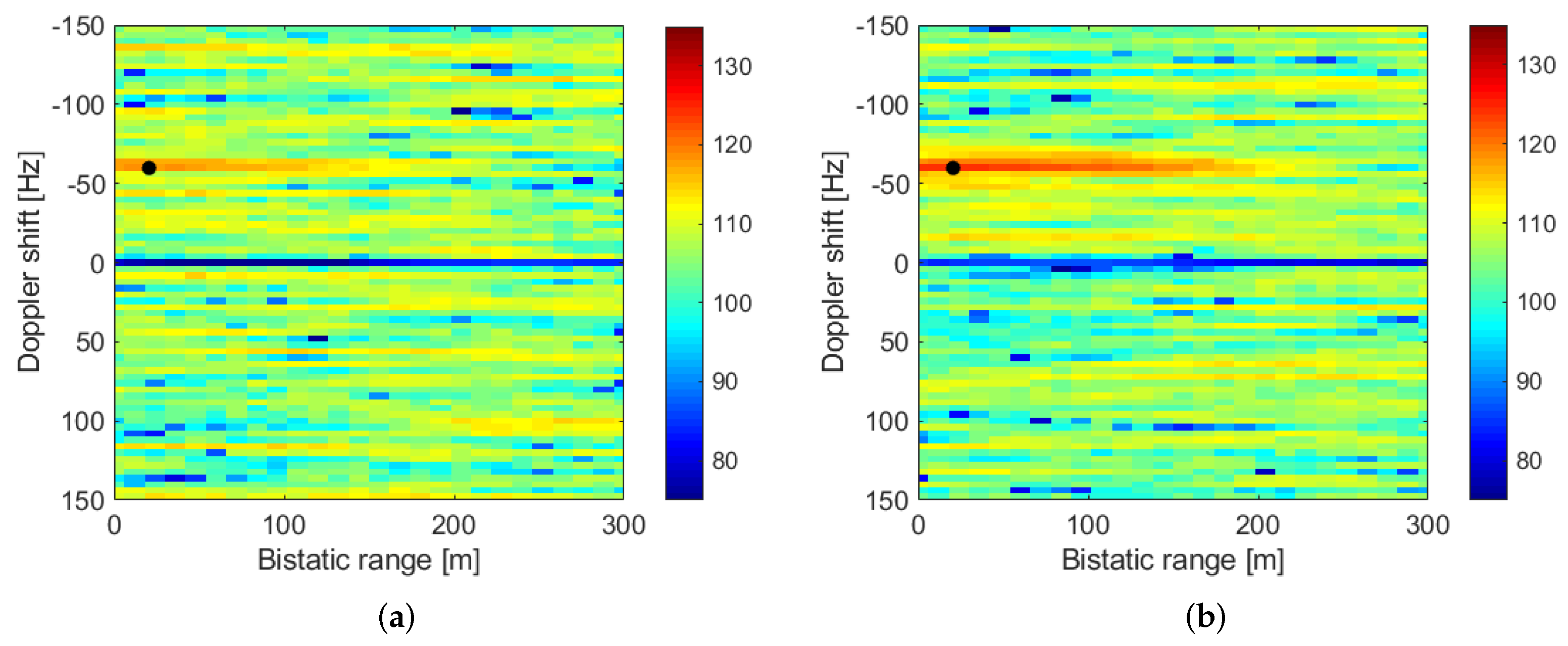
6.2. Results
7. Conclusions
Author Contributions
Funding
Institutional Review Board Statement
Informed Consent Statement
Conflicts of Interest
References
- IEEE Std 686-2017 (Revision of IEEE Std 686-2008); IEEE Standard for Radar Definitions. IEEE: Manhattan, NY, USA, 2017; pp. 1–54.
- Malanowski, M.; Kulpa, K.; Misjurewicz, J. PaRaDe—Passive Radar Demostrator family development at Warsaw University of Technology. In Proceedings of the Microwaves, Radar and Remote Sensing Symposium, Kiev, Ukraine, 22–24 September 2008; pp. 75–78. [Google Scholar]
- Kłos, J.; Droszcz, A.; Jędrzejewski, K.; Kulpa, K.; Pozoga, M. On the Possibility of Using LOFAR Radio Telescope for Passive Radiolocation. In Proceedings of the 21st International Radar Symposium (IRS), Warsaw, Poland, 5–8 October 2020; pp. 73–76. [Google Scholar] [CrossRef]
- Plotka, M.; Malanowski, M.; Samczynski, P.; Kulpa, K.; Abratkiewicz, K. Passive Bistatic Radar Based on VHF DVB-T Signal. In Proceedings of the 2020 IEEE International Radar Conference (RADAR), Washington, DC, USA, 28–30 April 2020; pp. 596–600. [Google Scholar] [CrossRef]
- Blazquez-Garcia, R.; Casamayon-Anton, J.; Burgos-Garcia, M. LTE-R Based Passive Multistatic Radar for High-Speed Railway Network Surveillance. In Proceedings of the 15th European Radar Conference (EuRAD), Madrid, Spain, 26–28 September 2018; pp. 6–9. [Google Scholar] [CrossRef]
- Cherniakov, M. Experiences Gained during the Development of a Passive BSAR with GNSS Transmitters of Opportunity. Int. J. Navig. Obs. 2008, 2008, 807958. [Google Scholar] [CrossRef]
- Rosado-Sanz, J.; Jarabo-Amores, M.P.; Mata-Moya, D.; Gómez-del-Hoyo, P.J.; Del-Rey-Maestre, N. Contoured-beam reflectarray for improving angular coverage in DVB-S passive radars. In Proceedings of the 20th International Radar Symposium (IRS), Ulm, Germany, 26–28 June 2019; pp. 1–8. [Google Scholar]
- Ummenhofer, M.; Lavau, L.C.; Cristallini, D.; O’Hagan, D. UAV Micro-Doppler Signature Analysis Using DVB-S Based Passive Radar. In Proceedings of the 2020 IEEE International Radar Conference (RADAR), Washington, DC, USA, 28–30 April 2020; pp. 1007–1012. [Google Scholar]
- Nasso, I.; Santi, F.; Pastina, D. Ship target velocity estimation with multi-transmitter GNSS-based. In Proceedings of the 21st International Radar Symposium (IRS), Berlin, Germany, 21–22 June 2021; pp. 1–10. [Google Scholar] [CrossRef]
- Ma, H.; Antoniou, M.; Cherniakov, M.; Pastina, D.; Santi, F.; Pieralice, F.; Bucciarelli, M. Maritime target detection using GNSS-based radar: Experimental proof of concept. In Proceedings of the 2017 IEEE Radar Conference (RadarConf), Seattle, WA, USA, 8–12 May 2017; pp. 464–469. [Google Scholar] [CrossRef]
- Santi, F.; Pastina, D.; Bucciarelli, M. Maritime moving target detection technique for passive bistatic radar with GNSS transmitters. In Proceedings of the 18th International Radar Symposium (IRS), Munich, Germany, 28–30 June 2017; pp. 1–10. [Google Scholar] [CrossRef]
- Huang, C.; Li, Z.; Lou, M.; Qiu, X.; An, H.; Wu, J.; Yang, J.; Huang, W. BeiDou-Based Passive Radar Vessel Target Detection: Method and Experiment via Long-Time Optimized Integration. Remote Sens. 2021, 13, 3933. [Google Scholar] [CrossRef]
- Suberviola, I.; Mayordomo, I.; Mendizabal, J. Experimental Results of Air Target Detection with a GPS Forward-Scattering Radar. IEEE Geosci. Remote Sens. Lett. 2012, 9, 47–51. [Google Scholar] [CrossRef]
- Gronowski, K.; Samczynski, P.; Stasiak, K.; Kulpa, K. First results of air target detection using single channel passive radar utilizing GPS illumination. In Proceedings of the 2019 IEEE Radar Conference (RadarConf), Boston, MA, USA, 22–26 April 2019; pp. 1–6. [Google Scholar] [CrossRef]
- Gomez-del-Hoyo, P.; Jarabo-Amores, M.; Mata-Moya, D.; del-Rey-Maestre, N.; Rosado-Sanz, J. First Approach on Ground Target Detection with GPS based Passive Radar: Experimental Results. In Proceedings of the 2019 Signal Processing Symposium (SPSympo), Krakow, Poland, 17–19 September 2019; pp. 71–75. [Google Scholar]
- Gomez-del-Hoyo, P.; Jarabo-Amores, M.; Mata-Moya, D.; del-Rey-Maestre, N.; Rosado-Sanz, J. 2D Ground Target Location Using GPS based Passive Radar. In Proceedings of the 2021 Signal Processing Symposium (SPSympo), Lodz, Poland, 17–19 September 2021; pp. 81–86. [Google Scholar]
- Jarabo-Amores, M.P.; Bárcena-Humanes, J.L.; Gomez-del Hoyo, P.J.; del Rey-Maestre, N.; Juara-Casero, D.; Gaitán-Cabañas, F.J.; Mata-Moya, D. IDEPAR: A multichannel digital video broadcasting-terrestrial passive radar technological demonstrator in terrestrial radar scenarios. IET Radar Sonar Navig. 2017, 11, 1–9. [Google Scholar] [CrossRef]
- Tsui, J.B.Y. Fundamentals of Global Positioning System Receivers: A Software Approach; John Wiley & Sons, Inc.: Hoboken, NJ, USA, 2005. [Google Scholar]
- Cardinali, R.; Colone, F.; Ferretti, C.; Lombardo, P. Comparison of clutter and multipath cancellation techniques for passive radar. In Proceedings of the IEEE Radar Conference, Waltham, MA, USA, 17–20 April 2007; Volume 1, pp. 469–474. [Google Scholar]
- del Rey-Maestre, N.; Mata-Moya, D.; Jarabo-Amores, M.P.; Gómez-del Hoyo, P.J.; Bárcena-Humanes, J.L.; Rosado-Sanz, J. Passive Radar Array Processing with Non-Uniform Linear Arrays for Ground Target’s Detection and Localization. Remote Sens. 2017, 9, 756. [Google Scholar] [CrossRef]
- Malanowski, M.P. Signal Processing for Passive Bistatic Radar; Artech-House: Norwood, MA, USA, 2019. [Google Scholar]
- Kalman, R. A new approach to linear filtering and prediction problems. J. Basic Eng. 1960, 82, 35–45. [Google Scholar] [CrossRef]
- Malanowski, M.; Kulpa, K. Two Methods for Target Localization in Multistatic Passive Radar. IEEE Trans. Aerosp. Electron. Syst. 2012, 48, 572–580. [Google Scholar] [CrossRef]
- Li, J.; Zhao, Y.; Li, D. Accurate single-observer passive coherent location estimation based on TDOA and DOA. Chin. J. Aeronaut. 2014, 27, 913–923. [Google Scholar] [CrossRef]
- Ummenhofer, M.; Kohler, M.; Schell, J.; O’Hagan, D.W. Direction of Arrival Estimation Techniques for Passive Radar based 3D Target Localization. In Proceedings of the 2019 IEEE Radar Conference (RadarConf), Boston, MA, USA, 22–26 April 2019; pp. 1–6. [Google Scholar]
- Rong Li, X.; Jilkov, V.P. Survey of maneuvering target tracking. Part I. Dynamic models. IEEE Trans. Aerosp. Electron. Syst. 2003, 39, 1333–1364. [Google Scholar] [CrossRef]
- Welch, G.; Bishop, G. An Introduction to the Kalman Filter. Technical Report TR 95-041, University of North Carolina at Chapel Hill. 24 July 2006. Available online: https://www.cs.unc.edu/~welch/media/pdf/kalman_intro.pdf (accessed on 29 December 2021).


| Simulated Data | Real Data | |||||||
|---|---|---|---|---|---|---|---|---|
| Targ 1 | Targ 2 | Targ 3 | Targ 4 | Targ 5 | Targ 6 | Total | Coop. Targ | |
| [m] | 4.44 | 10.76 | 6.65 | 2.96 | 3.09 | 11.19 | 7.46 | 2.38 |
| [m] | 3.5 | 10.76 | 5.57 | 7.86 | 5.38 | 9.31 | 7.77 | 1.58 |
Publisher’s Note: MDPI stays neutral with regard to jurisdictional claims in published maps and institutional affiliations. |
© 2022 by the authors. Licensee MDPI, Basel, Switzerland. This article is an open access article distributed under the terms and conditions of the Creative Commons Attribution (CC BY) license (https://creativecommons.org/licenses/by/4.0/).
Share and Cite
Gomez-del-Hoyo, P.; del-Rey-Maestre, N.; Jarabo-Amores, M.-P.; Mata-Moya, D.; Benito-Ortiz, M.-d.-C. Improved 2D Ground Target Tracking in GPS-Based Passive Radar Scenarios. Sensors 2022, 22, 1724. https://doi.org/10.3390/s22051724
Gomez-del-Hoyo P, del-Rey-Maestre N, Jarabo-Amores M-P, Mata-Moya D, Benito-Ortiz M-d-C. Improved 2D Ground Target Tracking in GPS-Based Passive Radar Scenarios. Sensors. 2022; 22(5):1724. https://doi.org/10.3390/s22051724
Chicago/Turabian StyleGomez-del-Hoyo, Pedro, Nerea del-Rey-Maestre, María-Pilar Jarabo-Amores, David Mata-Moya, and María-de-Cortés Benito-Ortiz. 2022. "Improved 2D Ground Target Tracking in GPS-Based Passive Radar Scenarios" Sensors 22, no. 5: 1724. https://doi.org/10.3390/s22051724
APA StyleGomez-del-Hoyo, P., del-Rey-Maestre, N., Jarabo-Amores, M.-P., Mata-Moya, D., & Benito-Ortiz, M.-d.-C. (2022). Improved 2D Ground Target Tracking in GPS-Based Passive Radar Scenarios. Sensors, 22(5), 1724. https://doi.org/10.3390/s22051724