
Deep Q-Learning-Based Transmission Power Control of a High Altitude Platform Station with Spectrum Sharing

 , , and
Abstract
:1. Introduction
1.1. Related Works
1.2. Contributions
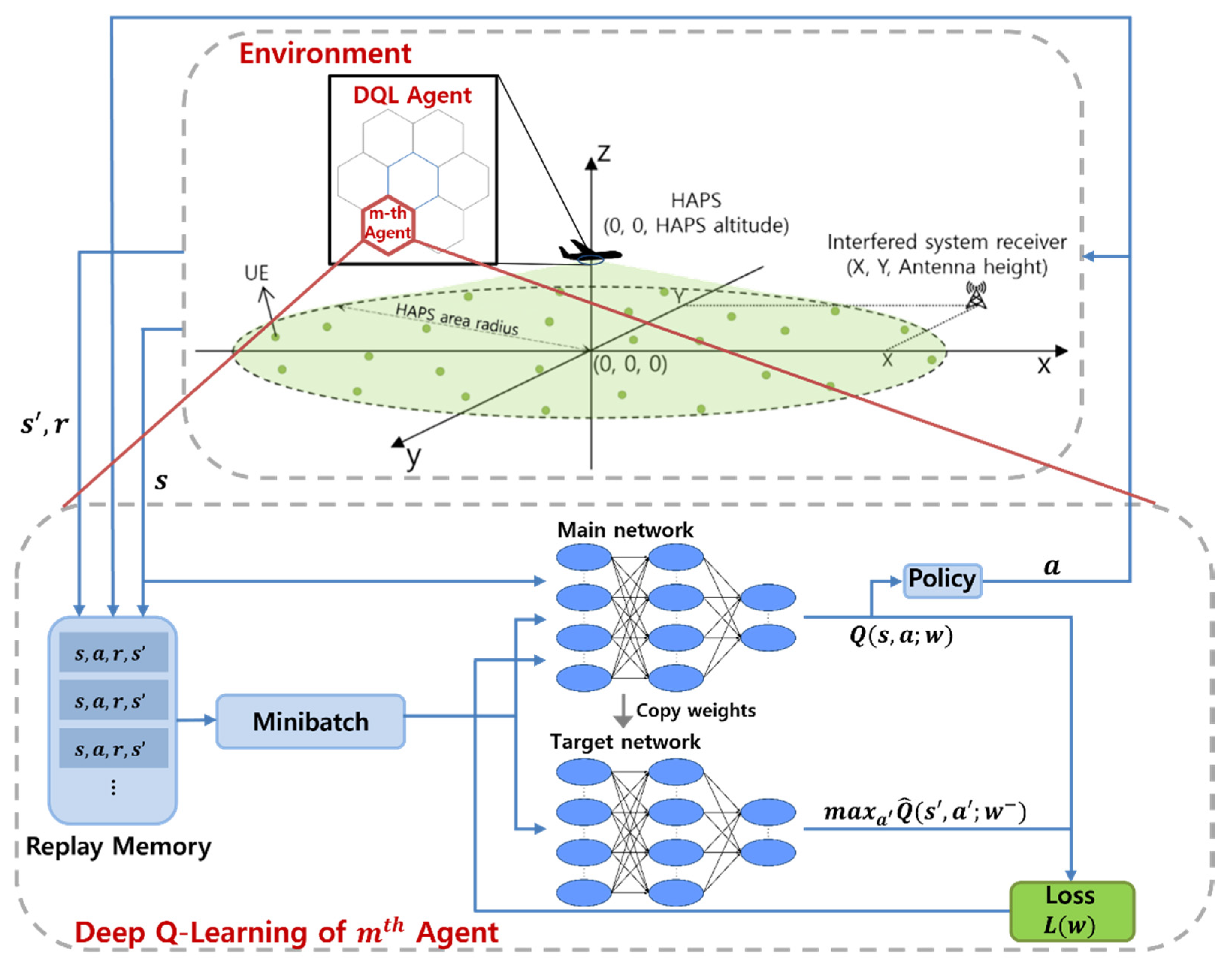
2. System Model
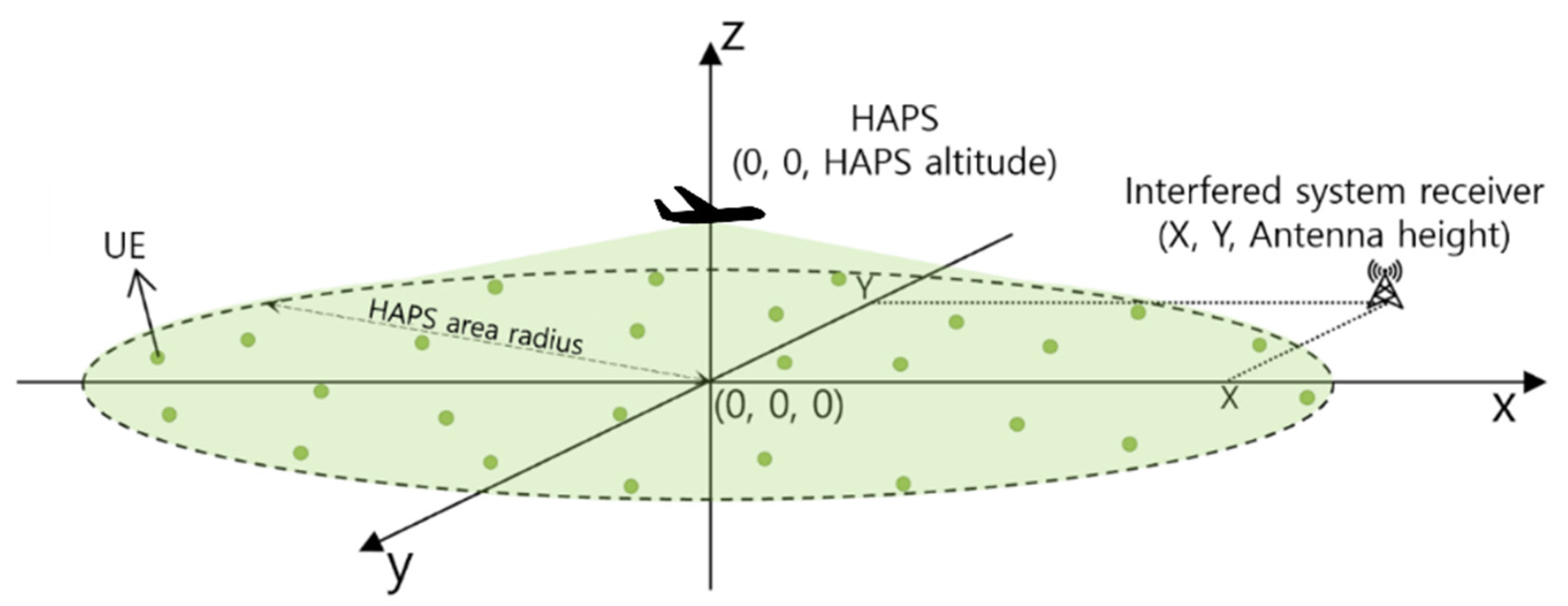
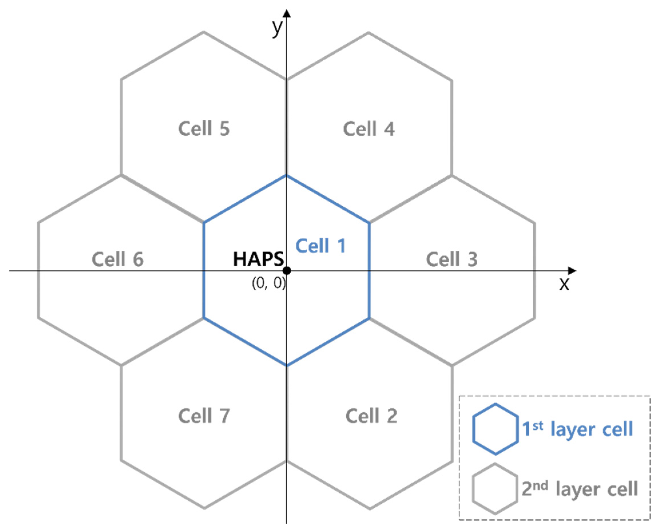
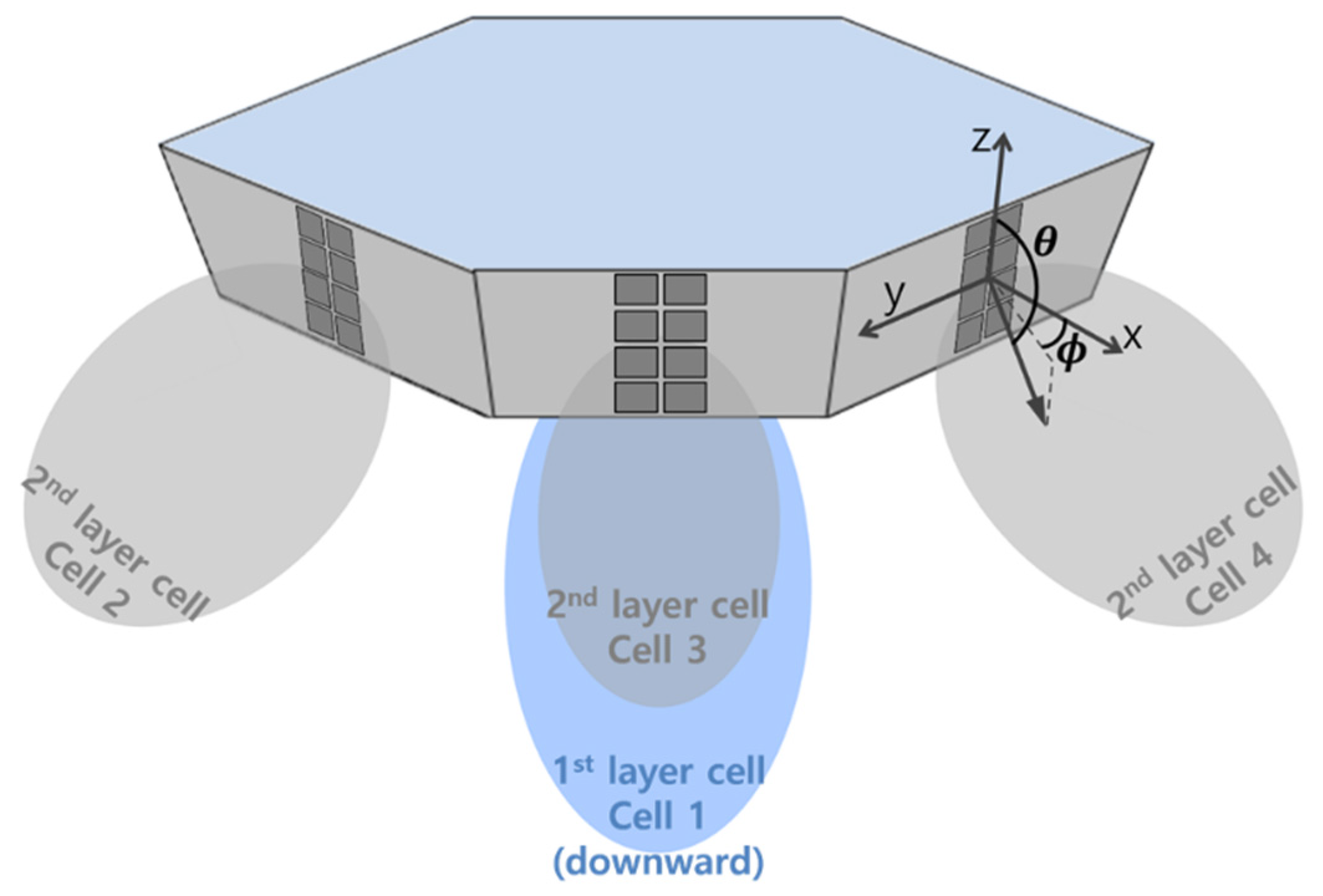
2.1. System Deployment Model
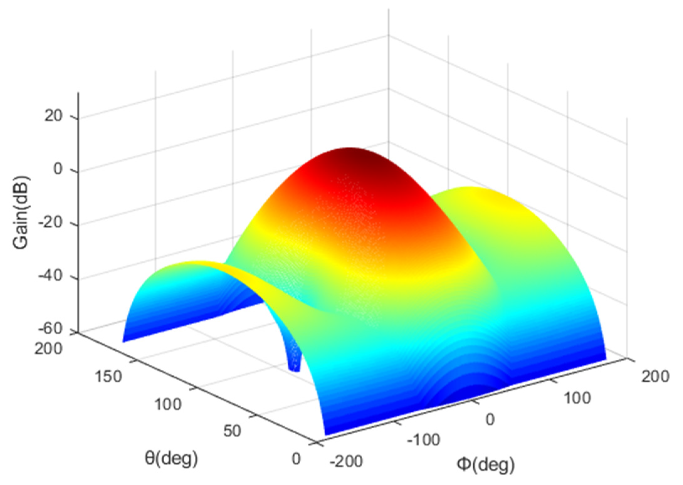
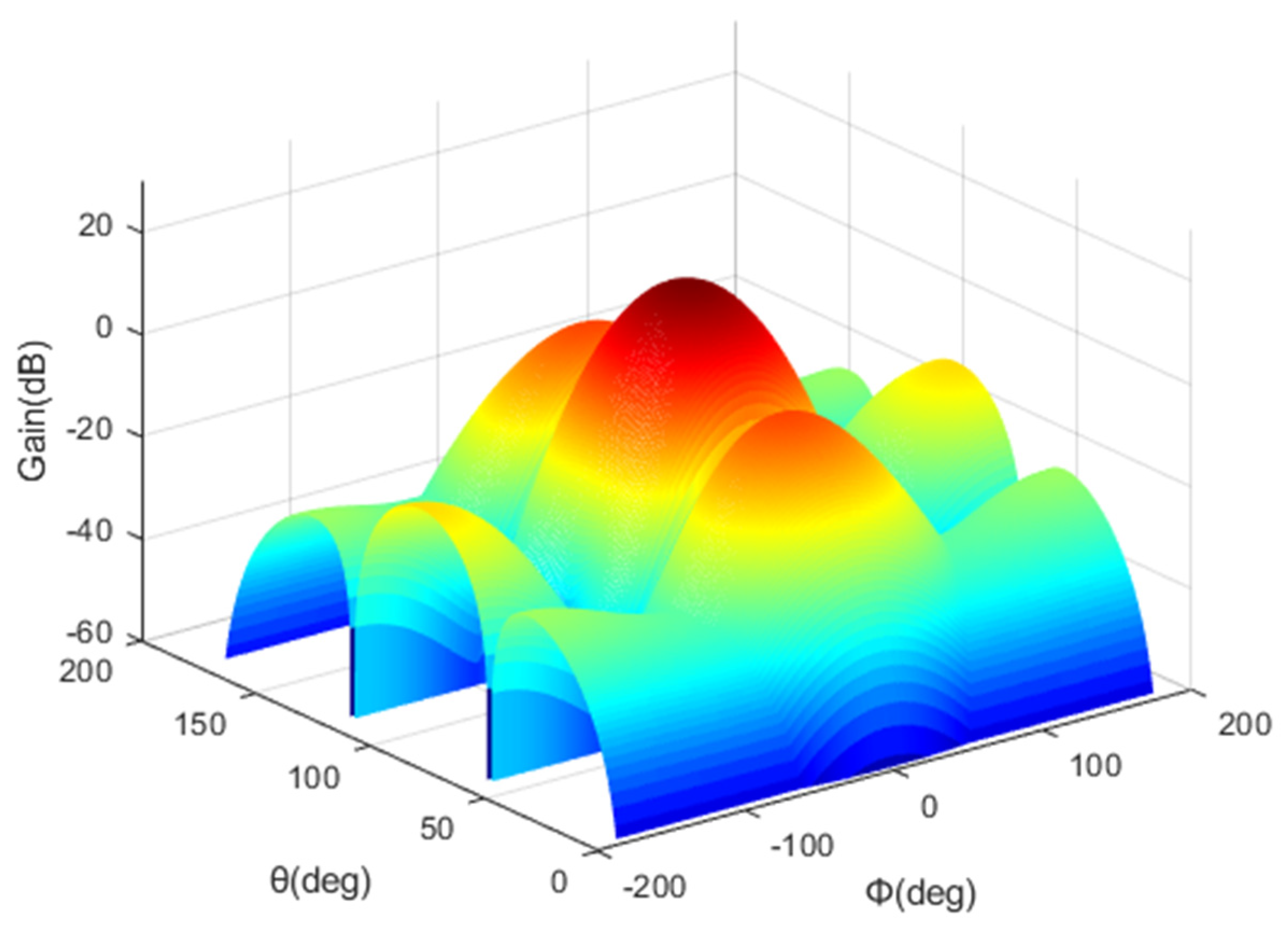
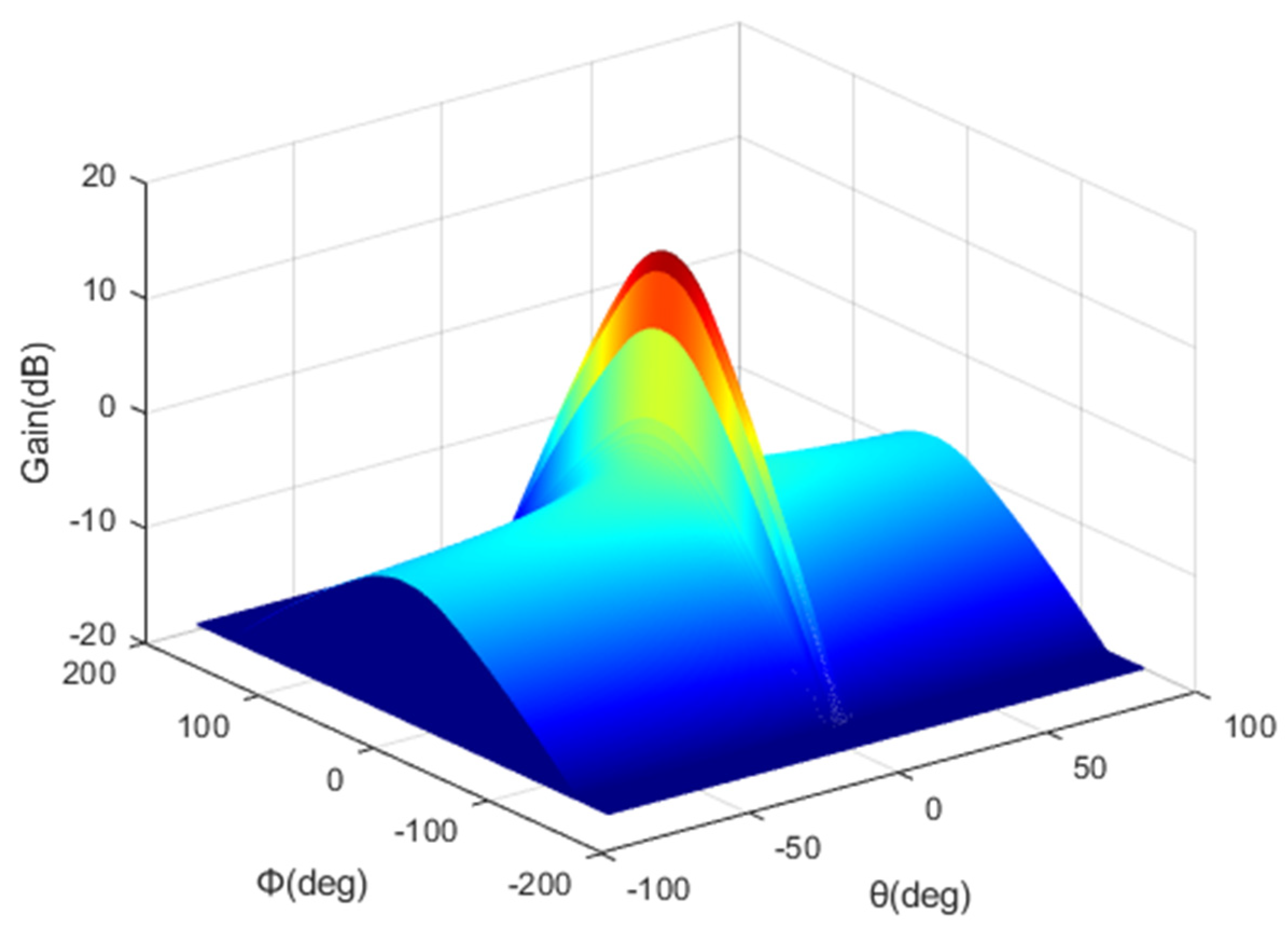
2.2. HAPS Model
2.3. Interfered System Model
2.4. Path Loss Model
3. Calculation of Downlink SINR and
3.1. Calculation of Downlink SINR
3.2. Calculation of
4. DQL-Based HAPS Transmission Power Control Algorithm
4.1. Problem Formulation
4.2. Proposed Algorithm
| Algorithm 1. Training Process for the DQL-Based HAPS Power Control Algorithm |
|
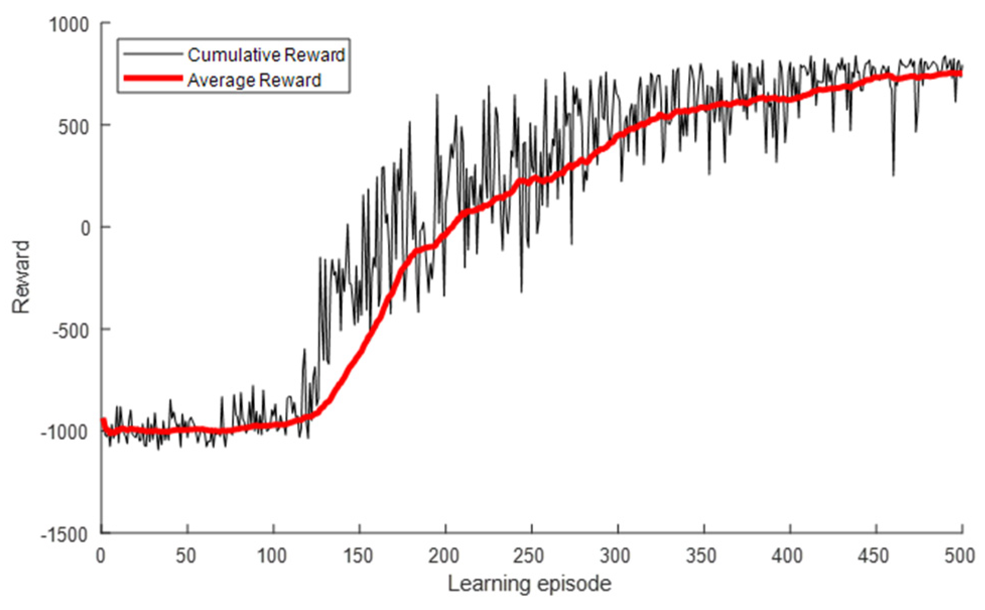
5. Simulation Results
5.1. Simulation Configuration
5.2. Numerical Analysis
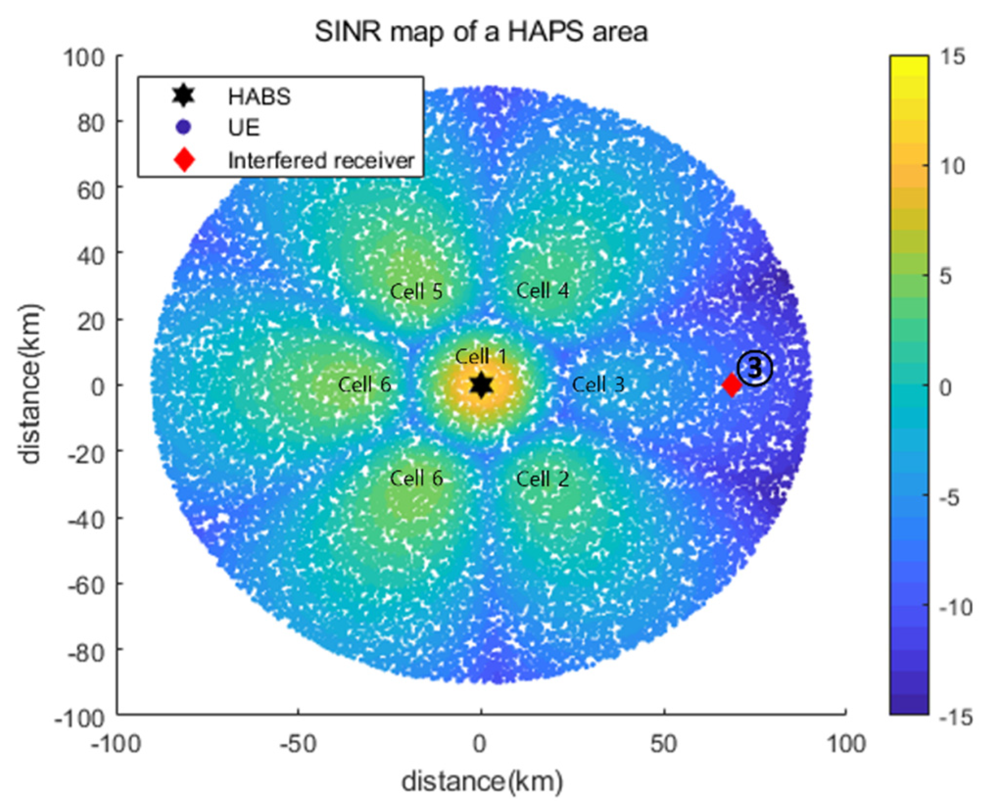
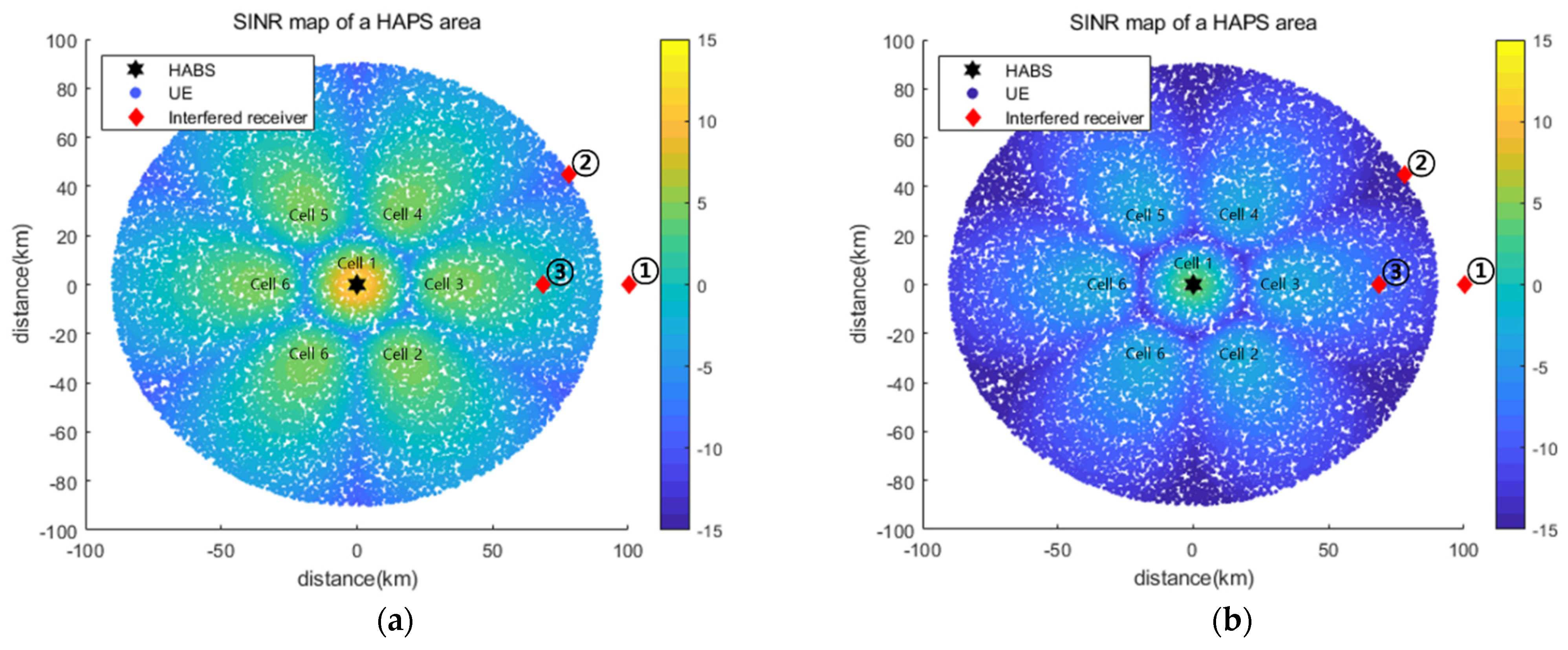
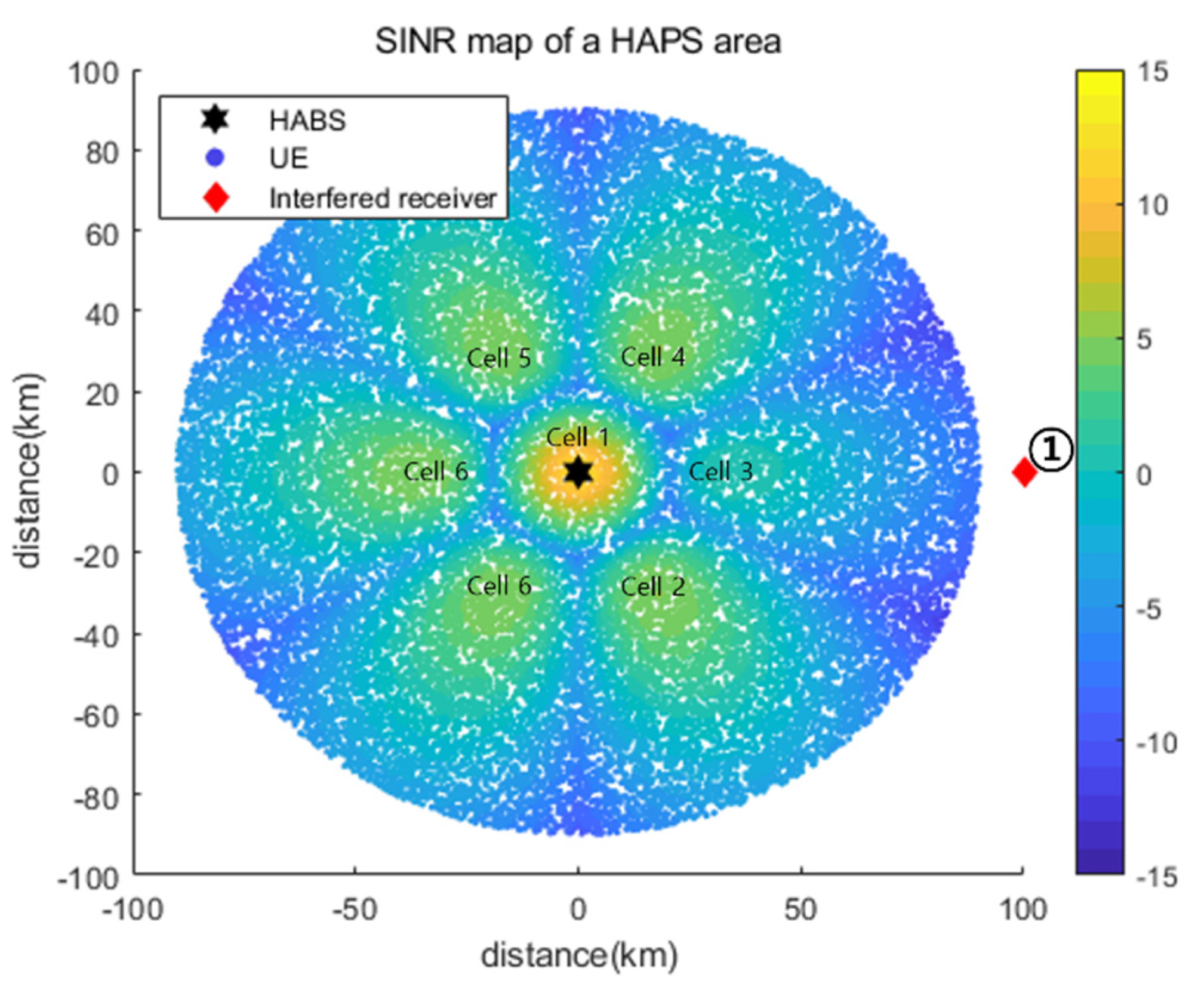
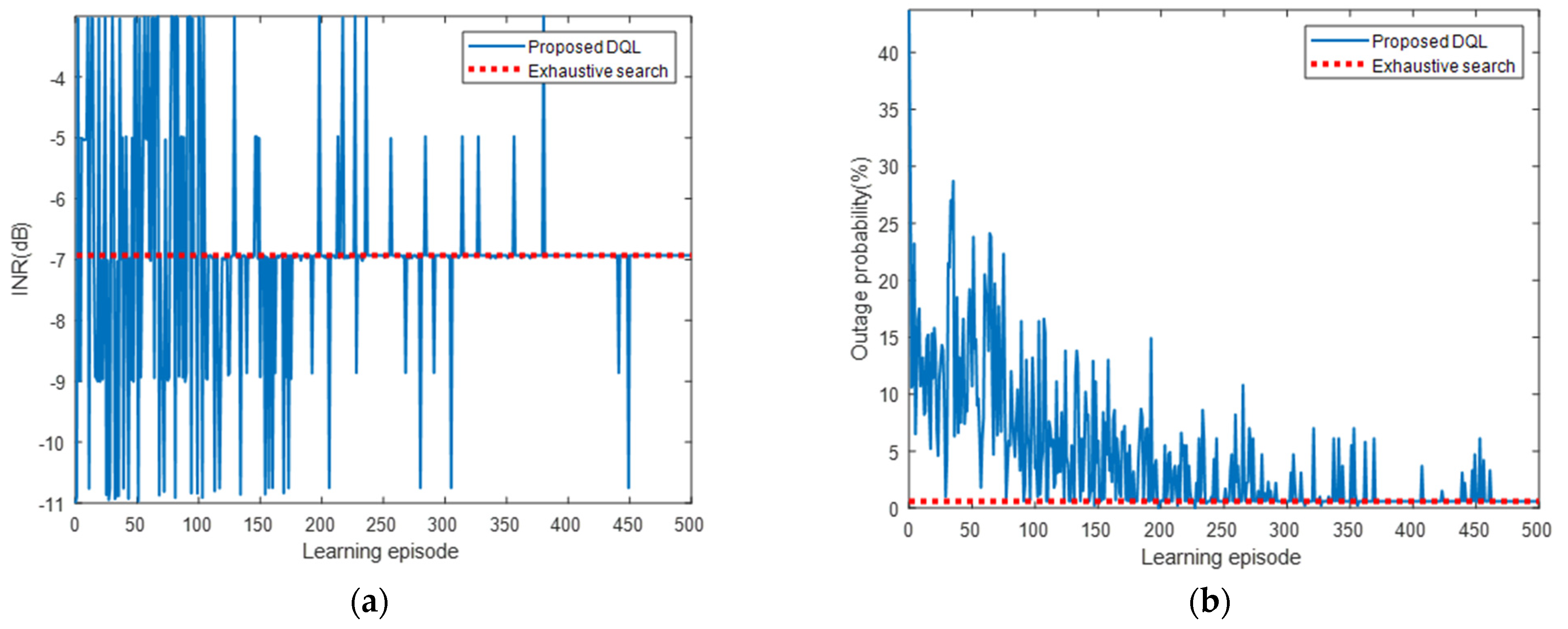
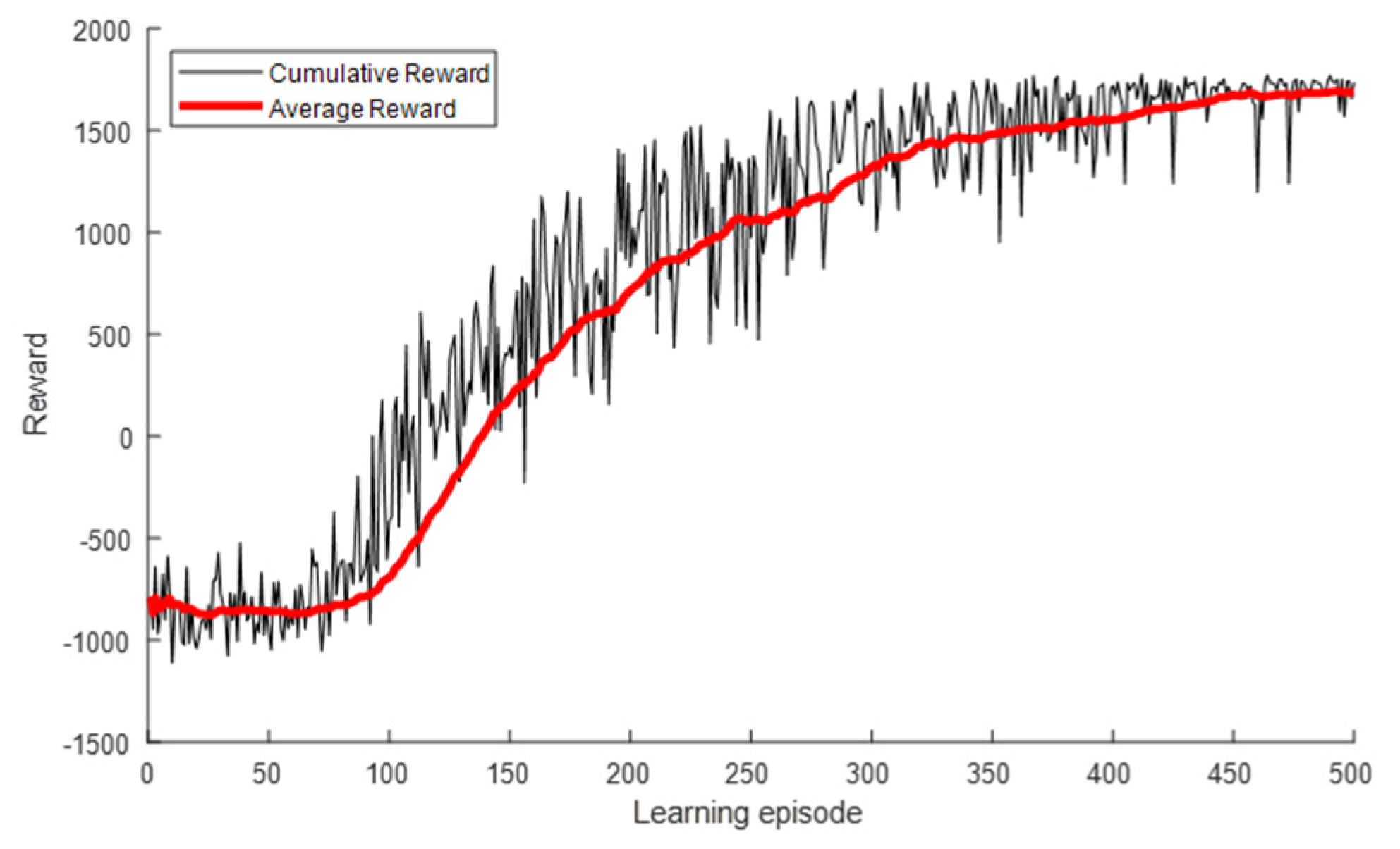
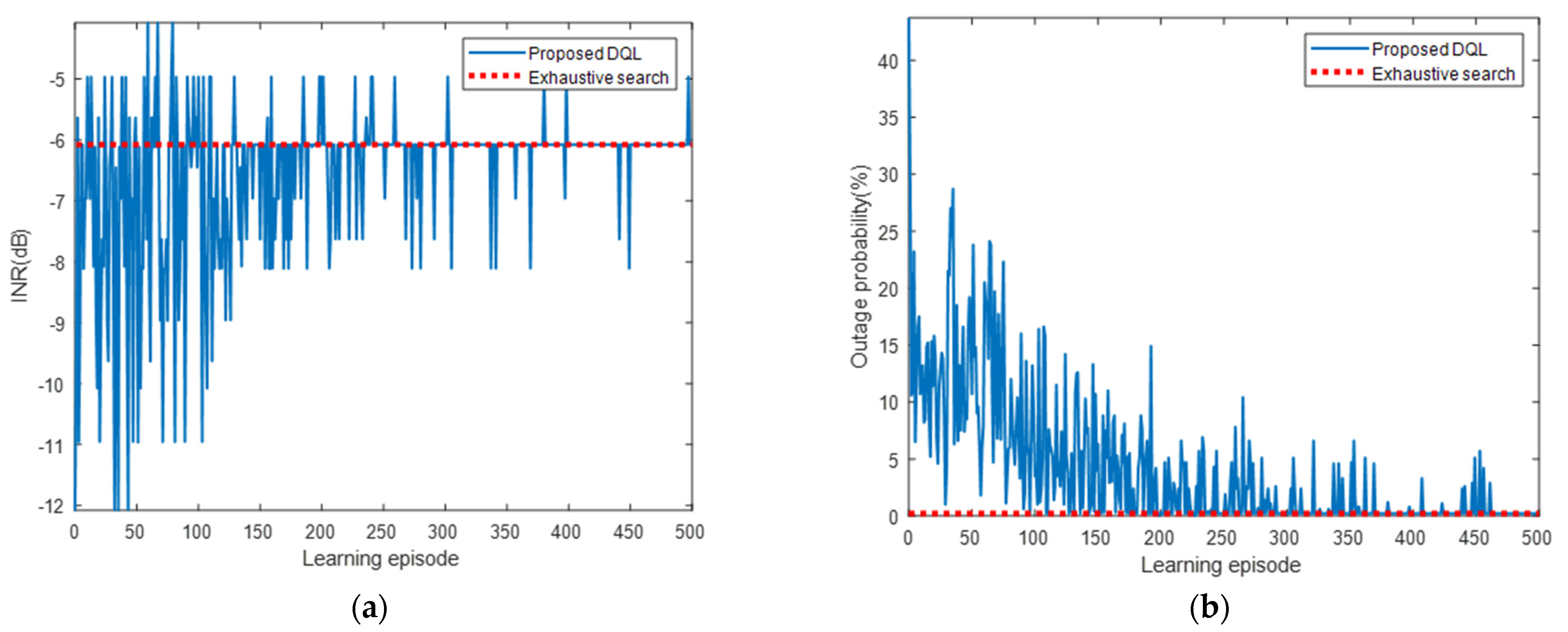
5.2.1. Simulation Results for Interfered Receiver ①
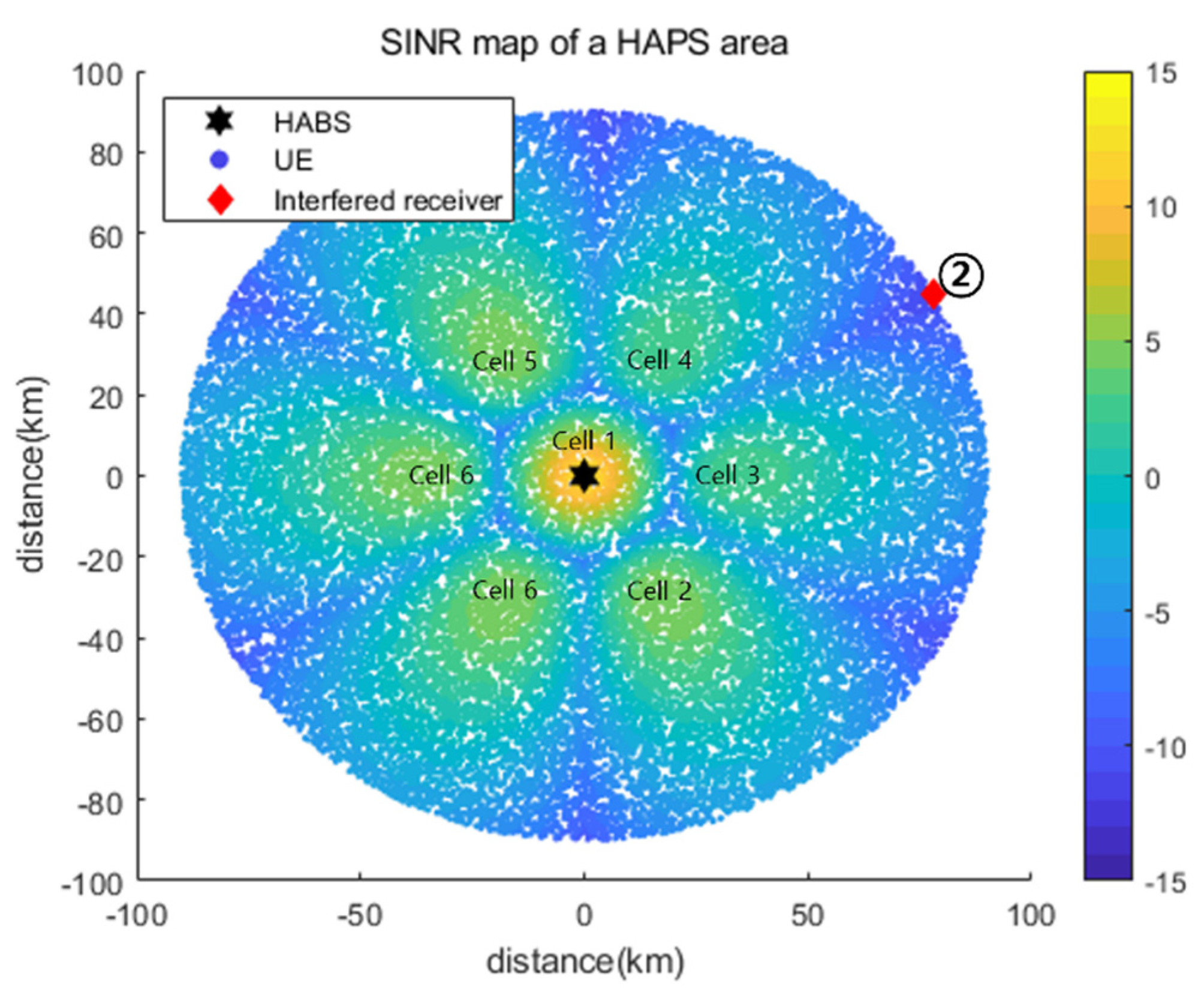
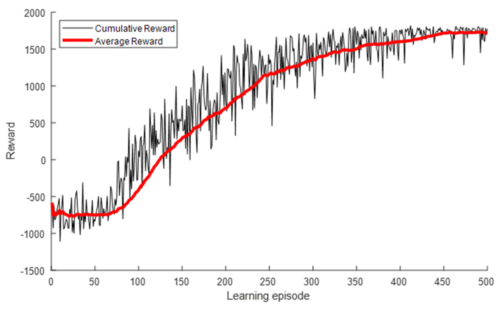
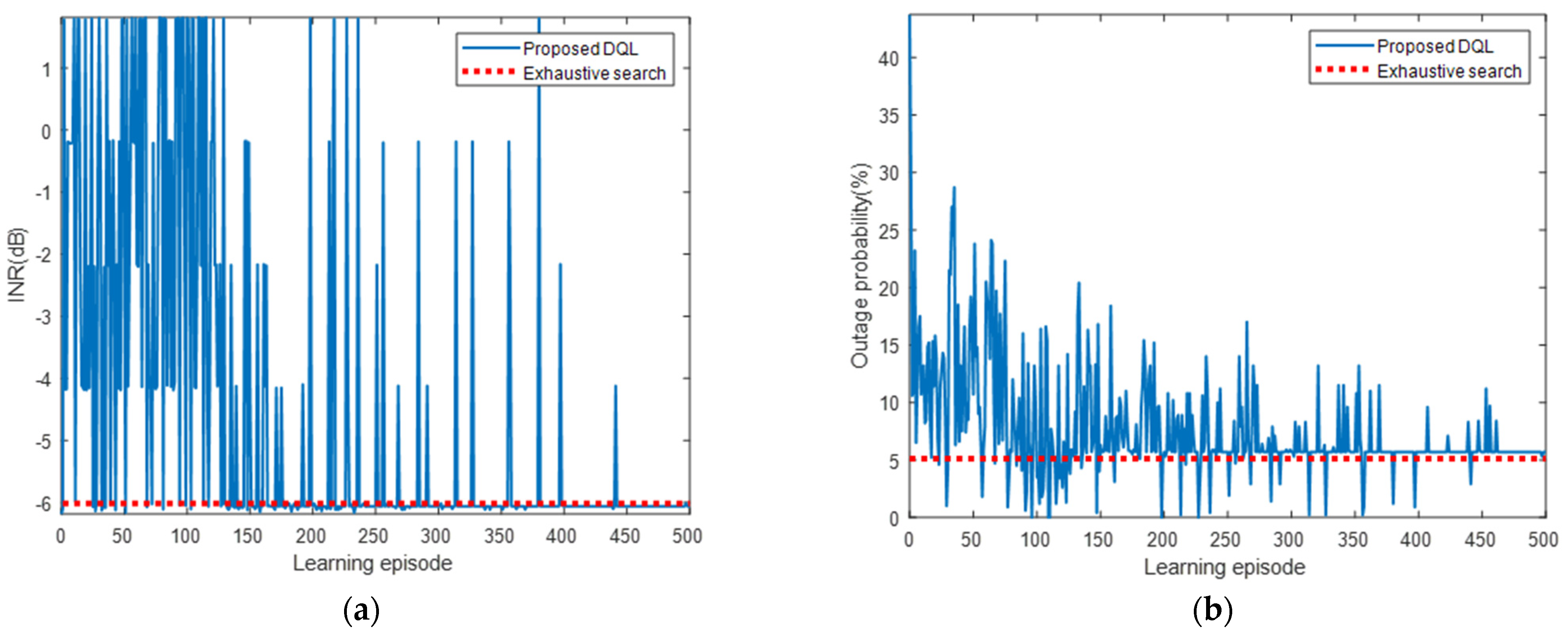
5.2.2. Simulation Results for Interfered Receiver ②
5.2.3. Simulation Results for Interfered Receiver ③
6. Conclusions
Author Contributions
Funding
Institutional Review Board Statement
Informed Consent Statement
Data Availability Statement
Conflicts of Interest
References
- Arum, S.C.; Grace, D.; Mitchell, P.D. A review of wireless communication using high-altitude platforms for extended coverage and capacity. Comput. Commun. 2020, 157, 232–256. [Google Scholar] [CrossRef]
- Alam, M.S.; Kurt, G.K.; Yanikomeroglu, H.; Zhu, P.; Đào, N.D. High altitude platform station based super macro base station constellations. IEEE Commun. Mag. 2021, 59, 103–109. [Google Scholar] [CrossRef]
- Kurt, G.K.; Khoshkholgh, M.G.; Alfattani, S.; Ibrahim, A.; Darwish, T.S.; Alam, M.S.; Yanikomeroglu, H.; Yongacoglu, A. A vision and framework for the high altitude platform station (HAPS) networks of the future. IEEE Commun. Surv. Tutor. 2021, 23, 729–779. [Google Scholar] [CrossRef]
- Hsieh, F.; Jardel, F.; Visotsky, E.; Vook, F.; Ghosh, A.; Picha, B. UAV-based Multi-cell HAPS Communication: System Design and Performance Evaluation. In Proceedings of the GLOBECOM 2020-2020 IEEE Global Communications Conference, Taipei, Taiwan, 7–11 December 2020. [Google Scholar]
- Xing, Y.; Hsieh, F.; Ghosh, A.; Rappaport, T.S. High Altitude Platform Stations (HAPS): Architecture and System Performance. In Proceedings of the 2021 IEEE 93rd Vehicular Technology Conference (VTC2021-Spring), Online, 7–11 April 2021. [Google Scholar]
- International Telecommunications Union (ITU). World Radio Communication Conference 2019 (WRC-19) Final Acts; International Telecommunications Union: Geneva, Switzerland, 2020; p. 366. [Google Scholar]
- Ibrahim, A.; Alfa, A.S. Using Lagrangian relaxation for radio resource allocation in high altitude platforms. IEEE Trans. Wirel. Commun. 2015, 14, 5823–5835. [Google Scholar] [CrossRef] [Green Version]
- Guan, M.; Wu, Z.; Cui, Y.; Cao, X.; Wang, L.; Ye, J.; Peng, B. An intelligent wireless channel allocation in HAPS 5G communication system based on reinforcement learning. EURASIP J. Wirel. Commun. Netw. 2019, 2019, 1–9. [Google Scholar] [CrossRef] [Green Version]
- Guan, M.; Wang, L.; Chen, L. Channel allocation for hot spot areas in HAPS communication based on the prediction of mobile user characteristics. Intell. Autom. Soft Comput. 2016, 22, 613–620. [Google Scholar] [CrossRef]
- Oodo, M.; Miura, R.; Hori, T.; Morisaki, T.; Kashiki, K.; Suzuki, M. Sharing and compatibility study between fixed service using high altitude platform stations (HAPS) and other services in the 31/28 GHz bands. Wirel. Pers. Commun. 2002, 23, 3–14. [Google Scholar] [CrossRef]
- Mokayef, M.; Rahman, T.A.; Ngah, R.; Ahmed, M.Y. Spectrum sharing model for coexistence between high altitude platform system and fixed services at 5.8 GHz. Int. J. Multimed. Ubiquitous Eng. 2013, 8, 265–275. [Google Scholar] [CrossRef]
- Lee, W.; Jeon, Y.; Kim, T.; Kim, Y.I. Deep Reinforcement Learning for UAV Trajectory Design Considering Mobile Ground Users. Sensors 2021, 21, 8239. [Google Scholar] [CrossRef] [PubMed]
- Koushik, A.M.; Hu, F.; Kumar, S. Deep Q-Learning-Based Node Positioning for Throughput-Optimal Communications in Dynamic UAV Swarm Network. IEEE Trans. Cogn. Commun. Netw. 2019, 5, 554–566. [Google Scholar] [CrossRef]
- Raja, G.; Anbalagan, S.; Narayanan, V.S.; Jayaram, S.; Ganapathisubramaniyan, A. Inter-UAV collision avoidance using Deep-Q-learning in flocking environment. In Proceedings of the 2019 IEEE 10th Annual Ubiquitous Computing, Electronics and Mobile Communication Conference, New York, NY, USA, 10–12 October 2019; pp. 1089–1095. [Google Scholar]
- Fotouhi, A.; Ding, M.; Hassan, M. Deep Q-Learning for Two-Hop Communications of Drone Base Stations. Sensors 2021, 21, 1960. [Google Scholar] [CrossRef] [PubMed]
- Anicho, O.; Charlesworth, P.B.; Baicher, G.S.; Nagar, A.K. Reinforcement learning versus swarm intelligence for autonomous multi-HAPS coordination. SN Appl. Sci. 2021, 3, 1–11. [Google Scholar] [CrossRef]
- Hasselt, H.V.; Guez, A.; Silver, D. Deep reinforcement learning with double q-learning. In Proceedings of the Thirtieth AAAI Conference on Artificial Intelligence, Phoenix, AZ, USA, 12–17 February 2016. [Google Scholar]
- International Telecommunications Union Radiocommunication Sector (ITU-R). Working Document towards a Preliminary Draft New Report ITU-R M.[HIBS-CHARACTERISTICS]/Working Document Related to WRC-23 Agenda Item 1.4; R19-WP5D Contribution 716 (Chapter 4-Annex 4.19); International Telecommunications Union: Geneva, Switzerland, 2021. [Google Scholar]
- International Telecommunications Union Radiocommunication Sector (ITU-R). Modelling and Simulation of IMT Networks and Systems for Use in Sharing and Compatibility Studies; Recommendation ITU-R M.2101-0; International Telecommunications Union: Geneva, Switzerland, 2017. [Google Scholar]
- International Telecommunications Union Radiocommunication Sector (ITU-R). Reference Radiation Patterns of Omnidirectional, Sectoral and Other Antennas for the Fixed and Mobile Service for Use in Sharing Studies in the Frequency Range from 400 MHz to about 70 GHz; Recommendation ITU-R F.1336-5; International Telecommunications Union: Geneva, Switzerland, 2019. [Google Scholar]
- International Telecommunications Union Radiocommunication Sector (ITU-R). Propagation Data Required for the Evaluation of Interference between Stations in Space and Those on the Surface of the Earth; Recommendation ITU-R P.619-5; International Telecommunications Union: Geneva, Switzerland, 2021. [Google Scholar]
- International Telecommunications Union Radiocommunication Sector (ITU-R). Working Document towards Sharing and Compatibility Studies of HIBS under WRC-23 Agenda Item 1.4—Sharing and Compatibility Studies of High-Altitude Platform Stations as IMT Base Stations (HIBS) on WRC-23 Agenda Item 1.4; R19-WP5D Contribution 716 (Chapter 4—Annex 4.20); International Telecommunications Union: Geneva, Switzerland, 2021. [Google Scholar]
- Mnih, V.; Kavucuoglu, K.; Silver, D.; Rusu, A.A.; Veness, J.; Bellemare, M.G.; Graves, A.; Riedmiller, M.; Fidjeland, A.K.; Ostrovski, G.; et al. Human-level control through deep reinforcement learning. Nature 2015, 518, 529–533. [Google Scholar] [CrossRef] [PubMed]
- International Telecommunications Union Radiocommunication Sector (ITU-R). Characteristics of Terrestrial Component of IMT for Sharing and Compatibility Studies in Preparation for WRC-23; R19-WP5D Temporary Document 422 (Revision 2); International Telecommunications Union: Geneva, Switzerland, 2021. [Google Scholar]


| Parameter | Value |
|---|---|
| 2545 MHz | |
| ) | 20 MHz |
| Area radius | 90 km |
| ) | 20 km |
| ) | 7 |
| Antenna pattern | Recommendation ITU-R M.2101 |
| ) | 8 dBi |
| Horizontal/vertical 3 dB beamwidth of single element | 65° for both H/V |
| Antenna array configuration (Row × column) | 2 × 2 elements (1st layer cell) 4 × 2 elements (2nd layer cell) |
| 2 dB | |
| Antenna tilt | 90° (1st layer cell) 23° (2nd layer cell) |
| Antenna polarization | Linear/±45° |
| ) | 1000 |
| UE height | 1.5 m |
| UE antenna gain | −3 dBi |
| ) | −10 dB |
| Parameter | Value |
|---|---|
| 2545 MHz | |
| ) | 20 MHz |
| 5 dB | |
| 20 m | |
| Antenna tilt | 10° |
| Antenna pattern | Recommendation ITU-R F.1336 (recommends 3.1) Horizontal 3 dB beamwidth: 65° Vertical 3 dB beamwidth is determined from the horizontal beamwidth equations in Recommendation ITU-R F.1336. Vertical beam widths of actual antennas may also be used when available. |
| Antenna polarization | Linear/±45° |
| 16 dBi | |
| ) | −6 dB |
| Interfered Receiver | Location (km) | ||||
|---|---|---|---|---|---|
| ① | 100, 0, 0.02 | −3.01 | −11.01 | 0 | 43.7 |
| ② | 77.9, 45, 0.02 | −4.08 | −12.08 | 0 | 43.7 |
| ③ | 65.8, 0, 0.02 | 1.81 | −6.19 | 0 | 43.7 |
(dB) | (%) | ||||||||
|---|---|---|---|---|---|---|---|---|---|
| Optimal | 37 | 34 | 30 | 34 | 34 | 34 | 34 | –6.93 | 0.6 |
| DQL | 37 | 34 | 30 | 34 | 34 | 34 | 34 | –6.93 | 0.6 |
| DDQL | 37 | 34 | 30 | 34 | 34 | 34 | 34 | -6.93 | 0.6 |
| (dBm) | (dBm) | (dBm) | (dB) | (%) | |||||
|---|---|---|---|---|---|---|---|---|---|
| Optimal | 37 | 34 | 32 | 32 | 34 | 34 | 34 | −6.08 | 0.2 |
| DQL | 37 | 34 | 32 | 32 | 34 | 34 | 34 | −6.08 | 0.2 |
| DDQL | 37 | 34 | 32 | 32 | 34 | 34 | 34 | −6.08 | 0.2 |
| (dBm) | (dBm) | (dBm) | (dB) | (%) | |||||
|---|---|---|---|---|---|---|---|---|---|
| Optimal | 37 | 34 | 26 | 32 | 34 | 34 | 34 | −6.02 | 5.1 |
| DQL | 37 | 32 | 26 | 32 | 34 | 34 | 34 | −6.06 | 5.7 |
| DDQL | 37 | 32 | 26 | 32 | 34 | 34 | 34 | −6.06 | 5.7 |
Publisher’s Note: MDPI stays neutral with regard to jurisdictional claims in published maps and institutional affiliations. |
© 2022 by the authors. Licensee MDPI, Basel, Switzerland. This article is an open access article distributed under the terms and conditions of the Creative Commons Attribution (CC BY) license (https://creativecommons.org/licenses/by/4.0/).
Share and Cite
Jo, S.; Yang, W.; Choi, H.K.; Noh, E.; Jo, H.-S.; Park, J. Deep Q-Learning-Based Transmission Power Control of a High Altitude Platform Station with Spectrum Sharing. Sensors 2022, 22, 1630. https://doi.org/10.3390/s22041630
Jo S, Yang W, Choi HK, Noh E, Jo H-S, Park J. Deep Q-Learning-Based Transmission Power Control of a High Altitude Platform Station with Spectrum Sharing. Sensors. 2022; 22(4):1630. https://doi.org/10.3390/s22041630
Chicago/Turabian StyleJo, Seongjun, Wooyeol Yang, Haing Kun Choi, Eonsu Noh, Han-Shin Jo, and Jaedon Park. 2022. "Deep Q-Learning-Based Transmission Power Control of a High Altitude Platform Station with Spectrum Sharing" Sensors 22, no. 4: 1630. https://doi.org/10.3390/s22041630
APA StyleJo, S., Yang, W., Choi, H. K., Noh, E., Jo, H.-S., & Park, J. (2022). Deep Q-Learning-Based Transmission Power Control of a High Altitude Platform Station with Spectrum Sharing. Sensors, 22(4), 1630. https://doi.org/10.3390/s22041630