
On the Design of a Thermo-Magnetically Activated Piezoelectric Micro-Energy Generator: Working Principle


Abstract
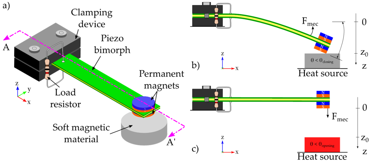
:1. Introduction
2. Materials and Methods
3. Analytical Modeling
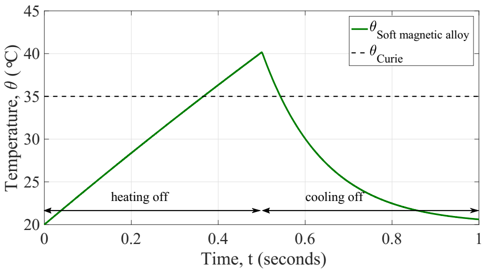
3.1. Heat Transfer Model
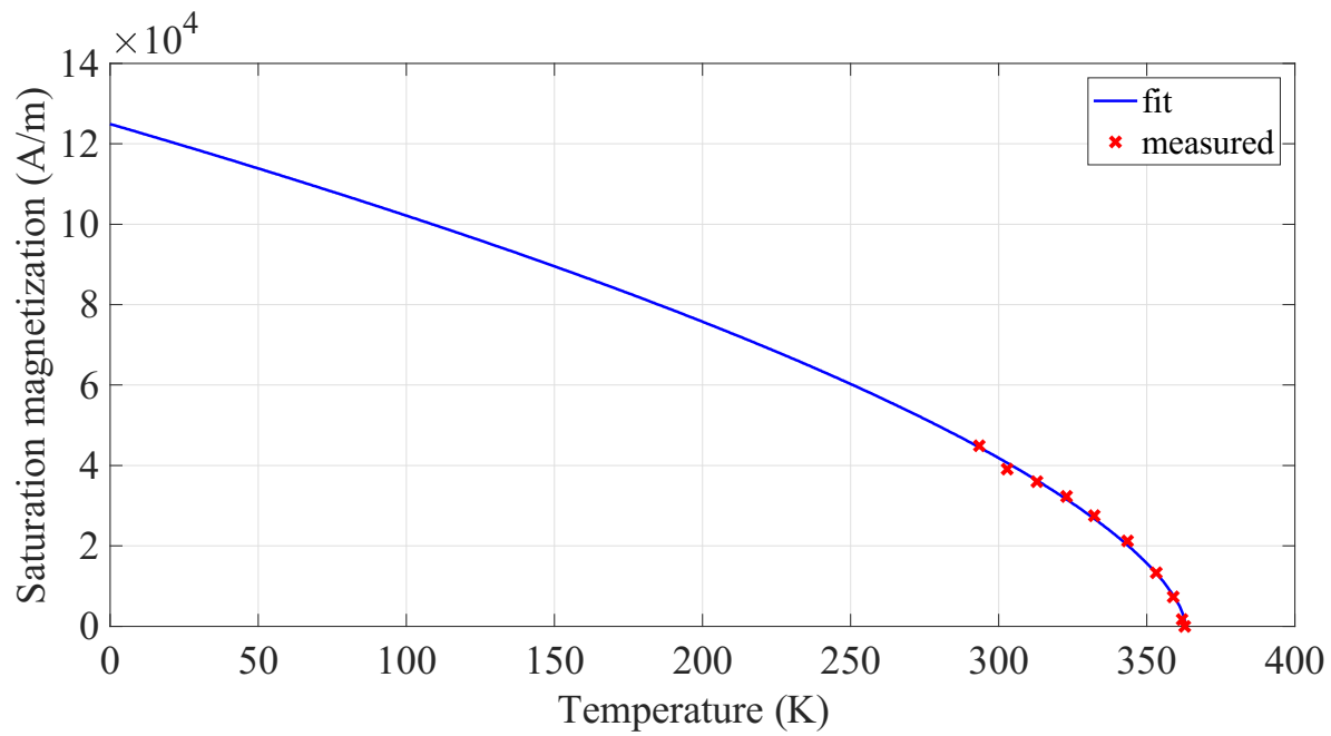
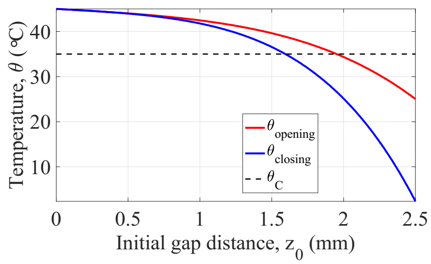
3.2. Thermo-Magnetic Model
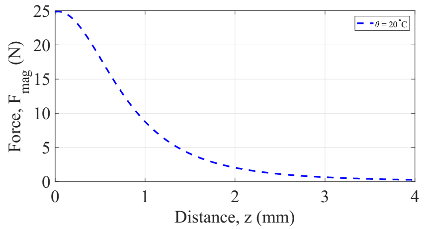
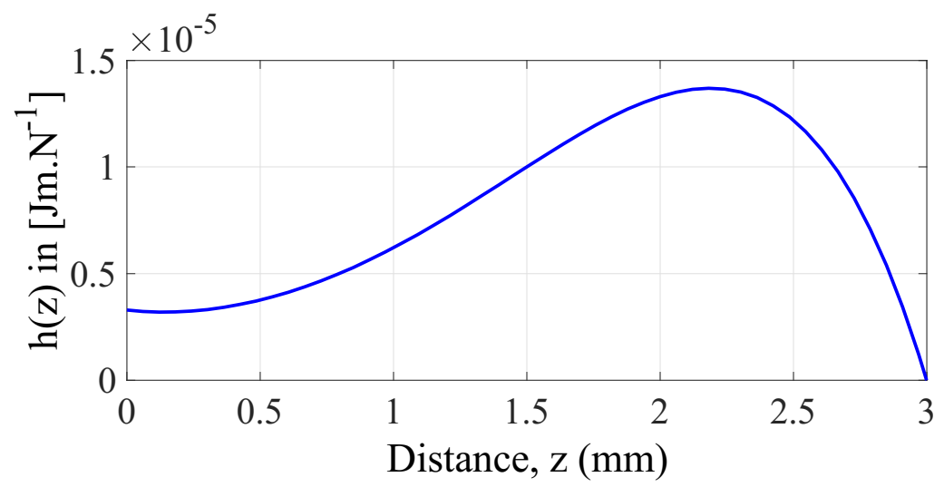
3.3. Magnetic Force
3.4. Vibration Model
3.5. Global Coupling Model
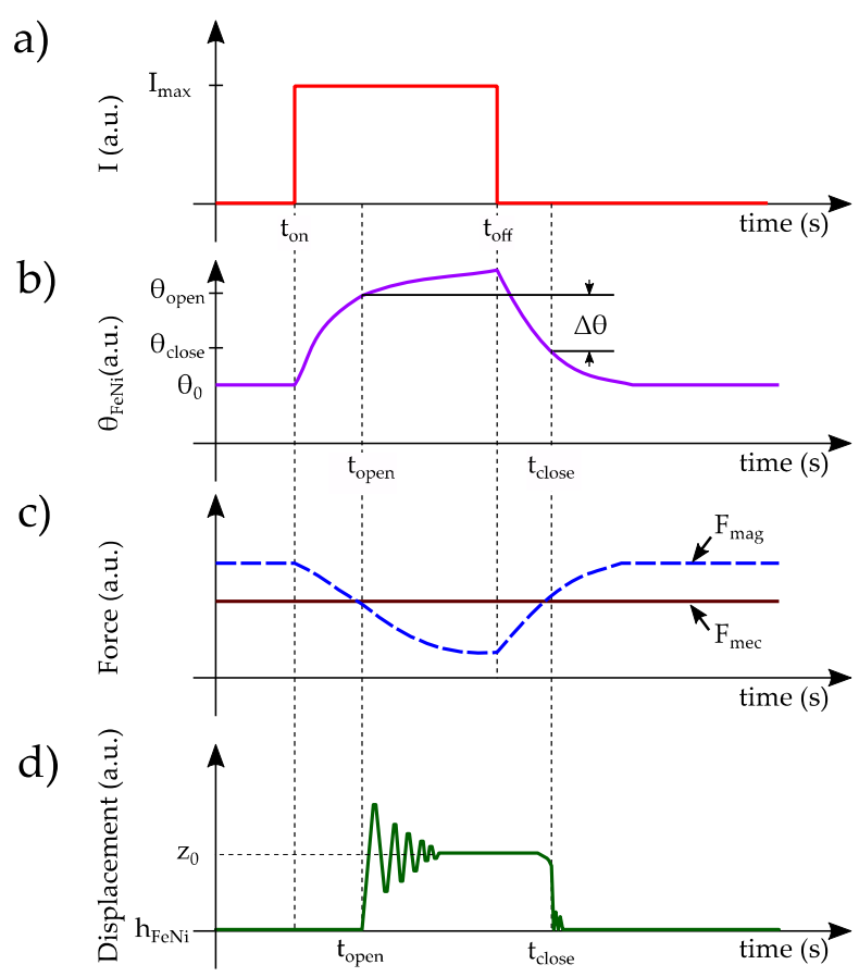
4. Results and Discussion
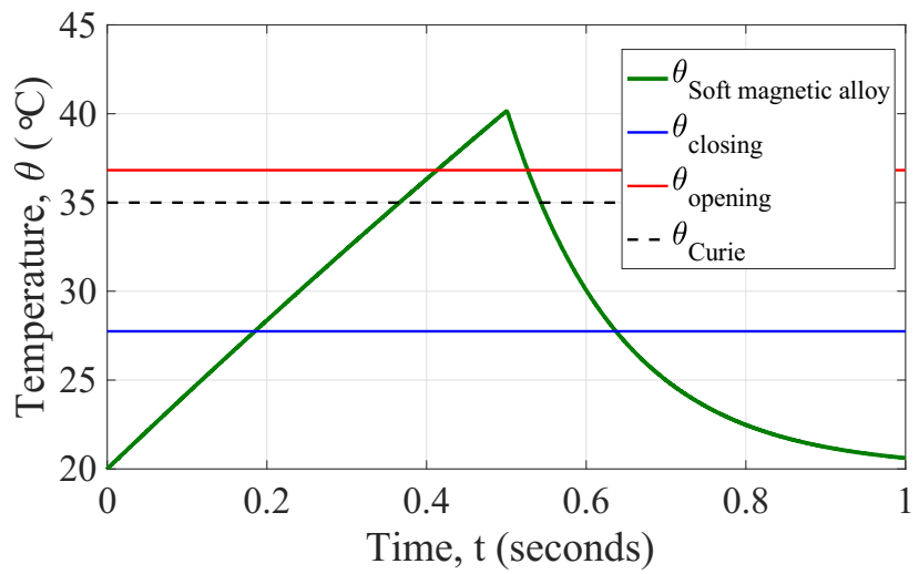
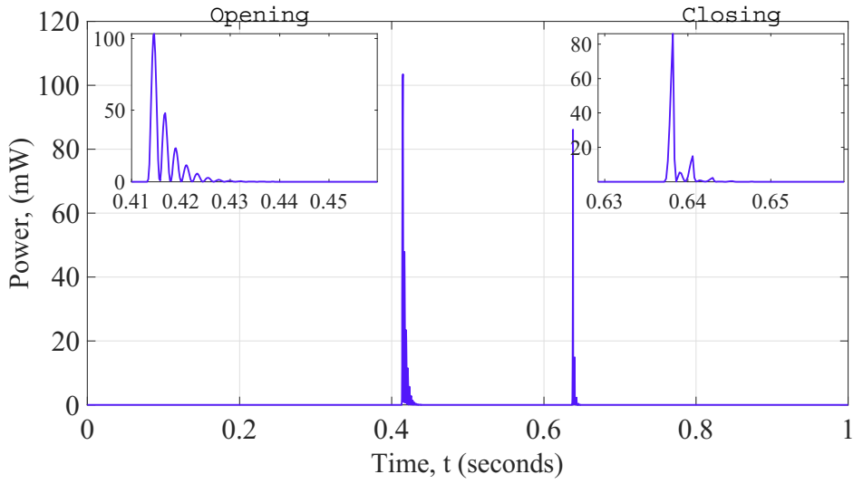
Generator Dynamic Behavior
5. Conclusions
Author Contributions
Funding
Institutional Review Board Statement
Informed Consent Statement
Data Availability Statement
Conflicts of Interest
References
- Li, H.; Tian, C.; Deng, Z.D. Energy Harvesting from Low Frequency Applications Using Piezoelectric Materials. Appl. Phys. Rev. 2014, 1, 041301. [Google Scholar] [CrossRef] [Green Version]
- Kim, H.S.; Kim, J.-H.; Kim, J. A Review of Piezoelectric Energy Harvesting Based on Vibration. Int. J. Precis. Eng. Manuf. 2011, 12, 1129–1141. [Google Scholar] [CrossRef]
- Anton, S.R.; Sodano, H.A. A Review of Power Harvesting Using Piezoelectric Materials (2003–2006). Smart Mater. Struct. 2007, 16, R1–R21. [Google Scholar] [CrossRef]
- Fu, H.; Mei, X.; Yurchenko, D.; Zhou, S.; Theodossiades, S.; Nakano, K.; Yeatman, E.M. Rotational Energy Harvesting for Self-Powered Sensing. Joule 2021, 5, 1074–1118. [Google Scholar] [CrossRef]
- Su, W.-J.; Lin, J.-H.; Li, W.-C. Analysis of a Cantilevered Piezoelectric Energy Harvester in Different Orientations for Rotational Motion. Sensors 2020, 20, 1206. [Google Scholar] [CrossRef] [PubMed] [Green Version]
- Farhangdoust, S.; Georgeson, G.; Ihn, J.-B.; Chang, F.-K. Kirigami Auxetic Structure for High Efficiency Power Harvesting in Self-Powered and Wireless Structural Health Monitoring Systems. Smart Mater. Struct. 2021, 30, 015037. [Google Scholar] [CrossRef]
- Zou, D.; Liu, S.; Zhang, C.; Hong, Y.; Zhang, G.; Yang, Z. Flexible and Translucent PZT Films Enhanced by the Compositionally Graded Heterostructure for Human Body Monitoring. Nano Energy 2021, 85, 105984. [Google Scholar] [CrossRef]
- Wang, Y.; Yang, Z.; Li, P.; Cao, D.; Huang, W.; Inman, D.J. Energy Harvesting for Jet Engine Monitoring. Nano Energy 2020, 75, 104853. [Google Scholar] [CrossRef]
- Jiang, X.-Y.; Zou, H.-X.; Zhang, W.-M. Design and Analysis of a Multi-Step Piezoelectric Energy Harvester Using Buckled Beam Driven by Magnetic Excitation. Energy Convers. Manag. 2017, 145, 129–137. [Google Scholar] [CrossRef]
- Sothmann, B.; Sánchez, R.; Jordan, A.N. Thermoelectric Energy Harvesting with Quantum Dots. Nanotechnology 2015, 26, 032001. [Google Scholar] [CrossRef] [PubMed] [Green Version]
- Yang, M.-Z.; Wu, C.-C.; Dai, C.-L.; Tsai, W.-J. Energy Harvesting Thermoelectric Generators Manufactured Using the Complementary Metal Oxide Semiconductor Process. Sensors 2013, 13, 2359–2367. [Google Scholar] [CrossRef] [PubMed] [Green Version]
- Prijic, A.; Vracar, L.; Vuckovic, D.; Milic, D.; Prijic, Z. Thermal Energy Harvesting Wireless Sensor Node in Aluminum Core PCB Technology. IEEE Sens. J. 2015, 15, 337–345. [Google Scholar] [CrossRef]
- Cuadras, A.; Gasulla, M.; Ferrari, V. Thermal Energy Harvesting through Pyroelectricity. Sens. Actuators A Phys. 2010, 158, 132–139. [Google Scholar] [CrossRef]
- Chang, H.H.S.; Huang, Z. Laminate Composites with Enhanced Pyroelectric Effects for Energy Harvesting. Smart Mater. Struct. 2010, 19, 065018. [Google Scholar] [CrossRef]
- Sandoval, S.M.; Sepulveda, A.E.; Keller, S.M. On the Thermodynamic Efficiency of a Nickel-Based Multiferroic Thermomagnetic Generator: From Bulk to Atomic Scale. J. Appl. Phys. 2015, 117, 163920. [Google Scholar] [CrossRef]
- Smoker, J.; Nouh, M.; Aldraihem, O.; Baz, A. Energy Harvesting from a Standing Wave Thermoacoustic-Piezoelectric Resonator. J. Appl. Phys. 2012, 111, 104901. [Google Scholar] [CrossRef]
- Babaei, H.; Siddiqui, K. Design and Optimization of Thermoacoustic Devices. Energy Convers. Manag. 2008, 49, 3585–3598. [Google Scholar] [CrossRef]
- Furlani, E.P. Permanent Magnet and Electromechanical Devices. In Electromagnetism; Elsevier: Amsterdam, The Netherlands, 2001. [Google Scholar] [CrossRef]
- Raghunathan, A.; Melikhov, Y.; Snyder, J.E.; Jiles, D.C. Theoretical Model of Temperature Dependence of Hysteresis Based on Mean Field Theory. IEEE Trans. Magn. 2010, 46, 1507–1510. [Google Scholar] [CrossRef]
- Mavrudieva, D.; Voyant, J.-Y.; Kedous-Lebouc, A.; Yonnet, J.-P. Magnetic Structures for Contactless Temperature Sensor. Sens. Actuators A Phys. 2008, 142, 464–467. [Google Scholar] [CrossRef]
- MEMS: A Practical Guide to Design, Analysis, and Applications; Korvink, J.G.; Paul, O. (Eds.) Springer: Berlin/Heidelberg, Germany, 2006; ISBN 978-3-540-21117-4. [Google Scholar]
- Badel, A. Récupération d’énergie et contrôle vibratoire par éléments piézoélectriques suivant une approche non linéaire. Ph.D. Dissertation, Université de Savoie, Chambéry, France, 2005. [Google Scholar]


| Parameter | Symbol | Units | Value |
|---|---|---|---|
| Surface area of device | |||
| Surface area of soft magnetic alloy | |||
| Mass | |||
| Specific heat | 505 | ||
| Electrical current | 2 | ||
| Electrical resistance | 20 | ||
| Heat transfer coefficient | 28 | ||
| Fan speed | 2000 | ||
| Mass flow rate |
| Parameter | Symbol | Units | Value |
|---|---|---|---|
| Saturation magnetization at 0 K | |||
| Critical exponent | - | 0.625 | |
| Curie temperature | 363.15 |
| Parameter | Symbol | Units | Value |
|---|---|---|---|
| Remanent flux density of magnet | |||
| Thickness of magnet | |||
| Radius of magnet | |||
| Permeability of vacuum |
| Parameter | Symbol | Units | Value |
|---|---|---|---|
| Thickness of soft magnetic material | |||
| Radius of soft magnetic material | |||
| Saturation magnetization at 0 K |
| System | Parameter | Symbol | Units | Value |
|---|---|---|---|---|
| Transducer system cantilever beam | Length of cantilever beam | 20 | ||
| Width of cantilever beam | 4 | |||
| Thickness of shim layer | 100 | |||
| Young’s modulus of shim layer | 100 | |||
| Poisson’s ratio of shim layer | - | 0.3 | ||
| Density of shim layer | 7500 | |||
| Transducer system piezoelectric material | Length of piezoelectric layer | 20 | ||
| Thickness of piezoelectric layer | 105 | |||
| Stiffness of electrical field | 20.5 | |||
| −8.45 | ||||
| −4.78 | ||||
| 13.45 | ||||
| Piezoelectric coefficient | −274 | |||
| Permittivity at constant strain | 30.1 | |||
| Permittivity at constant stress | 27.7 | |||
| Triggering system soft magnetic alloy | Radius of soft magnetic alloy | 7.5 | ||
| Thickness of soft magnetic material | 4 | |||
| Density of soft magnetic alloy | 6000 | |||
| Curie temperature | 35 | |||
| Critical exponent | - | 0.625 | ||
| Specific heat of soft magnetic material | 505 | |||
| Saturation magnetization at 0 K | ||||
| Heat transfer coefficient | 28 | |||
| Fan speed | 2000 | |||
| Mass flow rate | 0.5 | |||
| Initial gap distance | 2 | |||
| Triggering system permanent magnet | Radius of magnet | 2 | ||
| Thickness of magnet | 1 | |||
| Density of magnet | 5000 |
| Criterion | Operation | Design Parameter of Impact | Design Rule |
|---|---|---|---|
| Volume of soft magnetic material | Provides thermal dependent magnetization | It has to be strong enough to counter | |
| They have to be as low as possible to reduce the time between commutations | |||
| Volume of magnets | Provides external flux density to induce | An optimal ratio has to be selected to ensure a functional | |
| Acts as seismic mass | It shall be as large as possible to increase natural oscillation | ||
| Volume of piezoelectric transducer | Piezoelectric layers dimensions | An optimal dimension should be considered to maximize the output voltage. As they affect directly the stiffness of the system, thus | |
| Shim layer dimensions | Thickness of layers have greater impact on the system stiffness than the other parameters. | ||
| Changes the surface area of the generator when it is closed | Reducing the lateral surface of the generator can reduce and , thus reduce as well as time between commutations. | ||
| Initial gap distance | Adjusts the operating temperatures and | It has to be as large as possible to increase the stroke of displacement on the cantilever beam, thus higher elastic energy to be converted into electricity | |
| Scales the mechanical restoring force of the transducer beam | By increasing is then increased, which obliges to adjust the magnetic attraction force to get the operation commutation in a feasible range of temperature |
| Energy Density per Commutation | Symbol | Units | Value |
|---|---|---|---|
| Opening commutation | 280 | ||
| Closing commutation | 67 |
Publisher’s Note: MDPI stays neutral with regard to jurisdictional claims in published maps and institutional affiliations. |
© 2022 by the authors. Licensee MDPI, Basel, Switzerland. This article is an open access article distributed under the terms and conditions of the Creative Commons Attribution (CC BY) license (https://creativecommons.org/licenses/by/4.0/).
Share and Cite
Rendon-Hernandez, A.A.; Basrour, S. On the Design of a Thermo-Magnetically Activated Piezoelectric Micro-Energy Generator: Working Principle. Sensors 2022, 22, 1610. https://doi.org/10.3390/s22041610
Rendon-Hernandez AA, Basrour S. On the Design of a Thermo-Magnetically Activated Piezoelectric Micro-Energy Generator: Working Principle. Sensors. 2022; 22(4):1610. https://doi.org/10.3390/s22041610
Chicago/Turabian StyleRendon-Hernandez, Adrian A., and Skandar Basrour. 2022. "On the Design of a Thermo-Magnetically Activated Piezoelectric Micro-Energy Generator: Working Principle" Sensors 22, no. 4: 1610. https://doi.org/10.3390/s22041610
APA StyleRendon-Hernandez, A. A., & Basrour, S. (2022). On the Design of a Thermo-Magnetically Activated Piezoelectric Micro-Energy Generator: Working Principle. Sensors, 22(4), 1610. https://doi.org/10.3390/s22041610