
A Crack Propagation Method for Pipelines with Interacting Corrosion and Crack Defects


Abstract
:1. Introduction
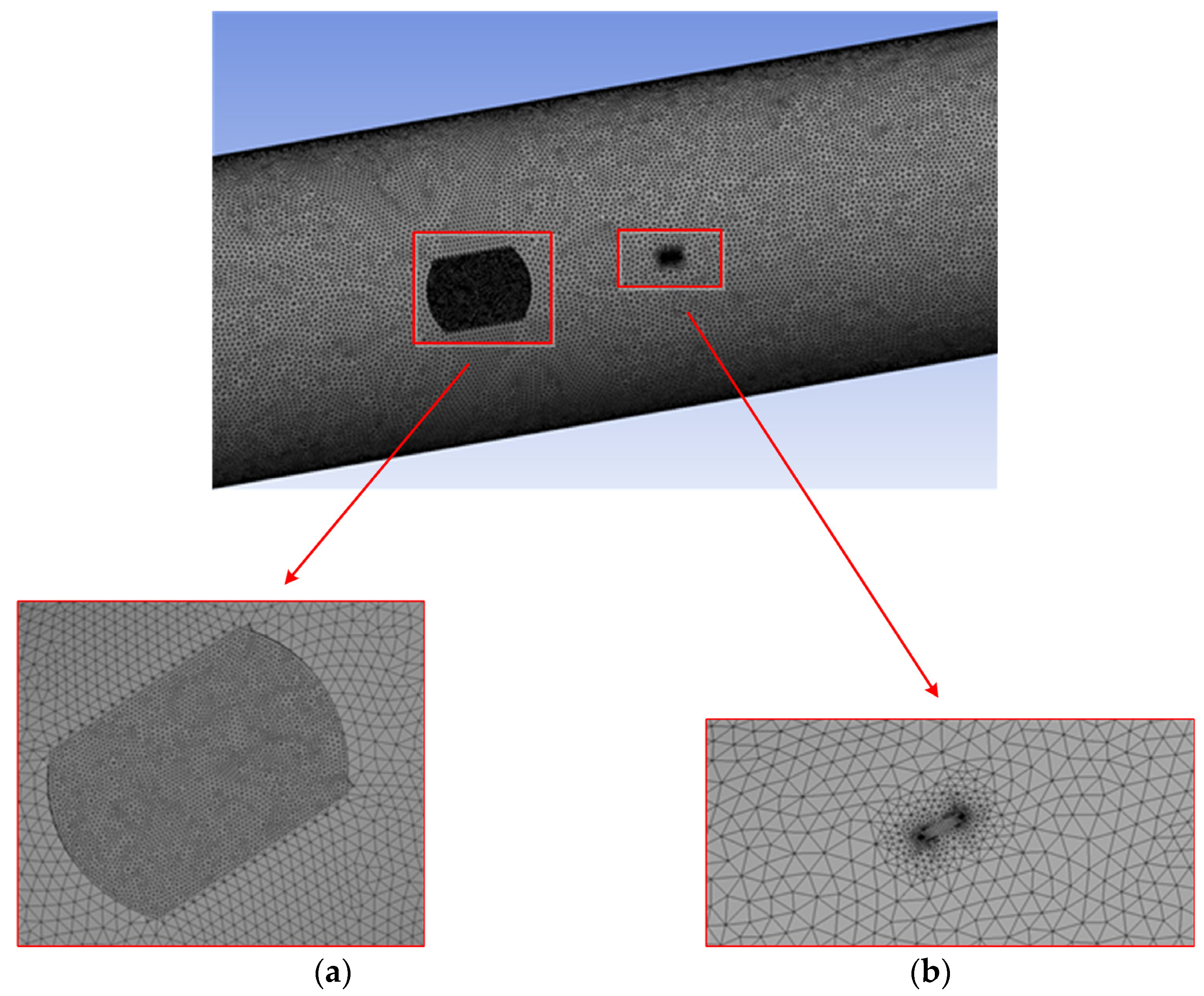
2. The Pipeline Finite Element Analysis Model
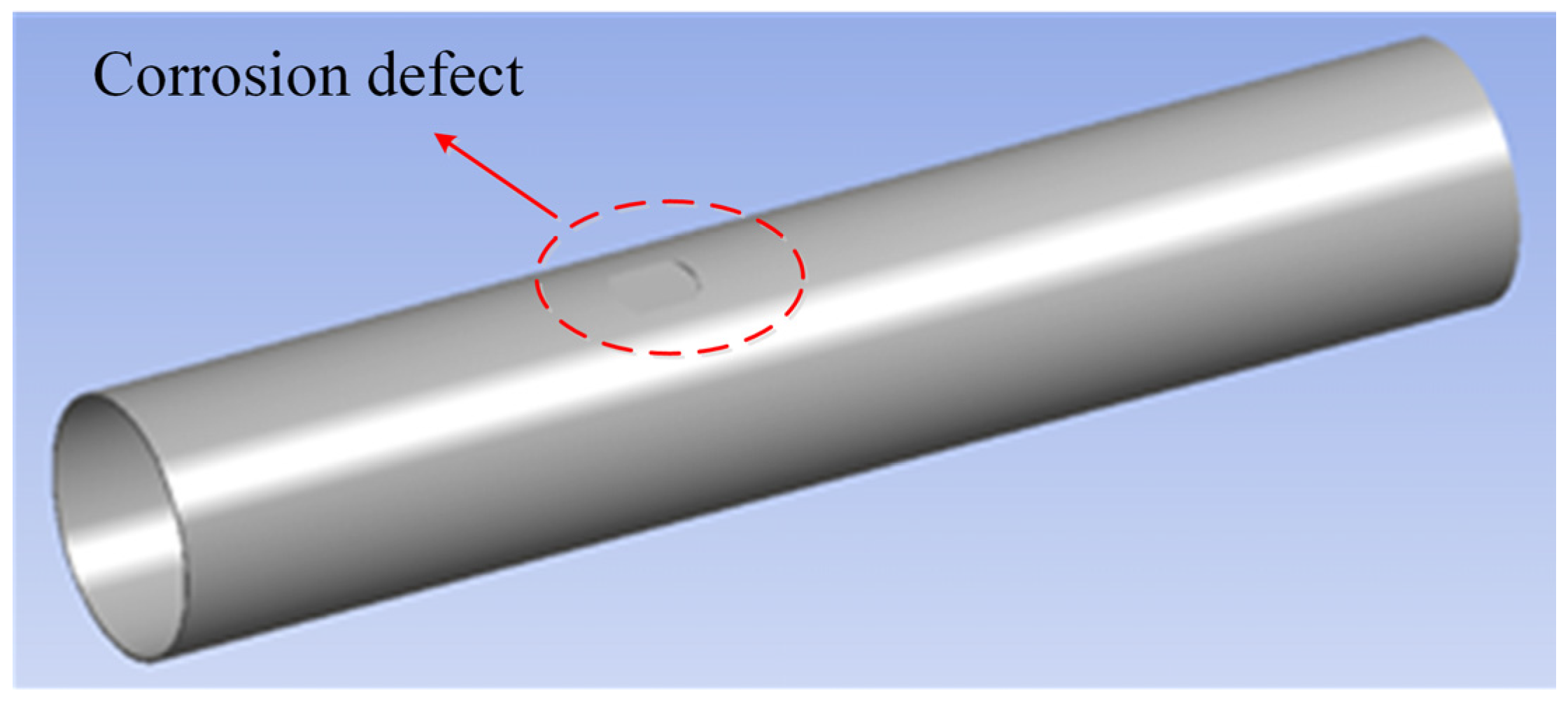
2.1. The FEA Model
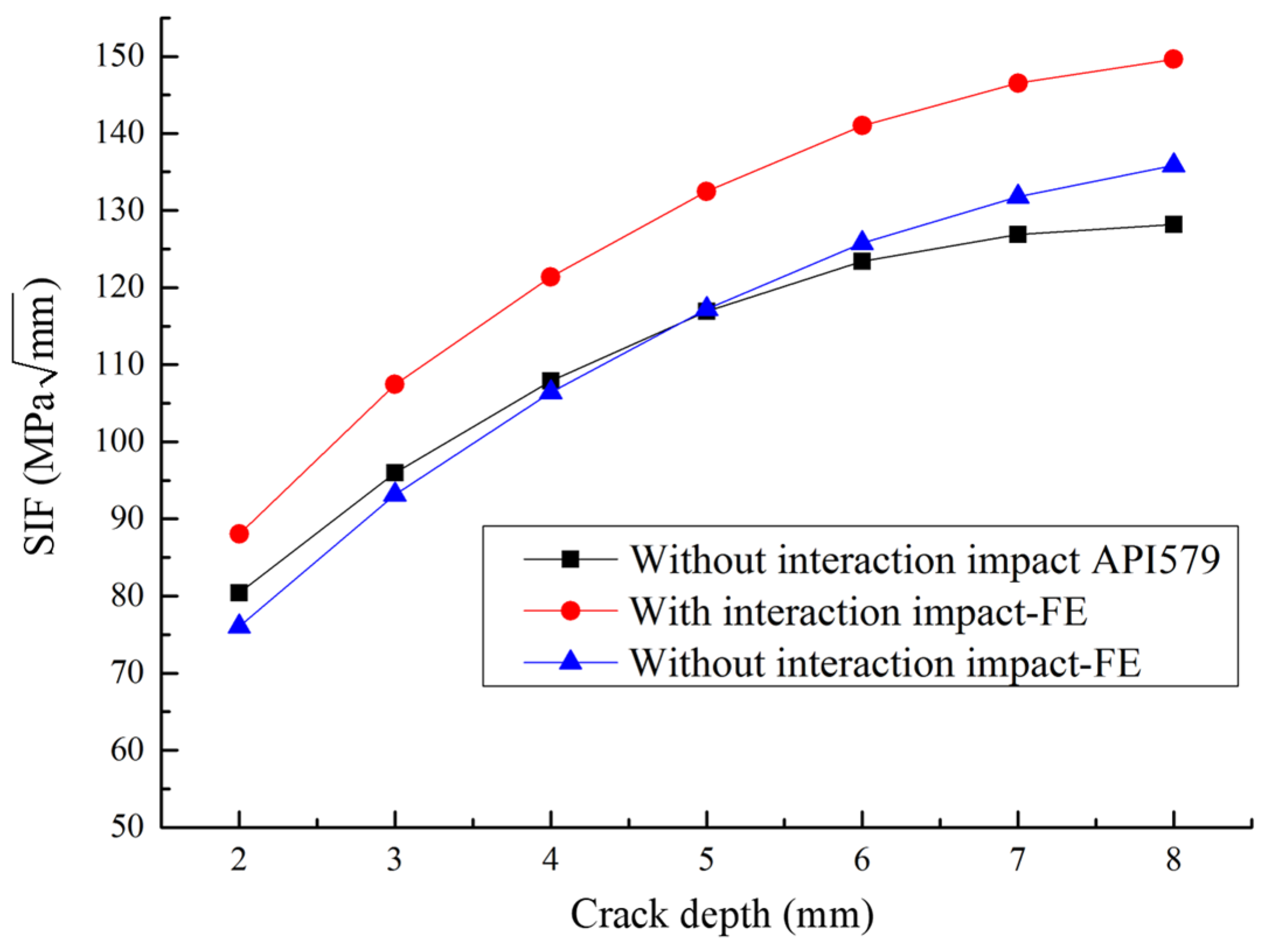
2.2. Validation of FEA
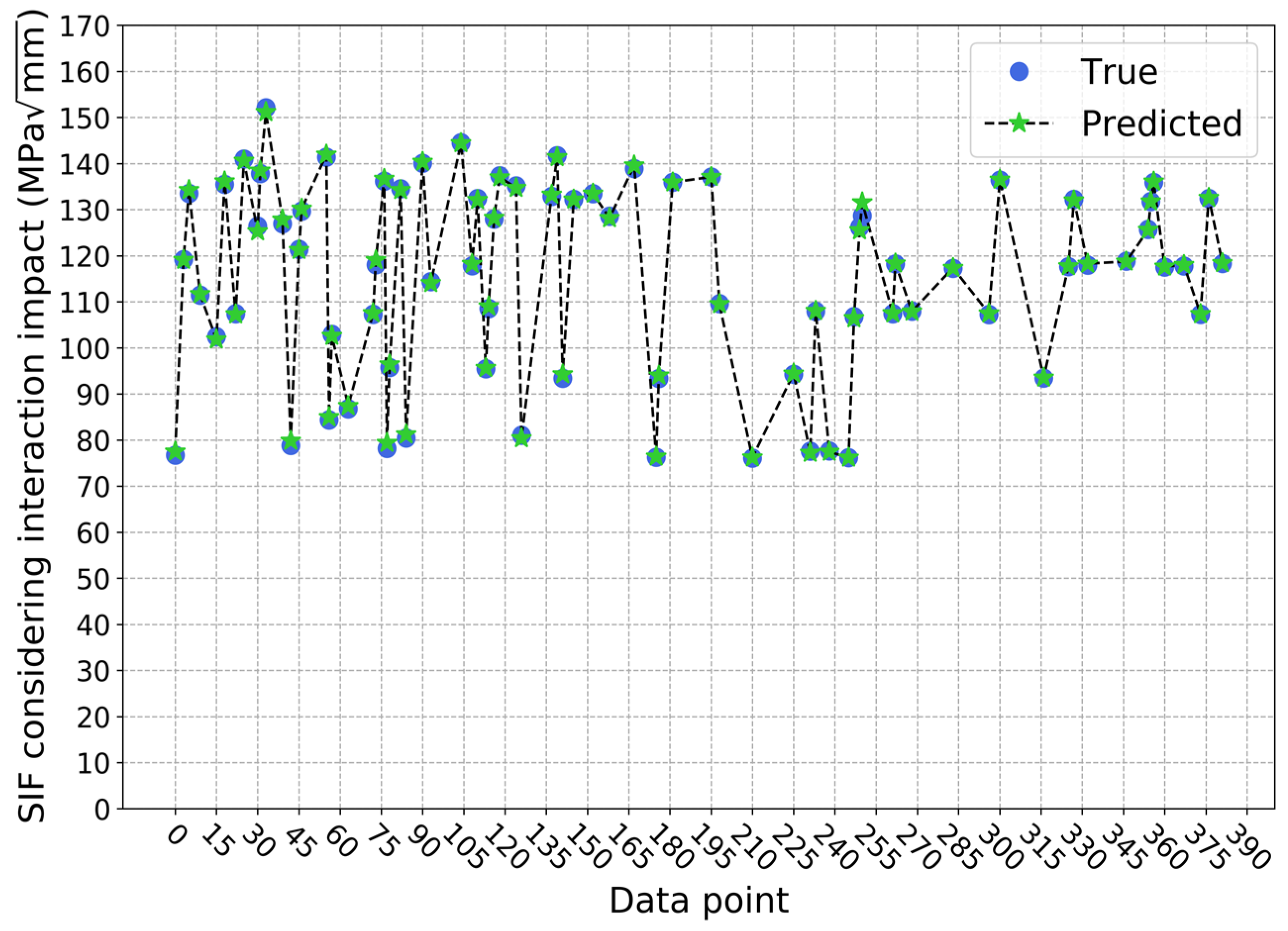
3. The Proposed Crack Propagation Method Based on Extreme Gradient-Boosting Algorithm
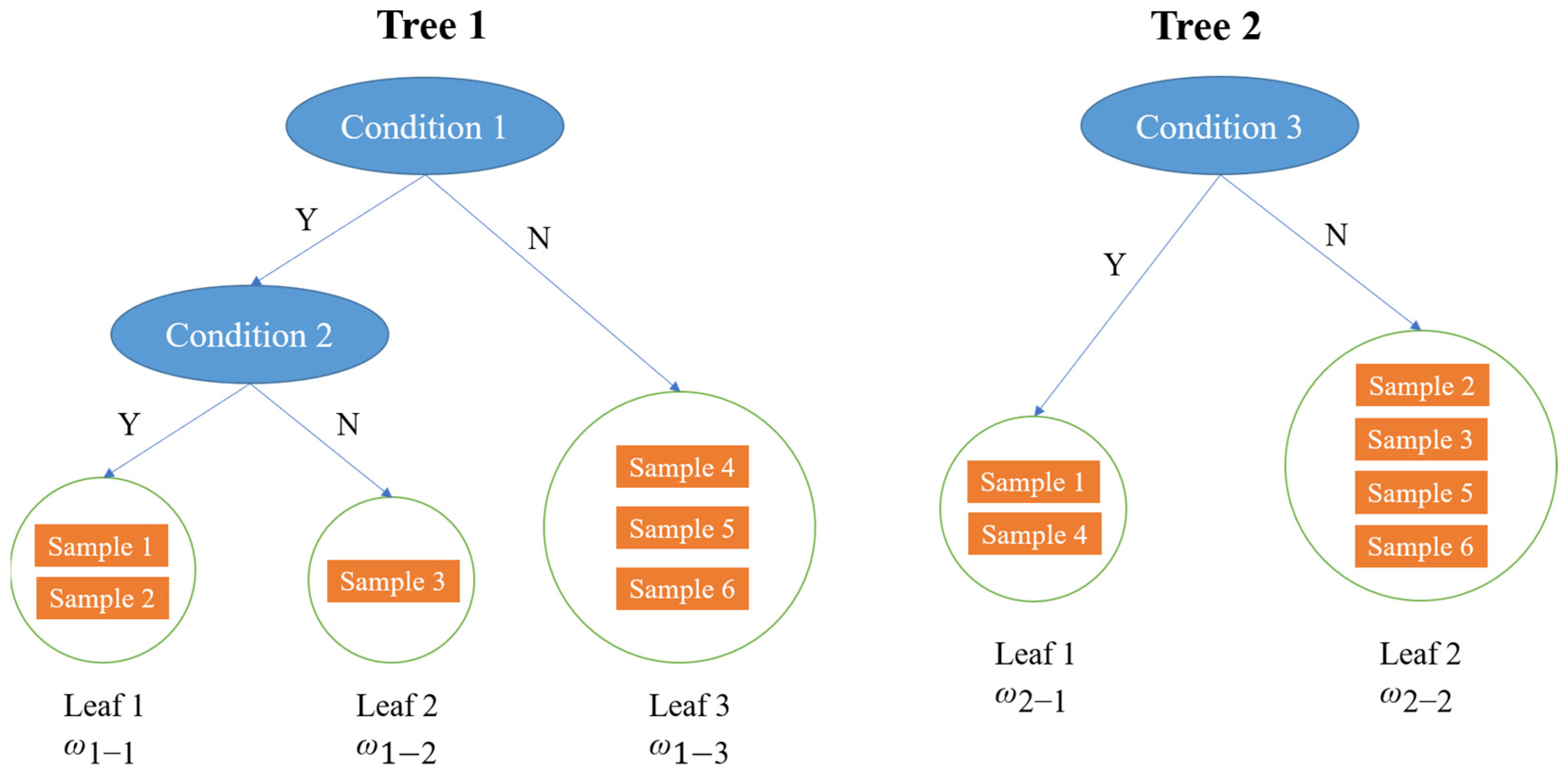
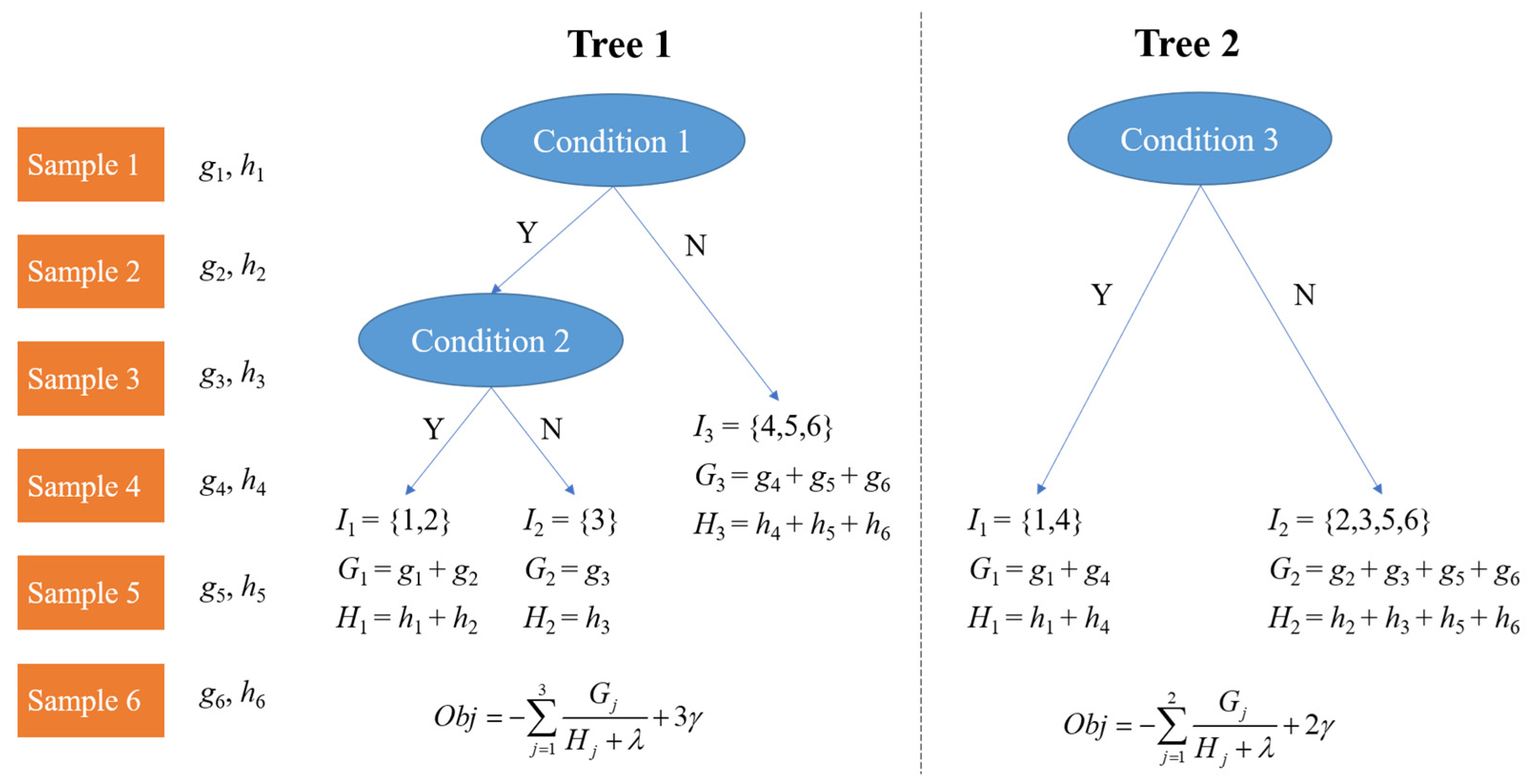
3.1. The Extreme Gradient-Boosting Model
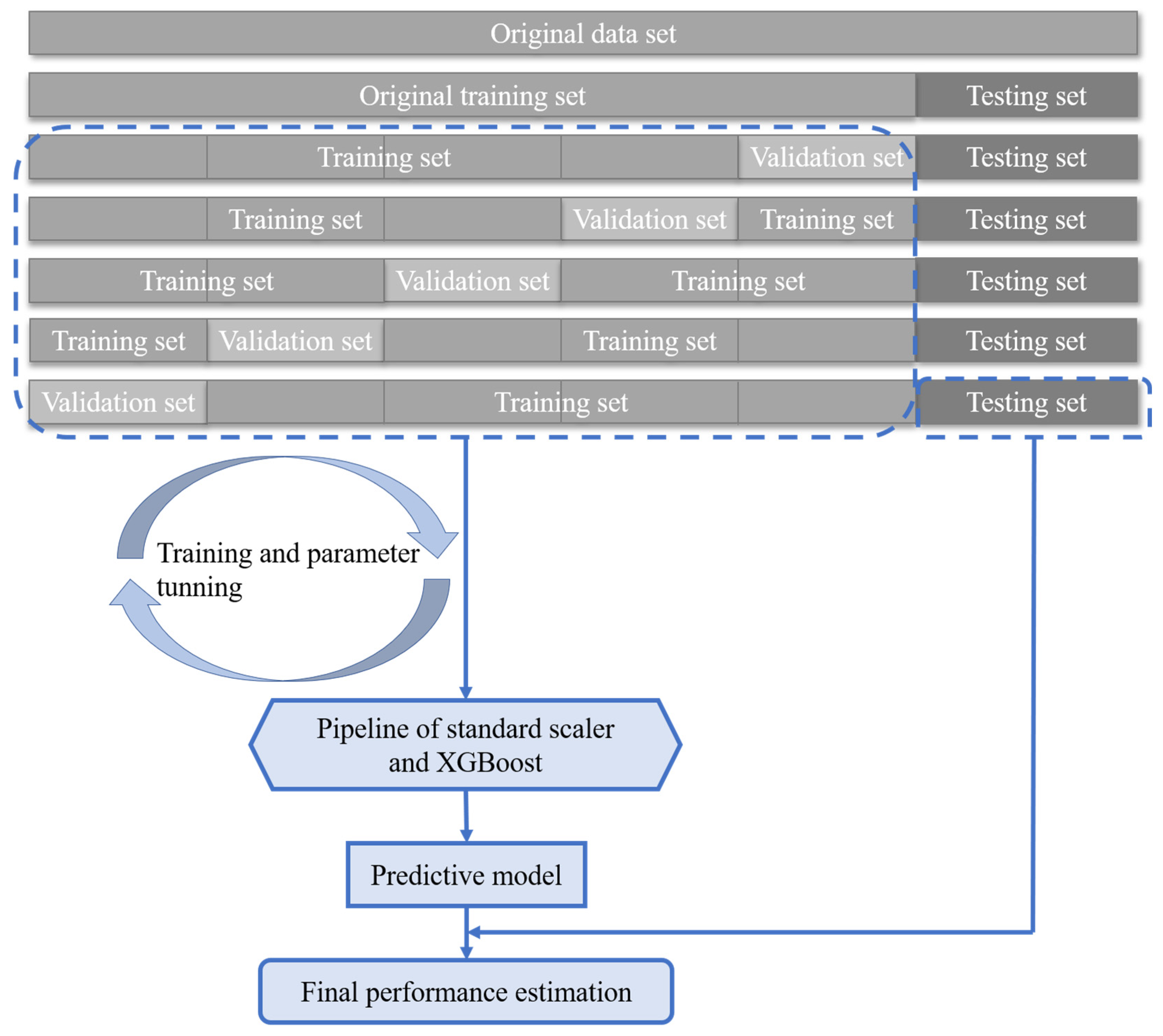
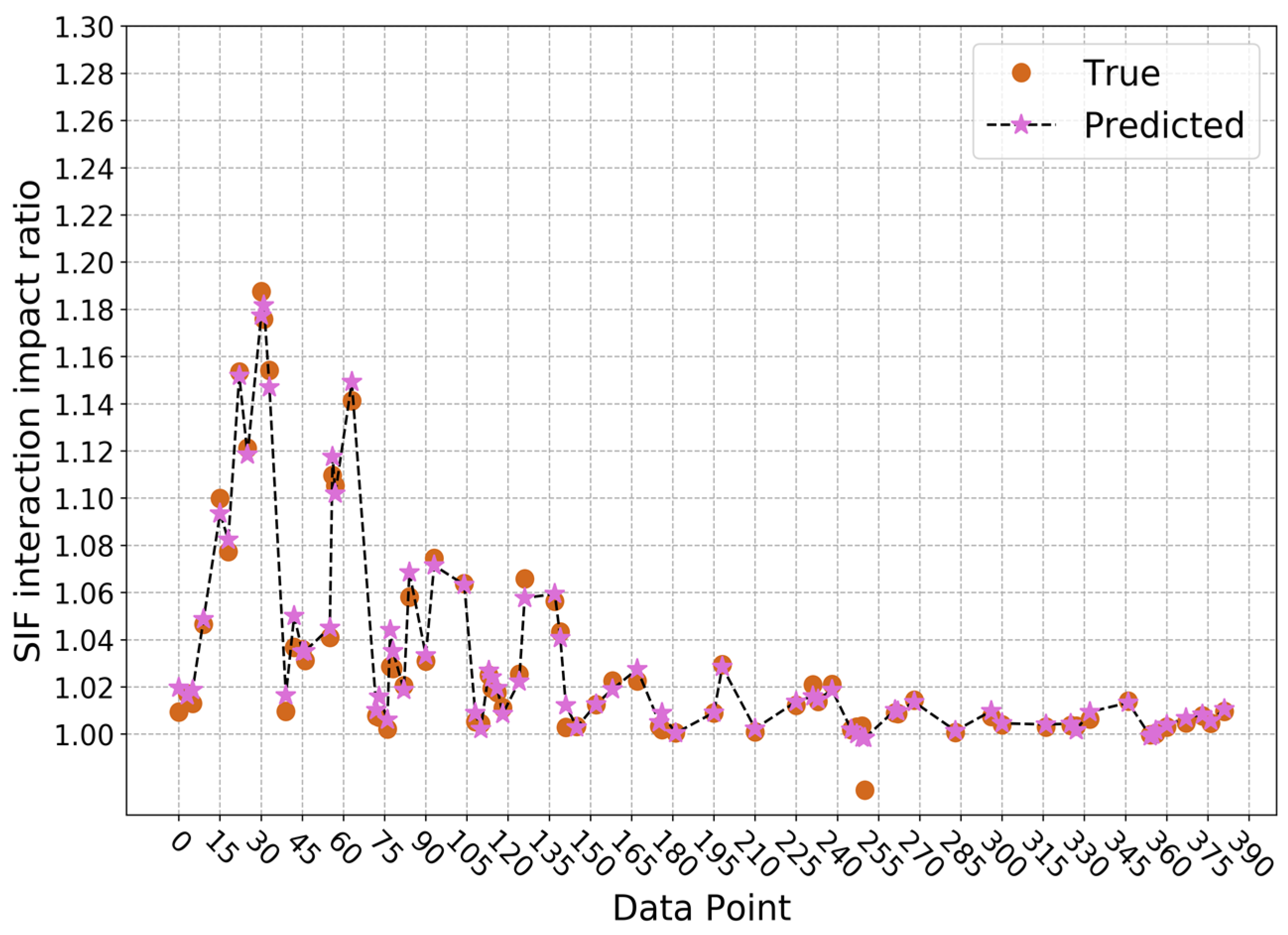
3.2. The Proposed Model Based on XGBoost
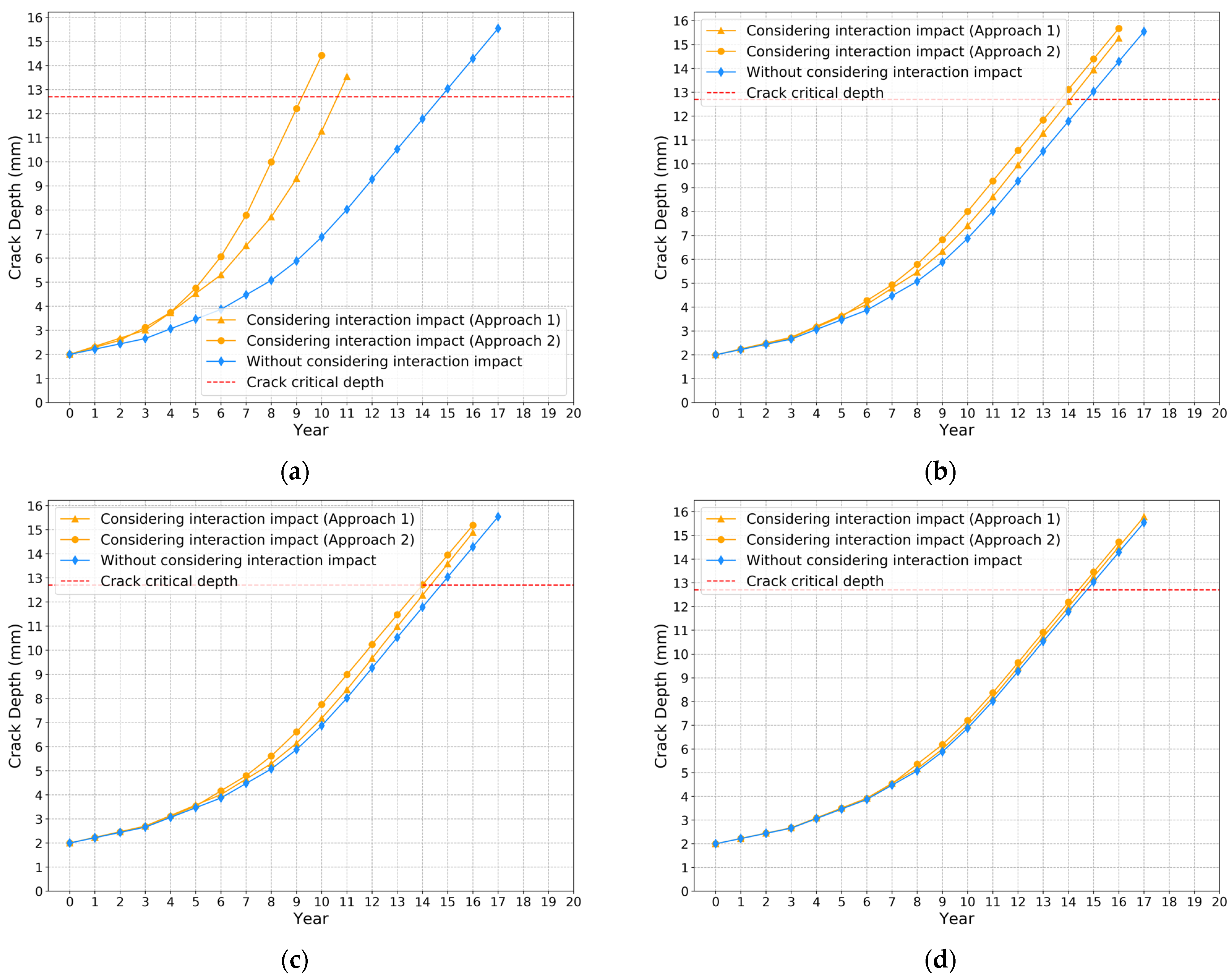
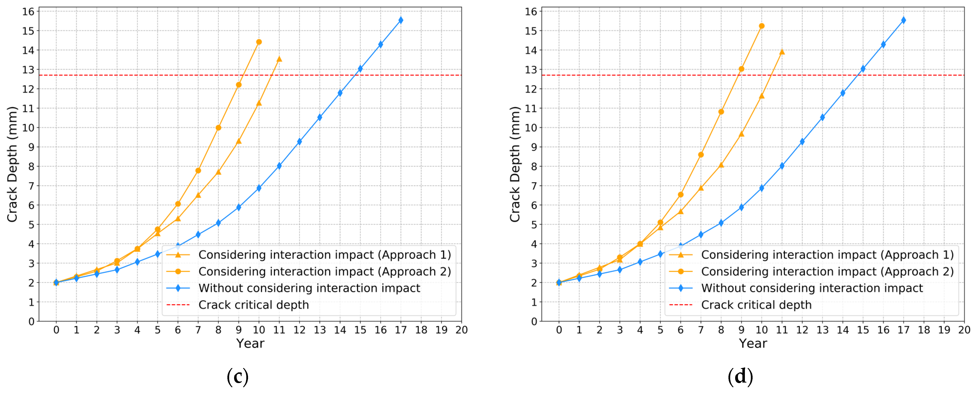
3.3. The Pipeline Corrosion and Fatigue Crack Growth Models
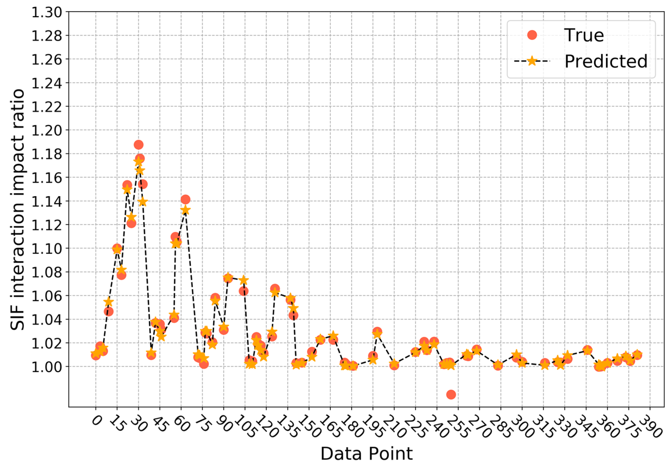
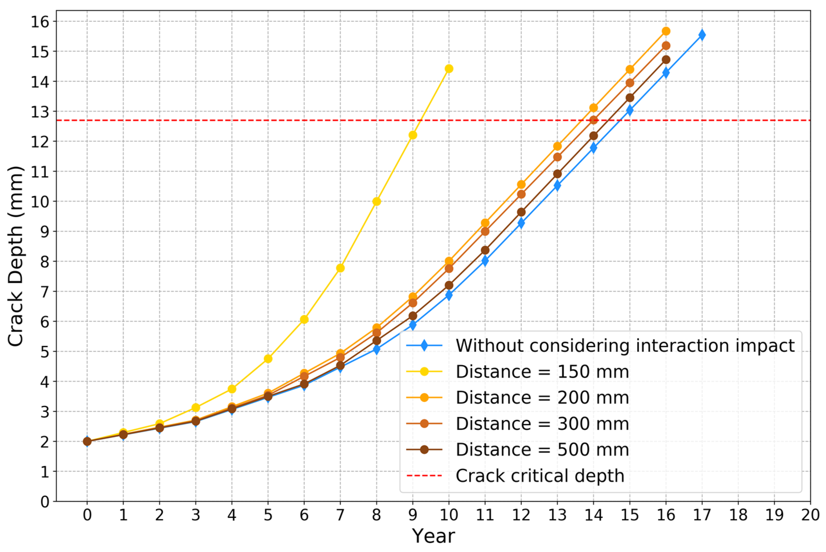
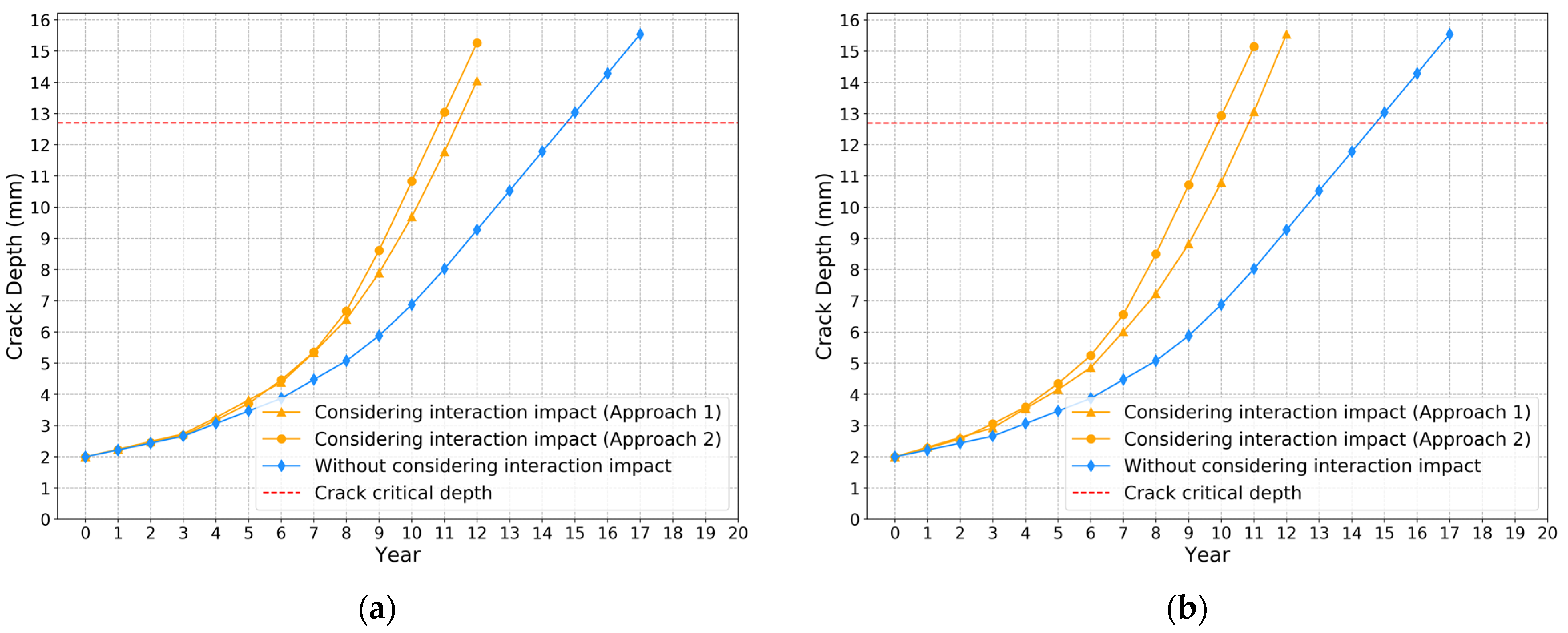
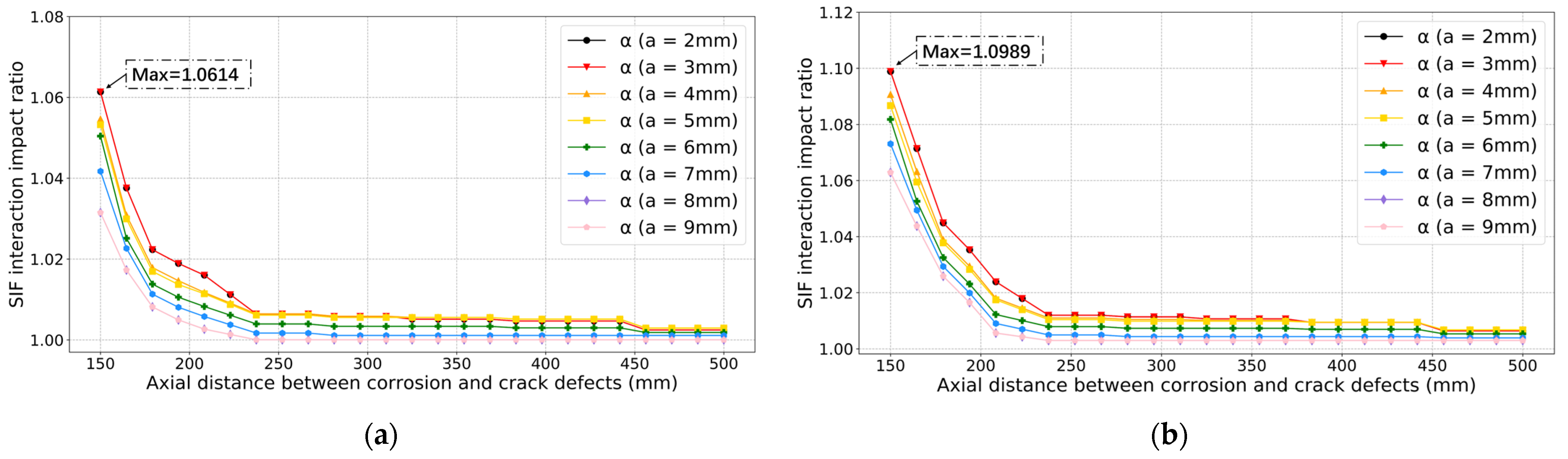
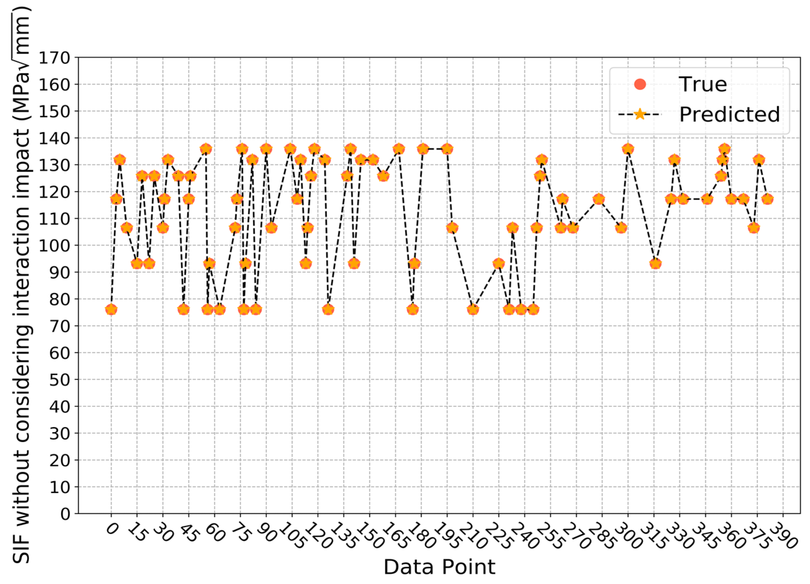
4. Results
5. Conclusions
Author Contributions
Funding
Data Availability Statement
Conflicts of Interest
Nomenclature
| p | pipeline internal pressure |
| a | crack depth |
| c | half crack length |
| Ri | pipeline internal radius |
| Ro | pipeline outer radius |
| Q | crack geometry parameter in API 579 |
| G0, G1, G2, G3, G4, M1, M2, M3, Ai,j ({0,1,2,3,4,5,6}, {0,1}), β | influence coefficients in API 579 |
| ϕ | included angle in API 579 |
| Obj | objective function of XGBoost |
| Θ | parameters obtained from the training processing in XGBoost |
| training error in XGBoost | |
| regularization term in XGBoost | |
| S | training dataset |
| l | training error of each sample in XGBoost |
| i-th sample | |
| target output of the i-th sample | |
| predicted output of the i-th sample | |
| z | number of features in the dataset |
| n | number of samples in the training dataset |
| V | number of classification and regression trees in XGBoost |
| v | v-th classification and regression tree in XGBoost |
| weights of samples falling on the leaf in the v-th tree | |
| F | function space of all the classification and regression trees in XGBoost |
| first-order derivative of training error for i-th sample in XGBoost | |
| second-order derivative of training error for i-th sample in XGBoost | |
| w | weight vector of leaves in classification and regression tree |
| T | number of leaves in classification and regression tree |
| q | mapping relationship between the leaves in classification and regression tree (viz. the structure of the tree) |
| γ | coefficient for number of leaves in regularization term in XGBoost |
| λ | coefficient for L2 norm of leaf weights in regularization term in XGBoost |
| instance set in leaf j | |
| Gj | sum of first-order derivatives of training error for leave j in XGBoost |
| Hj | sum of second-order derivatives of training error for leave j in XGBoost |
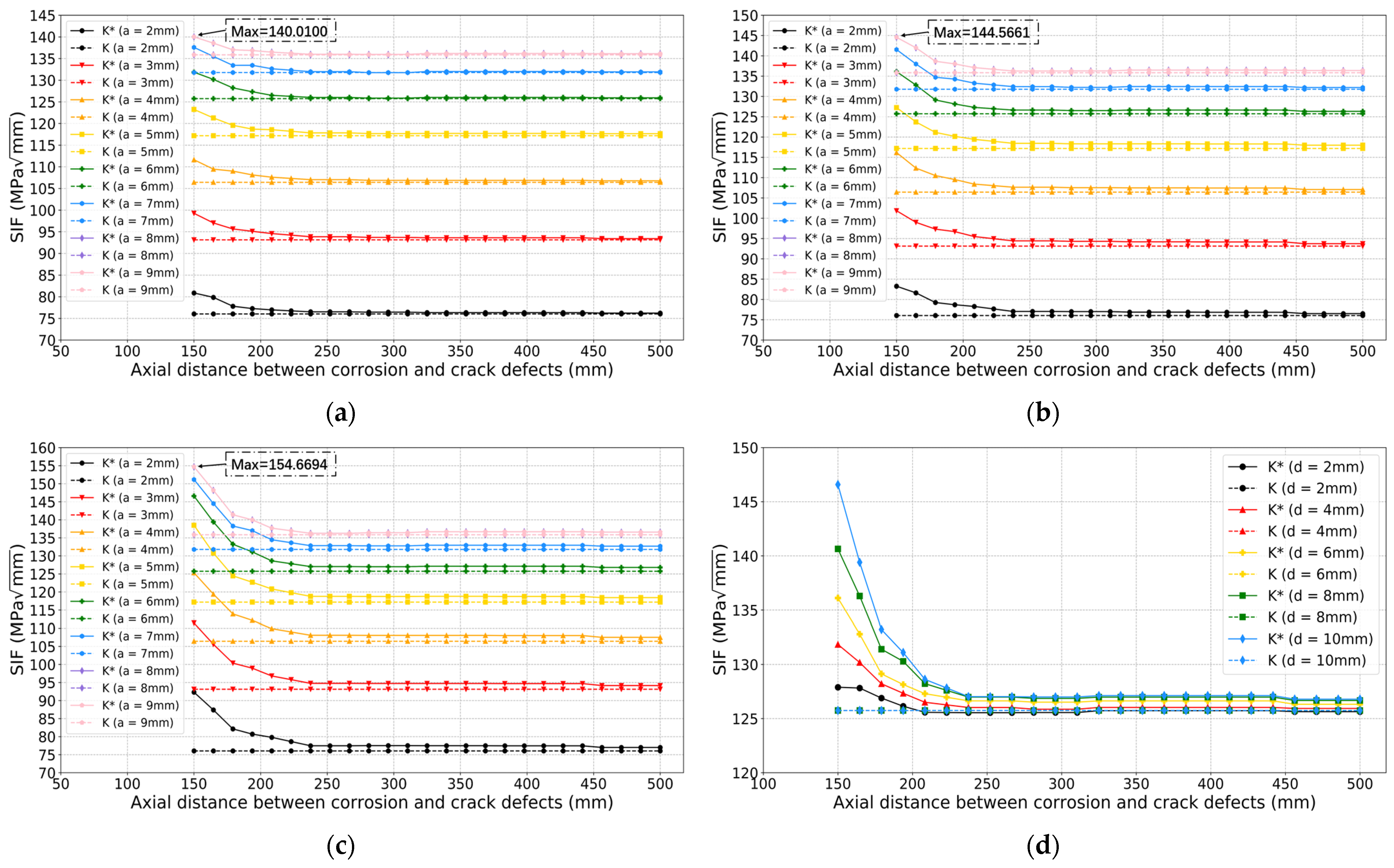
| K | SIF without considering interaction impact |
| K* | SIF considering interaction impact |
| α | interaction impact ratio |
| d | corrosion depth |
| d0 | corrosion initial depth |
| gd | growth rate of corrosion depth |
| t | propagation time |
| m, C | material parameters in Paris’ law |
| N | loading cycles |
| ΔK | the range of SIF |
References
- Vanaei, H.R.; Eslami, A.; Egbewande, A. A review on pipeline corrosion, in-line inspection (ILI), and corrosion growth rate models. Int. J. Press. Vessel. Pip. 2017, 149, 43–54. [Google Scholar] [CrossRef]
- Kishawy, H.A.; Gabbar, H.A. Review of pipeline integrity management practices. Int. J. Press. Vessel. Pip. 2010, 87, 373–380. [Google Scholar] [CrossRef]
- Xie, M.; Tian, Z. A review on pipeline integrity management utilizing in-line inspection data. Eng. Fail. Anal. 2018, 92, 222–239. [Google Scholar] [CrossRef]
- Wang, H.; Yajima, A.; Castaneda, H. A stochastic defect growth model for reliability assessment of corroded underground pipelines. Process. Saf. Environ. Prot. 2019, 123, 179–189. [Google Scholar] [CrossRef]
- Ossai, C.I.; Boswell, B.; Davies, I. Markov chain modelling for time evolution of internal pitting corrosion distribution of oil and gas pipelines. Eng. Fail. Anal. 2016, 60, 209–228. [Google Scholar] [CrossRef] [Green Version]
- Bazán, F.A.V.; Beck, A. Stochastic process corrosion growth models for pipeline reliability. Corros. Sci. 2013, 74, 50–58. [Google Scholar] [CrossRef]
- Qin, H.; Zhang, S.; Zhou, W. Inverse Gaussian process-based corrosion growth modeling and its application in the reliability analysis for energy pipelines. Front. Struct. Civ. Eng. 2013, 7, 276–287. [Google Scholar] [CrossRef]
- Pan, D.; Liu, J.-B.; Cao, J. Remaining useful life estimation using an inverse Gaussian degradation model. Neurocomputing 2016, 185, 64–72. [Google Scholar] [CrossRef] [Green Version]
- Peng, W.; Li, Y.-F.; Yang, Y.-J.; Huang, H.-Z.; Zuo, M. Inverse Gaussian process models for degradation analysis: A Bayesian perspective. Reliab. Eng. Syst. Saf. 2014, 130, 175–189. [Google Scholar] [CrossRef]
- Witek, M. Gas transmission pipeline failure probability estimation and defect repairs activities based on in-line inspection data. Eng. Fail. Anal. 2016, 70, 255–272. [Google Scholar] [CrossRef]
- Xie, M.; Tian, Z. Risk-based pipeline re-assessment optimization considering corrosion defects. Sustain. Cities Soc. 2018, 38, 746–757. [Google Scholar] [CrossRef]
- Gong, C.; Zhou, W. First-order reliability method-based system reliability analyses of corroding pipelines considering multiple defects and failure modes. Struct. Infrastruct. Eng. 2017, 13, 1451–1461. [Google Scholar] [CrossRef]
- Benjamin, A.C.; Freire, L.F.; Vieira, R.D.; Cunha, D.J. Interaction of corrosion defects in pipelines e Part 1: Fundamentals. Int. J. Press. Vessel. Pip. 2016, 144, 56–62. [Google Scholar] [CrossRef]
- Benjamin, A.C.; Freire, L.F.; Vieira, R.D.; Cunha, D.J. Interaction of corrosion defects in pipelines e Part 2: MTI JIP database of corroded pipe tests. Int. J. Press. Vessel. Pip. 2016, 145, 41–59. [Google Scholar] [CrossRef]
- Amandi, K.; Diemuodeke, E.; Briggs, T. Model for remaining strength estimation of a corroded pipeline with interacting defects for oil and gas operations. Cogent Eng. 2019, 6, 1663682. [Google Scholar] [CrossRef]
- Sun, J.; Cheng, Y.F. Modelling of mechano-electrochemical interaction of multiple longitudinally aligned corrosion defects on oil/gas pipelines. Eng. Struct. 2019, 190, 9–19. [Google Scholar] [CrossRef]
- Soares, E.; Bruère, V.M.; Afonso, S.M.; Willmersdorf, R.B.; Lyra, P.R.; Bouchonneau, N. Structural integrity analysis of pipelines with interacting corrosion defects by multiphysics modeling. Eng. Fail. Anal. 2019, 97, 91–102. [Google Scholar] [CrossRef]
- Chen, Y.; Zhang, H.; Zhang, J.; Liu, X.; Li, X.; Zhou, J. Failure assessment of X80 pipeline with interacting corrosion defects. Eng. Fail. Anal. 2015, 47, 67–76. [Google Scholar] [CrossRef]
- Kuppusamy, C.S.; Karuppanan, S.; Patil, S.S. Buckling Strength of Corroded Pipelines with Interacting Corrosion Defects: Numerical Analysis. Int. J. Struct. Stab. Dyn. 2016, 16, 1550063. [Google Scholar] [CrossRef]
- Amaro, R.L.; Drexler, E.S.; Slifka, A.J. Fatigue crack growth modeling of pipeline steels in high pressure gaseous hydrogen. Int. J. Fatigue 2014, 62, 249–257. [Google Scholar] [CrossRef]
- Xie, M.; Bott, S.; Sutton, A.; Nemeth, A.; Tian, Z. An Integrated Prognostics Approach for Pipeline Fatigue Crack Growth Prediction Utilizing Inline Inspection Data. J. Press. Vessel. Technol. 2018, 140, 031702. [Google Scholar] [CrossRef] [Green Version]
- Okodi, A.; Lin, M.; Yoosef-Ghodsi, N.; Kainat, M.; Hassanien, S.; Adeeb, S. Crack propagation and burst pressure of longitudinally cracked pipelines using extended finite element method. Int. J. Press. Vessel. Pip. 2020, 184, 104115. [Google Scholar] [CrossRef]
- Zhang, Y.; Xiao, Z.; Luo, J. Fatigue crack growth investigation on offshore pipelines with three-dimensional interacting cracks. Geosci. Front. 2018, 9, 1689–1697. [Google Scholar] [CrossRef]
- Hu, J.; Tian, Y.; Teng, H.; Yu, L.; Zheng, M. The probabilistic life time prediction model of oil pipeline due to local corrosion crack. Theor. Appl. Fract. Mech. 2014, 70, 10–18. [Google Scholar] [CrossRef]
- Lu, B.; Song, F.; Gao, M.; Elboujdaini, M. Crack growth prediction for underground high pressure gas lines exposed to concentrated carbonate–bicarbonate solution with high pH. Eng. Fract. Mech. 2011, 78, 1452–1465. [Google Scholar] [CrossRef]
- Sekhar, A.S. Multiple cracks effects and identification. Mech. Syst. Signal Process. 2008, 22, 845–878. [Google Scholar] [CrossRef]
- Chen, T.; Guestrin, C. XGBoost: A Scalable Tree Boosting System; ACM: New York, NY, USA, 2016; Volume 16, pp. 13–17. [Google Scholar]
- Nielsen, A.; Mallet-Paret, J.; Griffin, K. Probabilistic Modeling of Crack Threats and the Effects of Mitigation. In Proceedings of the 2014 10th International Pipeline Conference, Calgary, AB, Canada, 29 September–3 October 2014; Volume 3, p. V003T12A021. [Google Scholar]
- Sutton, A.; Hubert, Y.; Textor, S.; Haider, S. Allowable Pressure Cycling Limits for Liquid Pipelines. In Proceedings of the 2014 10th International Pipeline Conference, Calgary, AB, Canada, 29 September–3 October 2014; Volume 2, p. V002T06A058. [Google Scholar]
- Waheed, B.; McAuliff, K.; Bhuyan, G. Knowledge Gained From a Five-Year Regulatory Compliance Assurance Process for Operators’ Pipeline Integrity Management Programs. In Proceedings of the 2016 10th International Pipeline Conference, Calgary, AB, Canada, 26–30 September 2016; Volume 50266, p. V002T01A006. [Google Scholar]


| Input Variables | Output Variables |
|---|---|
| Crack length | SIF considering interaction impact (K*) |
| Crack depth | SIF without considering interaction impact (K) |
| Corrosion length | Interaction impact ratio (α) |
| Corrosion depth | |
| Axial distance between crack and corrosion defects |
| Parameters | Adjusting Ranges |
|---|---|
| Number of gradient-boosted trees | {40,50,60,70,80,90,100,110} |
| Maximum depth of a tree | {3,4,5,6,7,8,9,10} |
| Minimum sum of instance weight needed in a child | {1,2,3,4,5,6} |
| L1 regularization term on weights | {0.05,0.1,1,2,3} |
| L2 regularization term on weights | {0.05,0.1,1,2,3} |
Publisher’s Note: MDPI stays neutral with regard to jurisdictional claims in published maps and institutional affiliations. |
© 2022 by the authors. Licensee MDPI, Basel, Switzerland. This article is an open access article distributed under the terms and conditions of the Creative Commons Attribution (CC BY) license (https://creativecommons.org/licenses/by/4.0/).
Share and Cite
Xie, M.; Wang, Y.; Xiong, W.; Zhao, J.; Pei, X. A Crack Propagation Method for Pipelines with Interacting Corrosion and Crack Defects. Sensors 2022, 22, 986. https://doi.org/10.3390/s22030986
Xie M, Wang Y, Xiong W, Zhao J, Pei X. A Crack Propagation Method for Pipelines with Interacting Corrosion and Crack Defects. Sensors. 2022; 22(3):986. https://doi.org/10.3390/s22030986
Chicago/Turabian StyleXie, Mingjiang, Yifei Wang, Weinan Xiong, Jianli Zhao, and Xianjun Pei. 2022. "A Crack Propagation Method for Pipelines with Interacting Corrosion and Crack Defects" Sensors 22, no. 3: 986. https://doi.org/10.3390/s22030986
APA StyleXie, M., Wang, Y., Xiong, W., Zhao, J., & Pei, X. (2022). A Crack Propagation Method for Pipelines with Interacting Corrosion and Crack Defects. Sensors, 22(3), 986. https://doi.org/10.3390/s22030986