Article

Rayleigh-Wave Dispersion Analysis and Inversion Based on the Rotation

“MWMC” Group, School of Geophysics and Information Technology, China University of Geosciences, Beijing 100083, China
*
Author to whom correspondence should be addressed.
Sensors 2022, 22(3), 983; https://doi.org/10.3390/s22030983
Submission received: 6 December 2021 / Revised: 20 January 2022 / Accepted: 22 January 2022 / Published: 27 January 2022
(This article belongs to the Special Issue Data Acquisition and Analysis of Seismic Noise)

Abstract

:
Rotational observation is essential for a comprehensive description of the ground motion, and can provide additional wave-field information. With respect to the three typical layered models in shallow engineering geology, under the assumption of linear small deformation, we simulate the 2-dimensional radial, vertical, and rotational components of the wave fields and analyze the different characteristics of Rayleigh wave dispersion recorded for the rotational and translational components. Then, we compare the results of single-component inversion with the results of multi-component joint inversion. It is found that the rotational component has wider spectral bands and more higher modes than the translational components, especially at high frequencies; the rotational component has better anti-interference performance in the noisy data test, and it can improve the inversion accuracy of the shallow shear-wave velocity. The field examples also show the significant advantages of the joint utility of the translational and rotational components, especially when a low-velocity layer exists. Rotational observation shall be beneficial for shallow surface-wave exploration.

1. Introduction

Surface-wave exploration is an important method in the field of geophysics used for the detection of the shallow shear-wave velocity structure of the earth, and includes single-station method, two-station method [1], two-plane-wave method [2], ambient noise tomography based on passive source [3], microtremor method [4,5,6], rotational seismic method [7,8], and the most widely used method in the seismic exploration—multi-channel analysis of surface waves (Rayleigh and Love waves) [9,10].
In recent years, numerous experimental studies have used high-speed railway vibration signals for extracting the dispersion curves of the surface waves [11] and used the surface waves detected by an urban telecommunication optic-fiber cable to obtain the shallow velocity structure [12]. Due to the poor applicability of the fundamental-mode surface waves for complex media (containing a low-velocity interlayer and a high-velocity interlayer) [13], the joint utilization of the fundamental and the higher modes has attracted extensive attention [14,15,16,17] and led to better applications [18,19,20,21]. However, the effective identification and accurate extraction of different modes and overcoming the difficulty of misidentification of Rayleigh-wave modes caused by the phenomenon of “mode kissing” has become the main problem faced by the traditional SPAC (spatial autocorrelation) method [22,23,24]. The high-resolution linear Radon transform [25] and the complex vector method, which jointly use the multi-component seismic data, show good results in extracting the surface-wave dispersion curves of different modes [26]. The joint use of the radial and vertical components of seismic translational motions to invert the shallow velocity structure has also been widely used [27,28,29,30,31].
With the development of the rotational seismology, the joint use of translational and rotational components to detect the shallow shear-wave velocity structure has become one of the hotspots in the field of engineering and shallow seismic exploration [32,33]. Six-component (translational- and rotational-component) geophones and seismometers are gradually utilized in these fields [34,35]. However, rotational seismometers’ low sensitivity, large background noise, narrow frequency bandwidths, and high cost still limited their popularization and application [36,37,38]. They are expensive for oil and engineering exploration. There are some methods to obtain the rotational motions indirectly, such as the two-point difference method, which requires the dense seismic array or network [39]. Moreover, wireless seismic geophones make the dense seismic network efficient owing to small logistic and sufficient flexibility [40,41,42]. Therefore, in the near field of strong earthquakes, the rotational motions can be obtained by the wireless seismic geophone resultant.
The comprehensive observation of seismic motions has plenty of advantages on surface wave inversion. The surface-wave phase velocity can be obtained using the rotational rate measured by the rotational seismometers and the acceleration measured by the translational geophone on a single location without an array of geophones [7]. The apparent shear-wave speed, which is defined by the rms (root-mean-square) amplitude ratio of the translational component and rotational component, can be used for single-station local S-wave velocity tomography [32]. Additionally, the energy of surface waves is stronger than that of body waves on the rotational components, which can be used for surface wave inversion [43].
However, compared with the translational seismic method, other advantages of the rotational observation are attempted to be clarified in this paper. Aimed at three typical layered models in shallow engineering geology, we analyze the Rayleigh-wave dispersion characteristics of the rotational component differing from the translational components through theoretical simulations. In addition, we compare the single-component inversion with the multi-component joint inversion with the numerical and field data, which are calculated with the two-point difference method by using the translational field seismic data. It is demonstrated that the understanding and utilization of the surface-wave dispersion curves on rotational components is helpful to improve the detection accuracy of the shallow shear-wave velocity structure.

2. Theoretical Foundations

2.1. Calculation of the Rotational Component

The motion of a particle includes translation, rotation, and deformation. In space, the motion of an arbitrary point can be expressed as three translational components along the axis and three rotational components around the axis (Figure 1) [44]. In the traditional linear elastodynamics theory, the rotational tensor is defined as follows:
r = 1 2 × u
where r is the rotational tensor, u is the displacement. It is obviously that the rotation tensor is half of the curl of the displacement vector.
In order to completely describe the ground motion, six degrees of freedom in a three dimensional world are required, as shown in Table 1 [43]. In the two-dimensional case, it becomes three components—the radial (ux), vertical (uz), and yaw (ry) components. We analyze the wave-field characteristics of three components under the assumption of two-dimensional linear small deformation and use the surface-wave dispersion curves extracted from different components to predict shear-wave phase velocity.
Since the actual rotational observation is mainly the rotational rate, it is necessary to obtain the rotation rate in the numerical simulation by the derivative of Formula (1) with respect to time (t). Further, the rotation rate Ry can be obtained through discrete difference calculation by the wave-field velocity, which can be expressed as:
R y ( x , z , t ) = 1 2 ( v x ( x , z + Δ z , t ) v x ( x , z , t ) Δ z v z ( x + Δ x , z , t ) v z ( x , z , t ) Δ x )
where R y ( x , z , t ) is the calculated rotational value, which is used in our simulation analyses, Δ x and Δ z are 0.2 m, v x ( x , z , t ) and v x ( x , z + Δ z , t ) are the radial component velocities at different depths, and v z ( x , z , t ) and v z ( x + Δ x , z , t ) are the vertical component velocities at different points.

2.2. Rayleigh Wave Simulation

In this paper, the two translational components of surface wave are synthesized by the convolution of the dispersion curves and eigenfunction (modal summation method) [45] with the CPS (The Computer Programs in Seismology) software [46], because the method is based on the analytical solution of the surface wave and the surface-wave fields are considered as pure. Then, the rotational component wave fields are calculated with translational records according to the Formula (2), although the rotational components can be simulated with the finite difference method [47,48]. While in the real data testing, we use the two-point difference method [49] to obtain the rotational component Ry, since the rotational seismometers are not popular and there is usually a lack of rotational observation in the field of engineering seismic prospecting.

2.3. Method of Surface-Wave Dispersive Energy Imaging and Surface-Wave Inversion

High-resolution Radon transform is used to calculate surface-wave dispersive energy in this paper. The Radon coefficients are obtained with formula [25]:
( λ I + W m H L H W d H W d L W m 1 ) m ˜ = W m H L H W d H W d d
where m ˜ = W m m , W d , and W m are the weighted matrices, L and L H are the operator matrices, λ is the regularization parameter, and I is the identity matrix. m is the Radon coefficient in the frequency–velocity (f–v) domain, which is a complex number. d is the seismic data in the frequency–offset domain.
The dispersive energy in the f–v domain can be imaged with the module of the Radon coefficients [14]. Then, the imaged energy is normalized at each frequency, which can remove the effect of the source wavelet spectrum [26].
Furthermore, we extract the surface-wave dispersion curves from different components and inverse the shallow underground velocity structure using the Rayleigh wave inversion program of CPS software—the surf96 module. Under the smoothness constraint, a damped least-square inversion method is used to find the most suitable model matching the observed values and invert the velocity structure by the dispersion curves of surface waves.

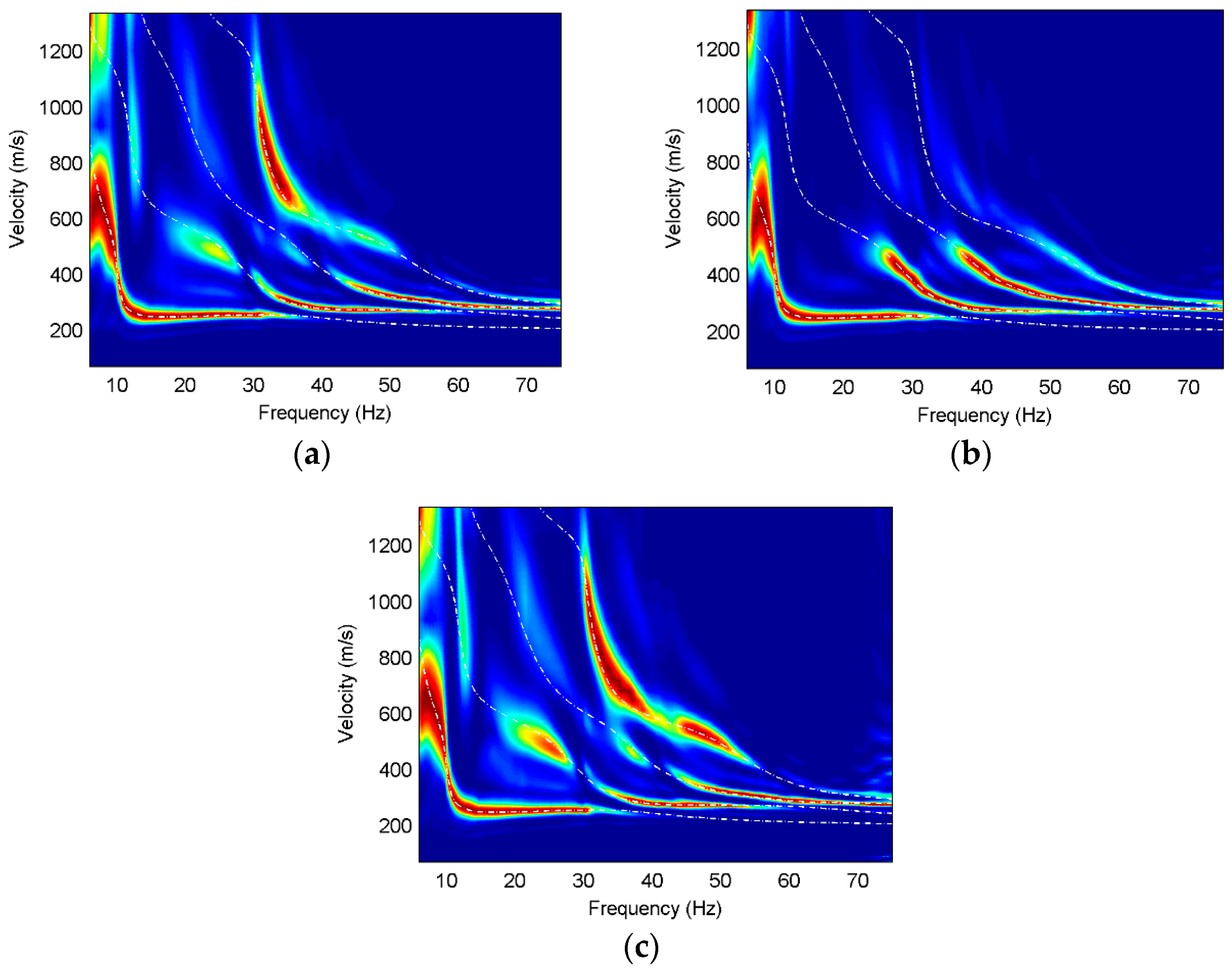
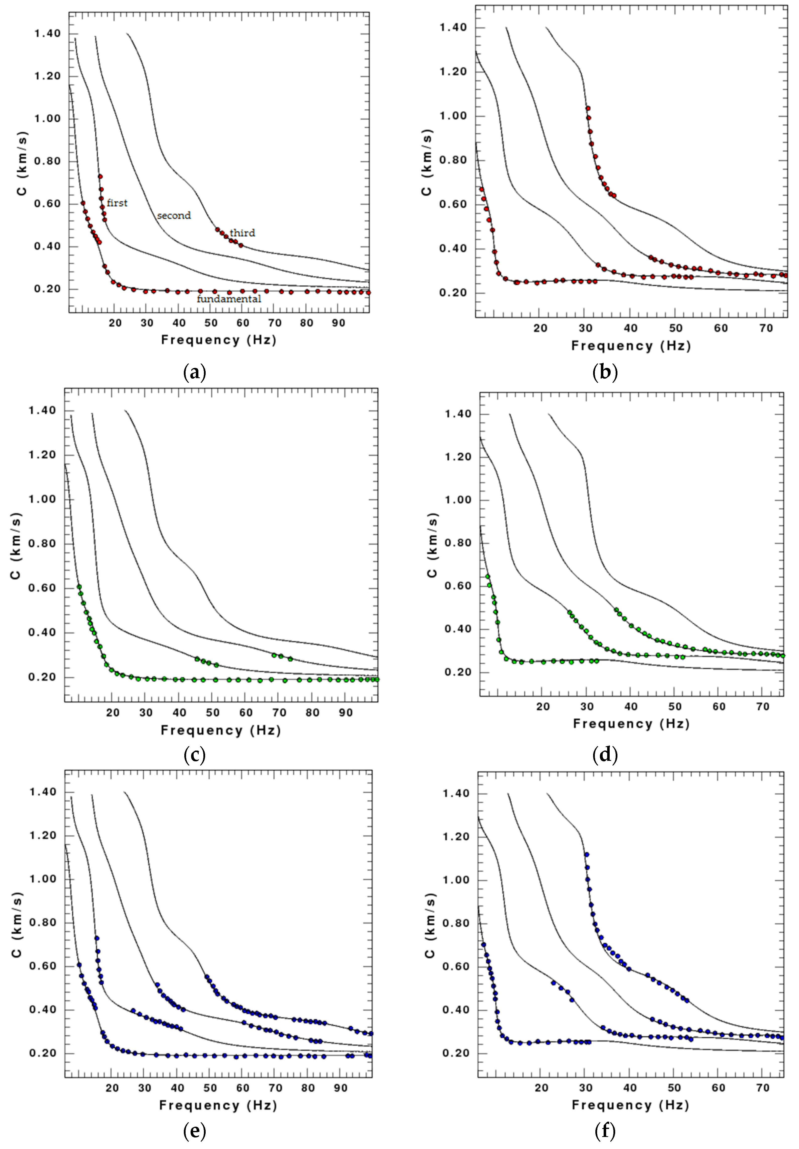
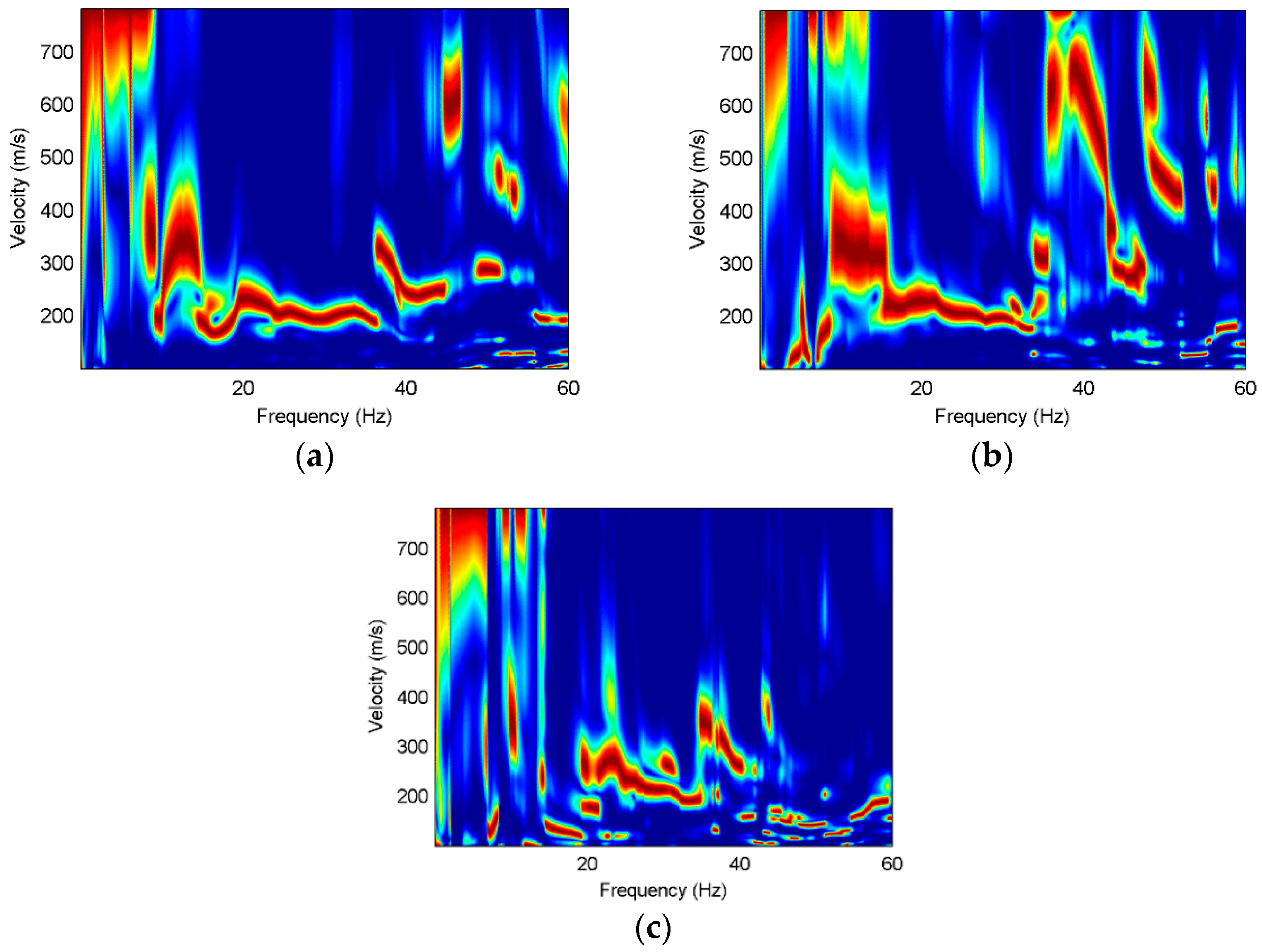
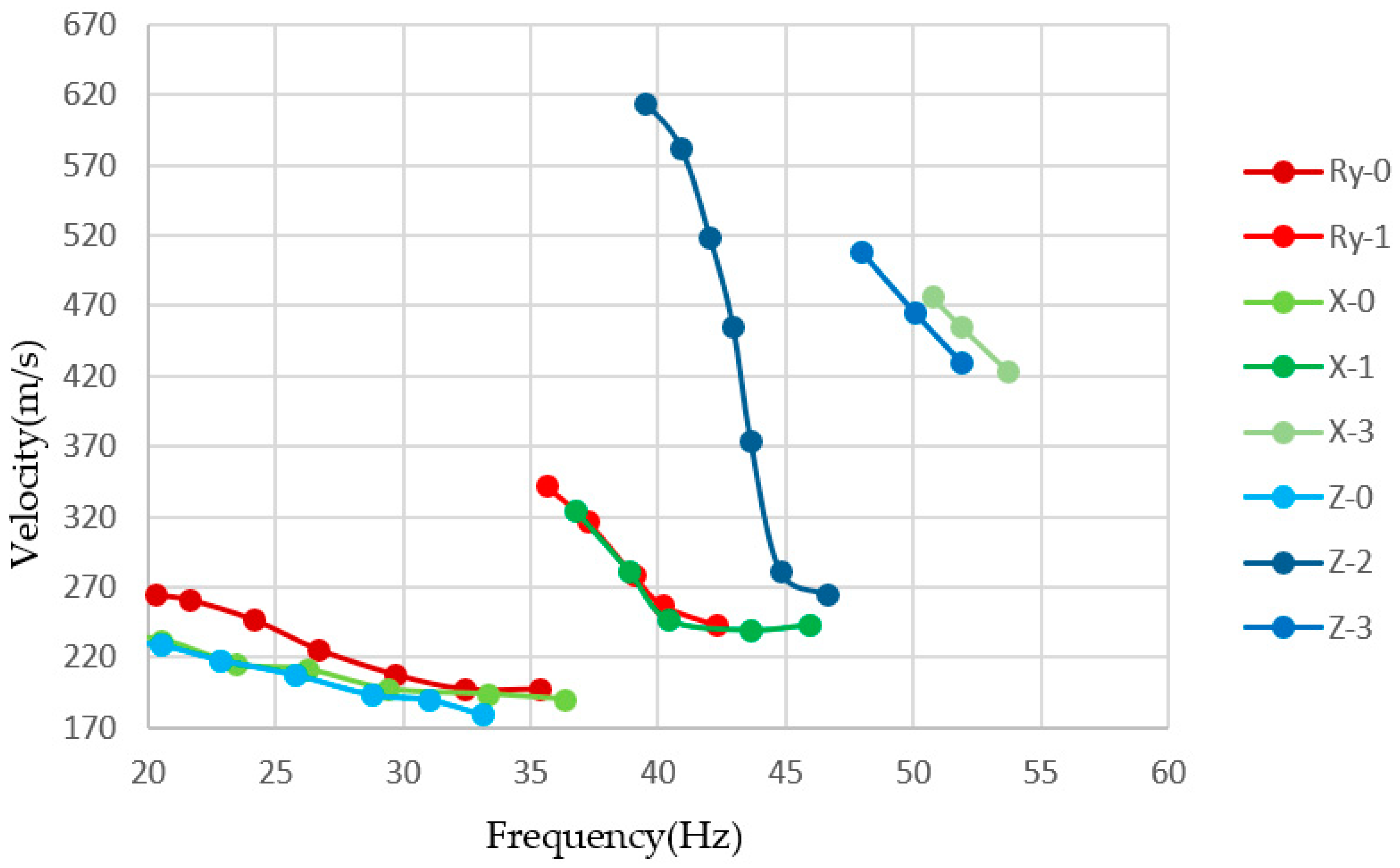
3. The Wave-Field Characteristics of the Typical Shallow Models

Considering the generality of the discussion, we define three typical models based on the common geological structures in shallow engineering geology—horizontal layered model with velocity increasing with depth and layered model containing low-velocity interlayer or containing high-velocity interlayer. The model parameters are shown in Table 2. We simulate the surface-wave fields with a vertical concentrated force source (a 25 Hz Ricker wavelet) at the surface. With the sample interval of 0.5 ms, there are 49 receivers arrayed in line at the surface with 1 m intervals and the nearest offset is 5 m.
The synthetic data for Model 2 are illustrated in this paper in Figure 2. It can be clearly seen that there is strong Rayleigh wave energy in the shape of a broom on the three components. The energy of Rayleigh waves is much stronger on the vertical and rotational components than that on the radial component.
In order to further analyze the Rayleigh wave characteristics on different components, we use high-resolution linear Radon transform [25] to obtain the multi-mode surface-wave dispersive spectra. The dispersions of three components are normalized at each frequency and the theoretical dispersion curves of different modes are calculated for contrast, as shown in Figure 3, Figure 4 and Figure 5.
It can be found that obvious fundamental and higher modes exist on the three components, and the dispersion curves for different models basically correspond well with their theoretical dispersion curves. The fundamental mode of Model 1 is dominant on all components, and the fundamental mode on the vertical component has energy distribution at 15–18 Hz, while that on the other two components is discontinuous at the same frequencies. The first higher mode on the radial and rotational components has comparative amplitude responses at 10–15 Hz frequencies, while not all higher modes are present in the dispersion images. The higher modes on the translational components have much weaker energy than those on the rotational component at 15–100 Hz frequencies and the higher-mode dispersion curves can hardly be extracted from the translational components. In contrast, the higher modes, especially the third higher mode, have strong energy on the rotational component and the dispersion information is relatively complete.
The fundamental modes of Model 2 on three components are similar while the higher modes have different characteristics on different components. The first higher mode and the second higher mode on the vertical component have much stronger energy than those on the other two components at the frequencies of 25–40 Hz, while the third higher mode is almost absent on the vertical component, but dominant on the radial and translational components. The dispersion images on the rotational component are slightly better than those on the radial component of Model 2, which is reflected in the energy of the first higher mode at 20–30 Hz frequencies, the energy of the second higher mode at 32–40 Hz frequencies, and the energy of the third higher mode at 40–52 Hz frequencies. It is obvious that the rotation has wider spectral bands than the translations in the horizontal layered model containing a low-velocity interlayer.
In Model 3, the higher modes on the vertical component have weaker energy than the other components. It can be observed that the dispersive energy of the vertical component at 10–15 Hz frequencies is misidentified as the fundamental mode, which is the phenomenon of mode misidentification. However, mode misidentification can be overcome using multi-component seismic data. The fundamental-mode and higher-mode dispersion curves on the radial and rotational components match well with the theoretical dispersion curves. The energy of the higher modes on the rotational component is much stronger than that on the radial component. Furthermore, the dispersive energy of the higher modes on the rotational component has wider frequency bands and more high-frequency information than that on the radial component.
Therefore, we can deduce that the rotational components are helpful to pick up dispersion curves of different modes, which is beneficial for the surface-wave inversion and geological interpretation.

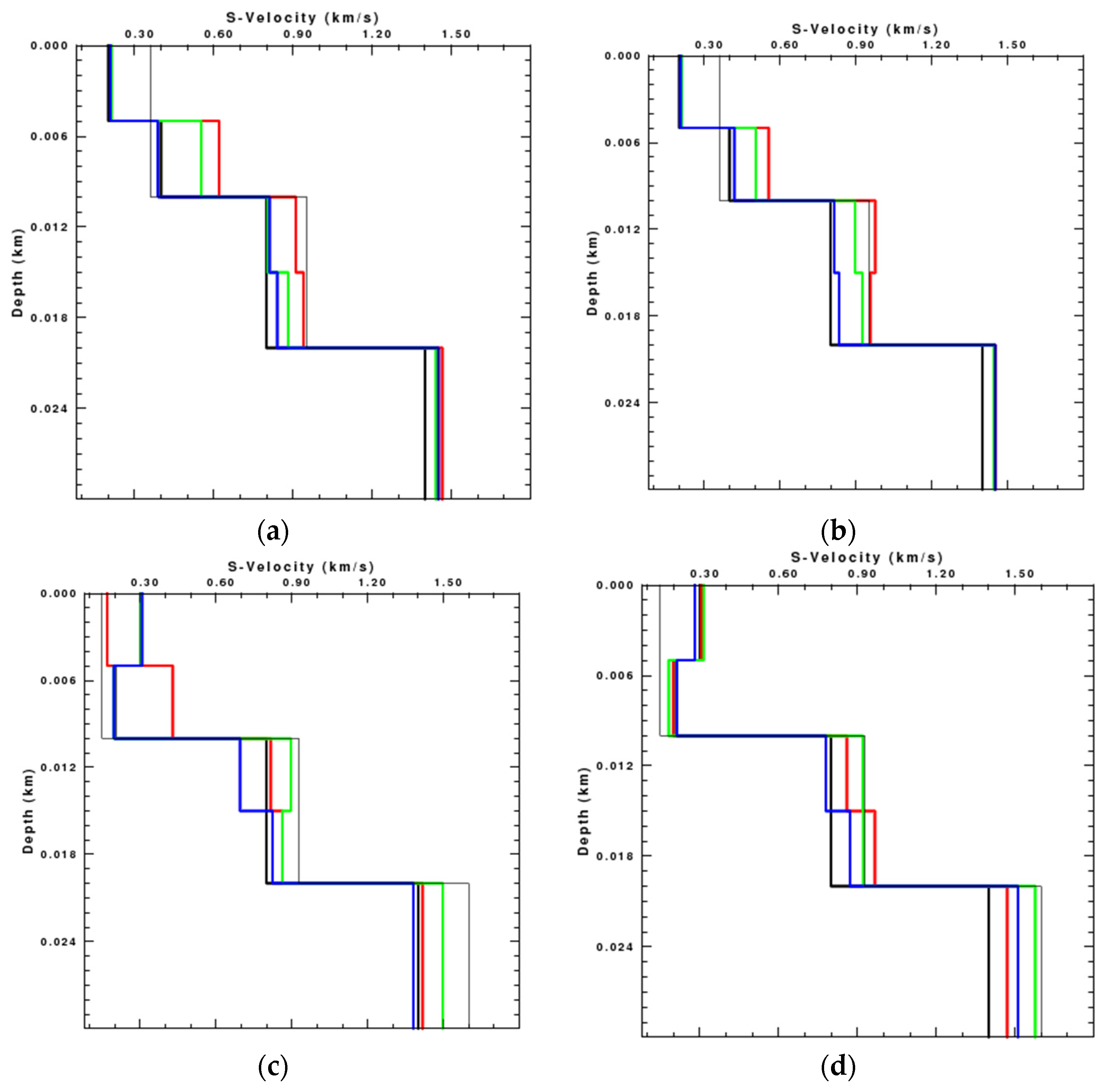
4. Rayleigh Wave Inversion

In order to verify the effect of rotations on the Rayleigh wave inversion, we pick up the phase velocities with the maxima energy from the dispersion spectrum and use the damped least-square inversion method to invert the shear-wave velocity of different models. Because the inversion of Model 3 draws the similar conclusion to that of Model 2 in the middle low-velocity layer, we only display the results of Model 1 and Model 2. The dispersion curves of Model 1 and Model 2 used for inversion are shown in Figure 6, and the comparison of bandwidths among radial, vertical, and rotational data is shown in Table 3.
It is obvious that the dispersion curves on the rotational components are more complete than those on the translational components. The results of the inversion, terminated after 20 iterations, are shown in Figure 7. Limited by space of the paper, we only show the single-component inversion results for clearer comparison, since there are great similarities between the rotational component inversion results and the joint multi-component (radial, vertical, and rotational components) inversion results in the numerical test.
It can be found that the results of the inversion using the rotational component are much better than those using translational components, especially in the deep layer. The S-wave velocity of Model 1 inverted by the rotational component is close to the theoretical model at the depth of 0–5 m and 10–20 m, while that inverted by the translational components has a relatively greater deviation from the theoretical model. In addition, the inversion result using the rotational component almost consists of the theoretical S-wave velocity at the depth of 5–10 m and in the deep layer. The S-wave velocity of Model 2 inverted by the three components approximates the theoretical S-wave velocity within 10 m depth, but is quite different in the deep layer. The inversion results using translational components show a much greater velocity in the deep layer while the inversion using rotational component is close to the theoretical model. The comparison demonstrates that the inversion results using the rotational component are more accurate than those using the translational components.

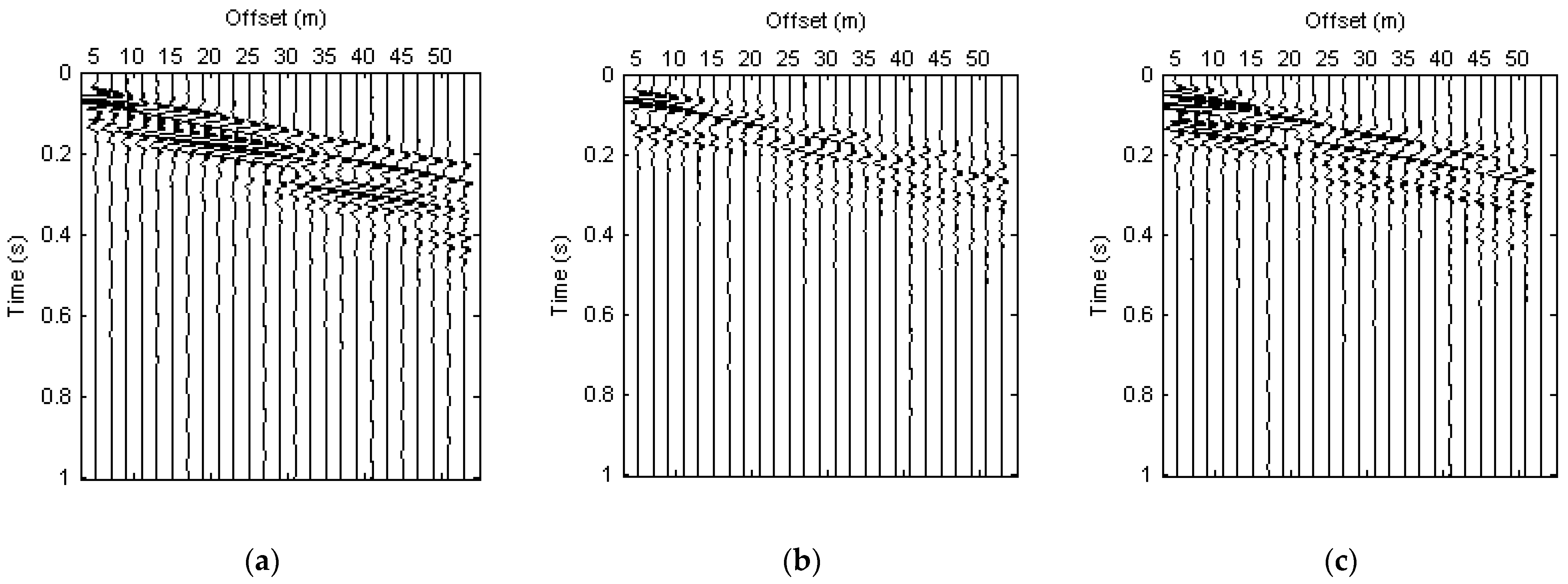
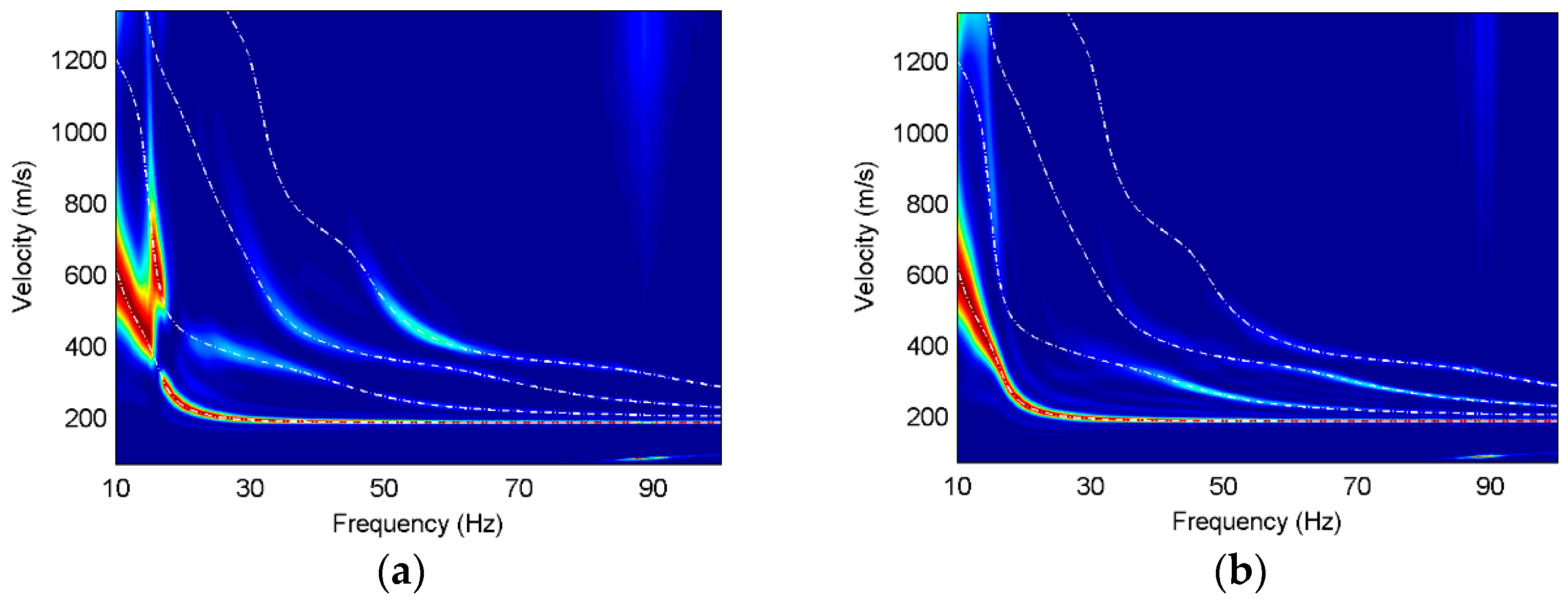
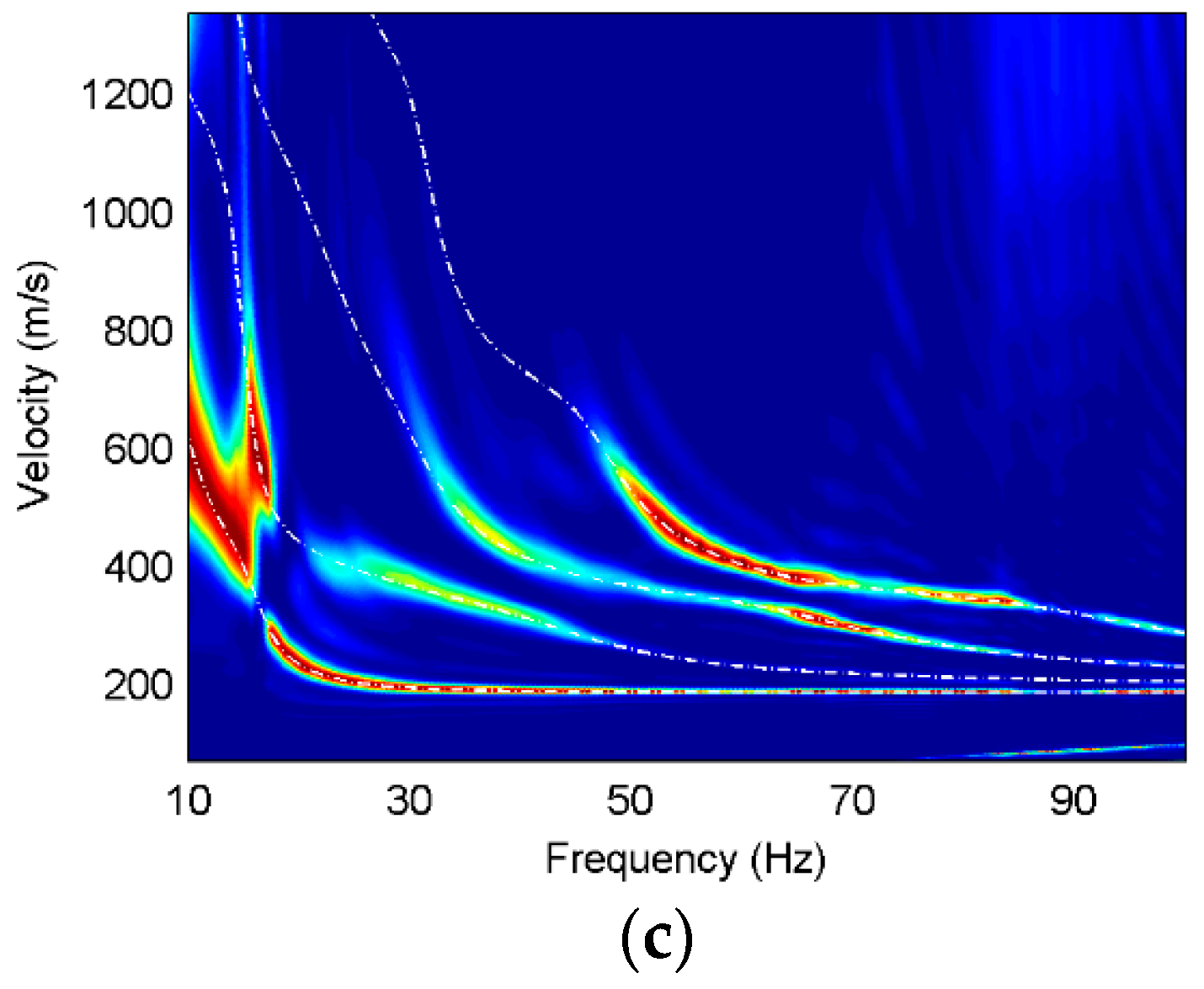
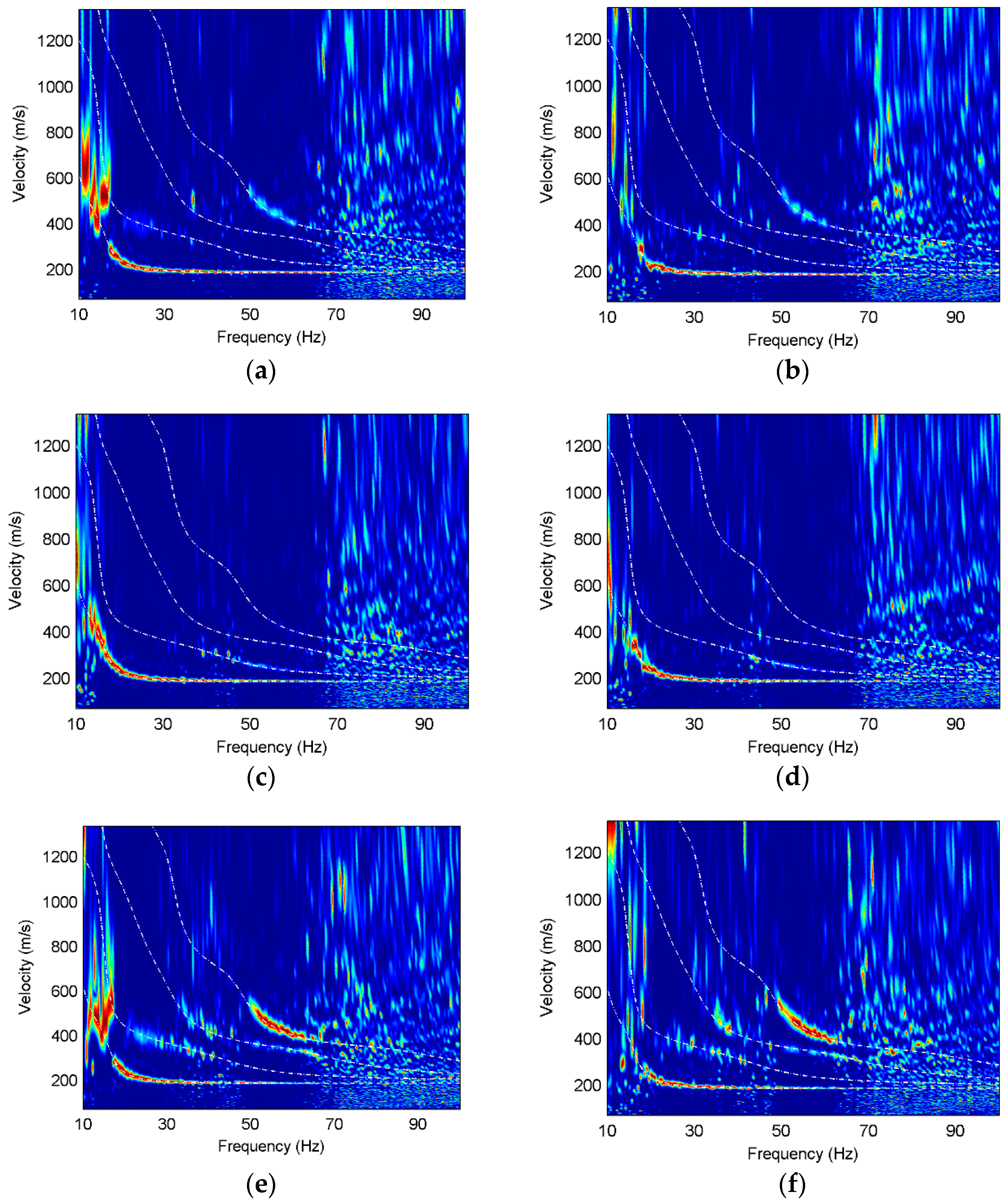
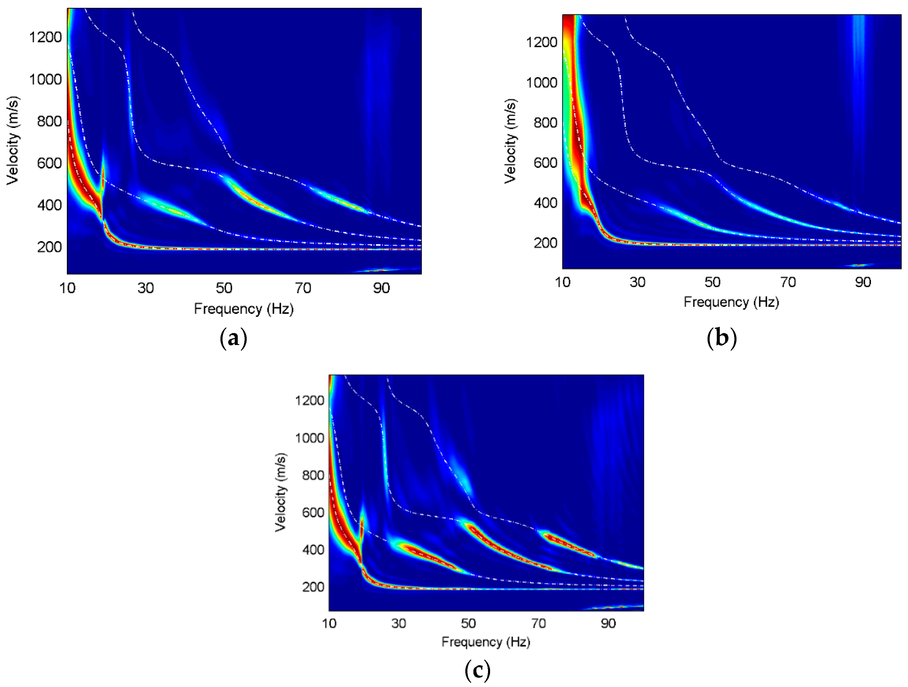
5. Noisy Synthetic Data Test

Considering field applications, we add different level white noises to the seismic data of the Model 1 and Model 2. The signal-to-noise ratio (SNR) is 2.8 and 1.7, respectively. The normalized dispersion images of different components are shown in Figure 8 and Figure 9.
It is obvious that there is only the fundamental-mode energy on the translational component noisy synthetic data of Model 1, and the higher modes are masked by the noise, while the third higher mode is relatively strong on the rotational component, as well as the fundamental mode. Reducing the signal-to-noise ratio has a great influence on the dispersive energy at low frequencies, especially at the frequencies of 10–15 Hz. The fundamental mode on the radial component noisy data of Model 2 is dominant while the higher modes are discontinuous. In contrast, the first and second higher modes on the vertical component have comparative energy and the widest frequency bands since they are less affected by noise. The first higher mode exists at the 20–25 Hz frequencies on the rotational component, but is absent on the translational components. The third higher mode is relatively stronger on the rotational component than that on the other components. This comprehensive comparison illustrates that the Rayleigh waves on the rotational component have stronger anti-noise performance and more complete higher-mode information.
We extract the dispersion curves of different components from the noisy synthetic seismic data and invert the S-wave velocity of Model 1 and Model 2, respectively, as shown in Figure 10:
The S-wave velocity inverted by the radial component is quite different from the theoretical model in the shallow layer, while that inverted by the vertical component has a great deviation from the real model in the deep layer. In contrast, the S-wave velocity inverted by the rotational component is the closest to the theoretical velocity. Reducing the signal-to-noise ratio has a minimal influence on the inversion results with rotation, while increasing the error of the results inverted with the translations.

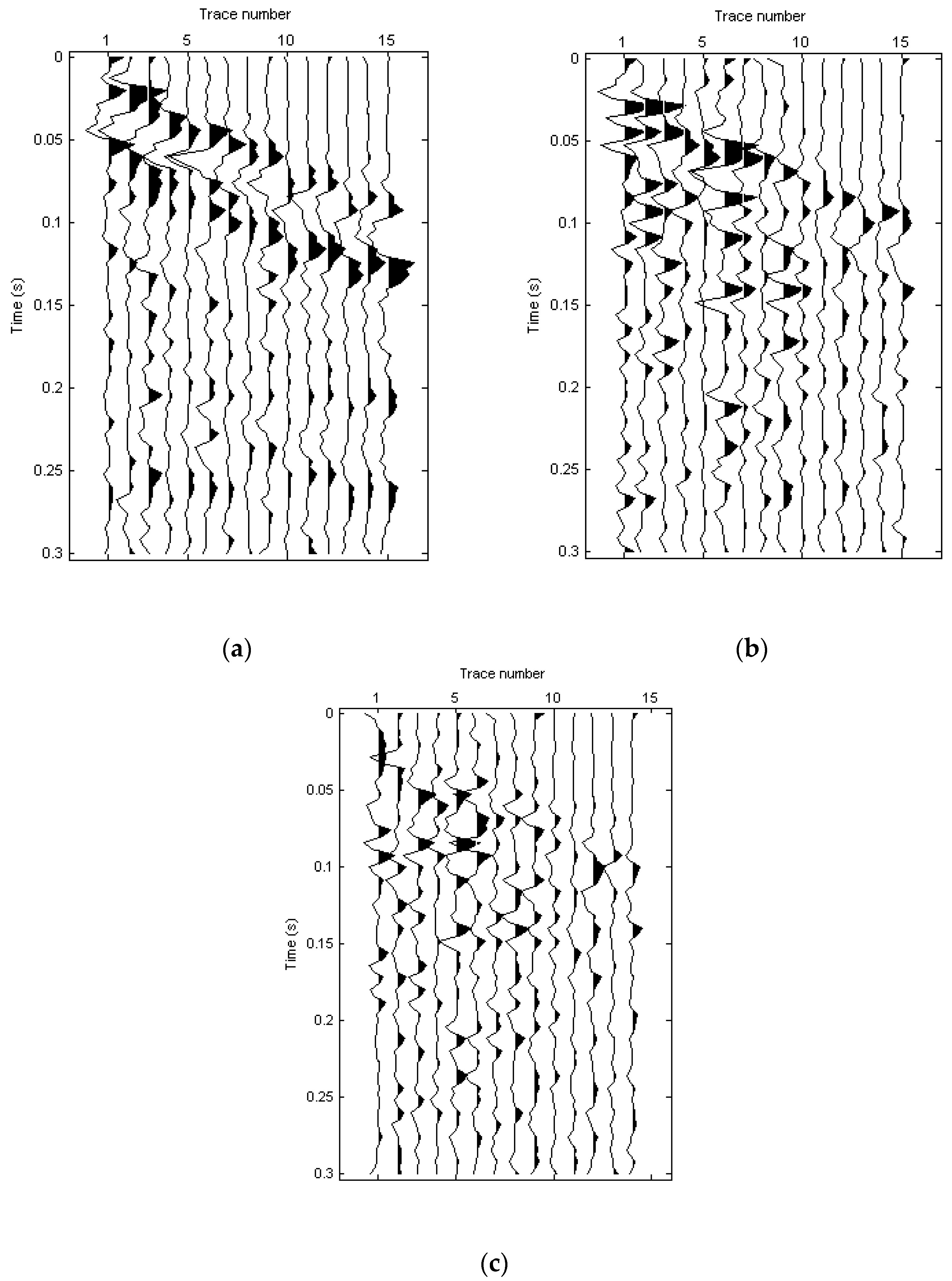
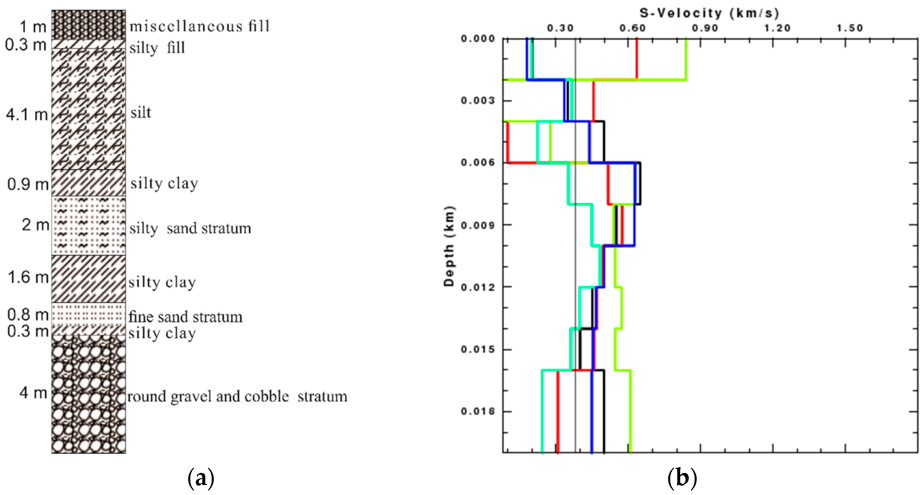
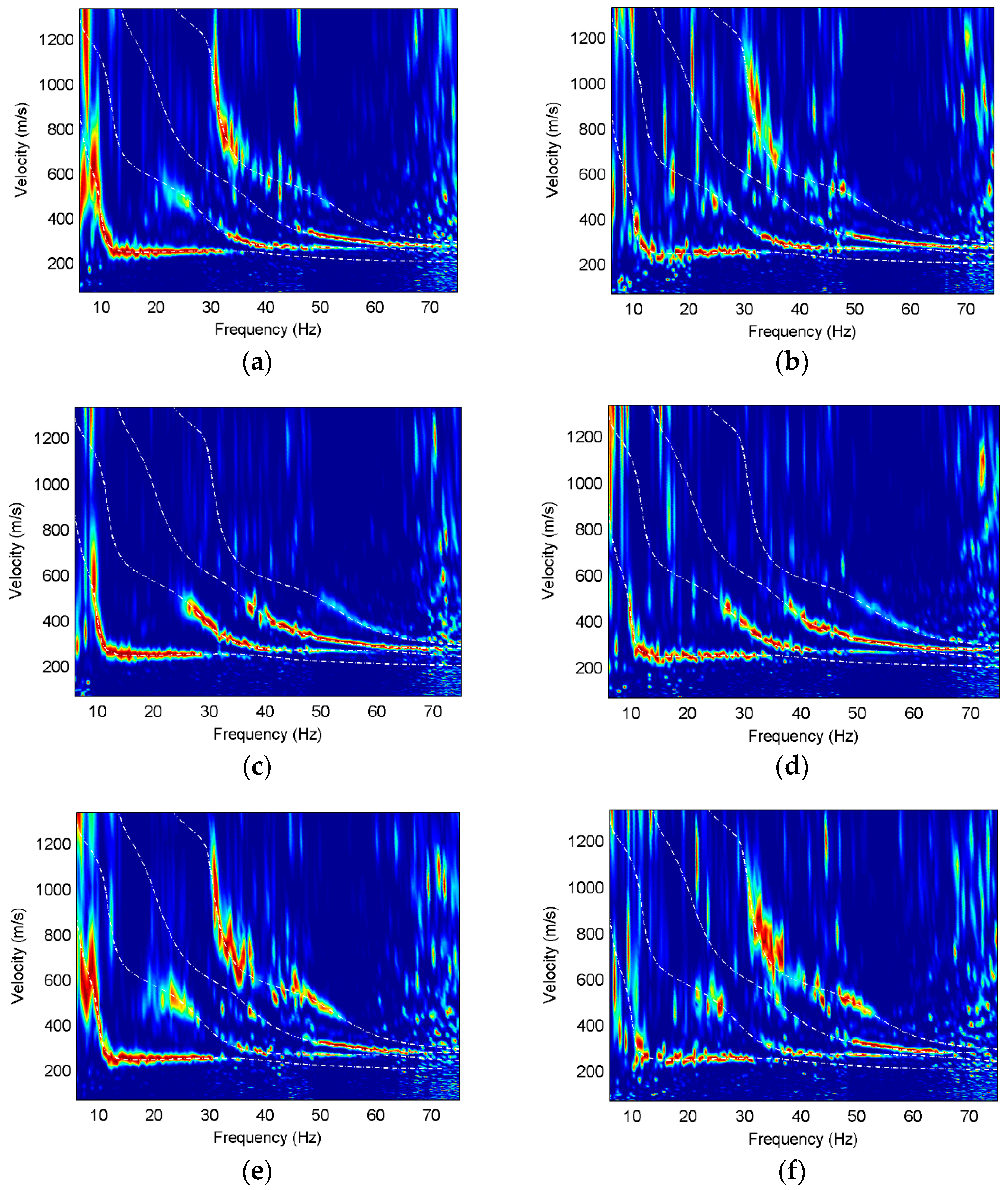
6. Field Seismic Data Test

Wanshousi Station, with a complex underground structure, is a key station of the Beijing No. 16 subway [50]. Beijing Petrosound Geoservices Stock Corp. was entrusted to carry out the two-dimensional three-component seismic observation and to detect the underground structure. They drop an iron hammer onto a solid fixture vertically to excite the seismic waves. There are 81 shots along one line and 15 three-component (3C) geophones with 1 m intervals. The nearest offset is 5 m and the time sample interval is 4 ms. Due to the lack of the rotational observation, we calculate the rotational component Ry with the two-point difference method. The translational and rotational components of the field data are illustrated in Figure 11.
It can be seen that there are obvious surface waves on the three components. The normalized dispersion images of three components are shown in Figure 12.
It can be found that the fundamental mode has strong energy on the translational components, but not all higher modes are present on the three components. The first higher mode is dominant on the radial and rotational components, while the second higher mode and the third higher mode are obviously strong on the vertical component. The fundamental mode and the first higher mode on the rotational component have more low-frequency information while the radial component has richer dispersion information at high frequencies, as shown in Figure 13. Furthermore, the vertical component has higher dispersion modes. It can be demonstrated that the translation and rotation are complementary to each other, and more surface-wave dispersion information can be obtained by jointly using the three components.
There are three shafts in the construction area of Wanshousi station, and the lithologic histogram drawn according to the drilling core is shown in the Figure 14a. Based on the surface-wave dispersion curves in Figure 13, we invert the shallow S-wave velocity structure of 20 m underground by different components respectively, and then jointly use the translational and rotational components to obtain the underground S-wave velocity, as shown in Figure 14b. It can be found that the S-wave velocity inverted by the radial component has a great deviation in the shallow layer, which is the same as that inverted by the vertical component. The S-wave velocity inverted by the rotational component is slightly better than that inverted by the translational components, especially in the shallow layer. It is obvious that the S-wave velocity inverted by the rotational component has a smaller error than that inverted by the translational components, as shown in Table 4. The error of inversion results is calculated by:
E = 1 n i = 1 n e i 2
where E is the error of inversion results, n is the number of the layers, and e i is the error of each layer, which is the deviation from the actual layer velocity.
The error of the S-wave velocity inverted by multi components is the smallest. The inversion results using the translational and rotational components jointly are close to the actual velocity, which shows the significant advantages of the multi-component joint inversion in the soft interlayer identification. It is demonstrated that the joint inversion of the translation and rotation can provide more accurate shear-wave velocity.

7. Discussion and Conclusions

We analyze the Rayleigh wave dispersion characteristics of translational and rotational components for three typical layered engineering models, compare the inversions of different components for synthetic noise-free and noisy data, and perform a test with a subway seismic prospecting case. The synthetic and field examples demonstrate the following:
1. The rotational component has more higher-mode dispersive energy and wider bandwidths than the translational components, particularly richer high-frequency information. The rotational and translational components supplement each other in terms of dispersion curves, which can provide more reliable dispersion information without mode misidentification.
2. The rotational component has stronger anti-noise capability than the translational components. Because there are wider frequency bands and more modes in noisy data, it can improve the inversion accuracy of the shallow shear-wave velocity.
3. The rotation can provide extra dispersion information in practical application. The joint utilization of the translational and rotational components has a considerable improvement on the weak layer identification and shows significant advantages in the shallow inversion.
It is obvious that the rotation is essential for a comprehensive description of the ground motion and that it can provide more accurate underground physical parameters by surface-wave inversion since the additional wave-field information can be obtained. Rotation is beneficial for shallow engineering exploration and surface-wave exploration.
There are still some deficiencies in this paper, since the rotational seismometers are not widely employed in the field observation, and there are non-ignorable differences between the array-derived and observed rotations, especially in the near-earthquake area [51,52]. However, in the future, it is worth popularizing the application of rotational seismometers in shallow seismic engineering and to identify high-precision surface-wave inversion by jointly using the translation and rotation.

Author Contributions

Investigation, X.Q.; Writing—original draft, L.S.; Writing—review & editing, Y.W. All authors have read and agreed to the published version of the manuscript.

Funding

This research was funded by the National Natural Science Foundation of China grant number (U1839208, 62127815). And The APC was funded by the National Natural Science Foundation of China.

Institutional Review Board Statement

Not applicable.

Informed Consent Statement

Not applicable.

Data Availability Statement

Not applicable.

Acknowledgments

We sincerely thank Beijing Petrosound Geoservices Stock Corp. for providing the field data. We greatly acknowledge financial support by the National Natural Science Foundation of China (U1839208, 62127815).

Conflicts of Interest

The authors declare no conflict of interest.

References

  1. Sato, Y. Analysis of dispersed surface waves by means of Frourier transform. Bull. Seismol. Soc. Am. 1955, 33, 33–48. [Google Scholar]
  2. Forsyth, D.W.; Webb, S.C.; Doman, L.M.; Shen, Y. Phase velocities of Rayleigh waves in the MELT experiment on the East Pacific Rise. Science 1998, 280, 1235–1238. [Google Scholar] [CrossRef] [PubMed] [Green Version]
  3. Campillo, M.; Paul, A. Long-range correlations in the diffuse seismic coda. Science 2003, 299, 547–549. [Google Scholar] [CrossRef] [PubMed] [Green Version]
  4. Aki, K. Space and time spectra of stationary stochastic waves, with special reference to microtremors. Bull. Earthq. Res. Inst. 1957, 35, 415–456. [Google Scholar]
  5. Toksoz, M.N.; Lacoss, R.T. Microtremors-mode structure and sources. Science 1968, 159, 872–873. [Google Scholar] [CrossRef] [PubMed]
  6. Ling, S.Q. Research on the Estimation of Phase Velocites of Surface Waves in Microtremors. Ph.D. Thesis, Hokkaido University, Sapporo, Japan, 1994. (In Japanese). [Google Scholar]
  7. Igel, H.; Schreiber, U.; Flaws, A.; Schuberth, B.; Velikoseltsev, A.; Cochard, A. Rotational motions induced by the M8. 1 Tokachi-oki earthquake, September 25, 2003. Geophys. Res. Lett. 2005, 32, L08309. [Google Scholar] [CrossRef] [Green Version]
  8. Kurrle, D.; Igel, H.; Ferreira, A.M.G.; Wassermann, J.; Schreiber, U. Can we estimate local Love wave dispersion properties from collocated amplitude measurements of translations and rotations? Geophys. Res. Lett. 2010, 37, L04307. [Google Scholar] [CrossRef]
  9. Xia, J.; Miller, R.D.; Park, C.B. Estimation of near-surface shear-wave velocity by inversion of Rayleigh waves. Geophysics 1999, 64, 691–700. [Google Scholar] [CrossRef] [Green Version]
  10. Lu, L.; Wang, C.; Zhang, B. Inversion of multimode Rayleigh waves in the presence of a low-velocity layer: Numerical and laboratory study. Geophys. J. Int. 2007, 168, 1235–1246. [Google Scholar] [CrossRef] [Green Version]
  11. Wen, J.C.; Shi, Y.X.; Ning, J.Y. Measurement of high-speed rail surface-wave phase-velocity dispersion. Chin. J. Geophys. 2021, 64, 3246–3256. (In Chinese) [Google Scholar] [CrossRef]
  12. Wang, B.S.; Zeng, X.F.; Song, Z.H.; Li, X.B. Seismic observation and subsurface imaging using an urban telecommunication optic-fiber cable. Chin. Sci. Bull. 2021, 66, 2590–2595. [Google Scholar] [CrossRef]
  13. Tokimatsu, K.; Tamura, S.; Kojima, H. Effects of multiple modes on Rayleigh wave dispersion characteristics. J. Geotech. Eng. 1992, 118, 1529–1543. [Google Scholar] [CrossRef]
  14. Xia, J.H.; Miller, R.D.; Park, C.B.; Tian, G. Inversion of high frequency surface waves with fundamental and higher modes. J. Appl. Geophys. 2003, 52, 45–57. [Google Scholar] [CrossRef]
  15. Feng, S.K.; Sugiyama, T.; Yamanaka, H. Effectiveness of multi-mode surface wave inversion in shallow engineering site investigations. Explor. Geophys. 2005, 36, 26–33. [Google Scholar] [CrossRef]
  16. Pan, L.; Chen, X.F.; Wang, J.N.; Yang, Z.T.; Zhang, D.Z. Sensitivity analysis of dispersion curves of Rayleigh waves with fundamental and higher modes. Geophys. J. Int. 2019, 216, 1276–1303. [Google Scholar] [CrossRef]
  17. Zhou, X.H.; Lin, J.; Zhang, H.Z.; Jiao, J. Mapping extraction dispersion curves of multi-mode Rayleigh waves in microtremors. Chin. J. Geophys. 2014, 57, 2631–2643. (In Chinese) [Google Scholar]
  18. Song, X.; Gu, H.; Liu, J.; Zhang, X. Estimation of shallow subsurface shear-wave velocity by inverting fundamental and higher-mode Rayleigh waves. Soil Dyn. Earthq. Eng. 2007, 27, 599–607. [Google Scholar] [CrossRef]
  19. Mi, B.; Xia, J.; Shen, C.; Wang, L. Dispersion energy analysis of Rayleigh and Love waves in the presence of low-velocity layers in near-surface seismic surveys. Surv. Geophys. 2018, 39, 271–288. [Google Scholar] [CrossRef]
  20. Wang, J.N.; Wu, G.X.; Chen, X.F. Frequency-Bessel transform method for effective imaging of higher-mode Rayleigh dispersion curves from ambient seismic noise data. J. Geophys. Res.—Solid Earth 2019, 124, 3708–3723. [Google Scholar] [CrossRef] [Green Version]
  21. Ikeda, T.; Matsuoka, T.; Tsuji, K.; Hayashi, K. Multimode inversion with amplitude response of surface waves in the spatial autocorrelation method. Geophys. J. Int. 2012, 190, 541–552. [Google Scholar] [CrossRef] [Green Version]
  22. Okada, H.; Suto, K. The Microtremor Survey Method; Society of Exploration Geophysicists: Tulsa, OK, USA, 2003. [Google Scholar]
  23. Zhang, B.X.; Lu, L.Y.; Bao, G.S. A study on zigzag dispersion curves in Rayleigh wave exploration. Chin. J. Geophys. 2002, 45, 263–274. (In Chinese) [Google Scholar] [CrossRef]
  24. Xu, P.F.; Du, Y.N.; Ling, S.Q.; You, Z.W.; Yao, J.; Zhang, H. Microtremor survey method based on inversion of the SPAC coefficient of multi-mode Rayleigh waves and its application. Chin. J. Geophys. 2020, 63, 3857–3867. (In Chinese) [Google Scholar] [CrossRef]
  25. Luo, Y.; Xia, J.; Miller, R.D.; Xu, Y.; Liu, J.; Liu, Q. Rayleighwave dispersive energy imaging using a high-resolution linear radon transform. Pure Appl. Geophys. 2008, 165, 903–922. [Google Scholar] [CrossRef]
  26. Qiu, X.; Wang, Y.; Wang, C. Rayleigh-wave dispersion analysis using complex-vector seismic data. Near Surf. Geophys. 2019, 17, 487–499. [Google Scholar] [CrossRef]
  27. Boaga, J.; Cassiani, G.; Strobbia, C.L.; Vignoli, G. Mode misidentification in Rayleigh waves: Ellipticity as a cause and a cure. Geophysics 2013, 78, 17–28. [Google Scholar] [CrossRef]
  28. Ikeda, T.; Matsuoka, T.; Tsuji, T.; Nakayama, T. Characteristics of the horizontal component of Rayleigh waves in multimode analysis of surface waves. Geophysics 2015, 80, EN1–EN11. [Google Scholar] [CrossRef] [Green Version]
  29. Dal Moro, G.; Ferigo, F. Joint analysis of Rayleigh-and love-wave dispersion: Issues, criteria and improvements. J. Appl. Geophys. 2011, 75, 573–589. [Google Scholar] [CrossRef]
  30. Dal Moro, G.; Moura, R.M.M.; Moustafa, S.S. Multi-component joint analysis of surface waves. J. Appl. Geophys. 2015, 119, 128–138. [Google Scholar] [CrossRef]
  31. Dal Moro, G.; Moustafa, S.S.; Al-Arifi, N.S. Improved holistic analysis of Rayleigh waves for single-and multi-offset data: Joint inversion of Rayleigh-wave particle motion and vertical-and radial-component velocity spectra. Pure Appl. Geophys. 2018, 175, 67–88. [Google Scholar] [CrossRef] [Green Version]
  32. Fichtner, A.; Igel, H. Sensitivity densities for rotational ground-motion measurements. Bull. Seismol. Soc. Am. 2009, 99, 1302–1314. [Google Scholar] [CrossRef]
  33. Sun, L.X.; Wang, Y.; Yang, J.; Zhang, Y.B.; Wang, S.C. Progress in Rotational Seismology. Earth Sci. 2021, 46, 1518–1536. [Google Scholar] [CrossRef]
  34. Kurzych, A.T.; Jaroszewicz, L.R.; Dudek, M.; Kowalski, J.K.; Bernauer, F.; Wassermann, J.; Igel, H. Measurements of Rotational Events Generated by Artificial Explosions and External Excitations Using the Optical Fiber Sensors Network. Sensors 2020, 20, 6107. [Google Scholar] [CrossRef]
  35. Bońkowski, P.A.; Bobra, P.; Zembaty, Z.; Jędraszak, B. Application of Rotation Rate Sensors in Modal and Vibration Analyses of Reinforced Concrete Beams. Sensors 2020, 20, 4711. [Google Scholar] [CrossRef] [PubMed]
  36. Sollberger, D.; Igel, H.; Schmelzbach, C.; Edme, P.; Manen, D.V.; Bernauer, F.; Yuan, S.H.; Wassermann, J.; Schreiber, U.; Robertsson, J.O.A. Seismological Processing of Six Degree-of-Freedom Ground-Motion Data. Sensors 2020, 20, 6904. [Google Scholar] [CrossRef]
  37. Aki, K.; Richardson, P.G. Quantitative Seismology: Theory and Methods; Freeman and Co.: San Francisco, CA, USA, 1980. [Google Scholar]
  38. Aki, K.; Richards, P.G. Quantitative Seismology, 2nd ed.; University Science Book: Herndon, CA, USA, 2002; 700p. [Google Scholar]
  39. Lee, C.E.B.; Celebi, M.; Todorovska, M.I.; Diggles, M.F. Rotational Seismology and Engineering Applications. In Proceedings of the First International Workshop, Menlo Park, CA, USA, 18–19 September 2007; United States Geological Survey: Reston, VA, USA, 2007. [Google Scholar]
  40. Doug, C. The State of Land Seismic. First Break 2018, 36, 65–67. [Google Scholar]
  41. Savazzi, S.; Spagnolini, U.; Goratti, L.; Molteni, D.; Latva-aho, M.; Nicoli, M. Ultra-Wide Band Sensor Networks in Oil and Gas Explorations. IEEE Commun. Mag. 2013, 51, 150–160. [Google Scholar] [CrossRef]
  42. Reddy, V.A.; Stuber, G.L.; Al-Dharrab, S.; Mesbah, W.; Muqaibel, A.H. A Wireless Geophone Network Architecture Using IEEE 802.11af with Power Saving Schemes. IEEE Trans. Wirel. Commun. 2019, 18, 5967–5982. [Google Scholar] [CrossRef]
  43. Barak, O.; Herkenhoff, F.; Dash, R.; Jaiswal, P.; Giles, J.; Ridder, S.; Brune, R.; Ronen, S. Six-component seismic land data acquired with geophones and rotation sensors: Wave-mode selectivity by application of multicomponent polarization filtering. Lead. Edge 2014, 33, 1224–1232. [Google Scholar] [CrossRef]
  44. Cochard, A.; Igel, H.; Schuberth, B.; Suryanto, W.; Velikoseltsev, A.; Schreiber, U.; Wassermann, J.; Scherbaum, F.; Vollmer, D. Rotational Motions in Seismology: Theory, Observation, Simulation. In Earthquake Source Asymmetry, Structural Media and Rotation Effects; Springer: Berlin/Heidelberg, Germany, 2006; pp. 391–411. [Google Scholar]
  45. Herrmann, R.B. Computer Programs in Seismology. Open Files. 2003. Available online: https://www.eas.slu.edu/People/RBHerrmann/CPS330.html (accessed on 15 March 2019).
  46. Herrmann, R.B.; Ammon, C.J. Computer Programs in Seismology—3.30: Surface Waves, Receiver Functions and Crustal Structure. 2002. Available online: www.eas.slu.edu/People/RBHerrmann/CPS330.html (accessed on 15 March 2019).
  47. Sun, L.; Zhang, Z.; Wang, Y. Six-component elastic-wave simulation and analysis. In Proceedings of the EGU General Assembly EGU2018, Vienna, Austria, 4–13 April 2018; Geophysical Research Abstracts, EGU2018-14930-1. Volume 20, p. 14930. [Google Scholar]
  48. Zhang, Z.; Sun, L.X.; Tang, G.B.; Xu, T.; Wang, Y.; Wang, M.L.; Guo, X. Numerical simulation of the six-component elastic-wave field. Chin. J. Geophys. 2020, 63, 2375–2385. [Google Scholar]
  49. Li, D.; Wang, Y.; Sun, L. Calculating Rotational Components of Ground Motions by Finite Difference Method. Earth Sci. 2021, 46, 369–380. [Google Scholar] [CrossRef]
  50. Dong, Z.; Yuan, X.; Yang, B. On construction technique of mechanical holepile methods for subway station of underground excavation. Shanxi Archit. 2017, 43, 171–173. [Google Scholar]
  51. Oliveira, C.S.; Bolt, B.A. Rotational Components of Surface Strong Ground Motion. Earthq. Eng. Struct. Dyn. 1989, 18, 517–526. [Google Scholar] [CrossRef]
  52. Suryanto, W.; Igel, H.; Wassermann, J.; Cochard, A.; Schuberth, B.; Vollmer, D.; Scherbaum, F.; Schreiber, U.; Velikoseltsev, A. First Comparison of Array-Derived Rotational Ground Motions with Direct Ring Laser Measurements. Bull. Seismol. Soc. Am. 2006, 96, 2059–2071. [Google Scholar] [CrossRef] [Green Version]
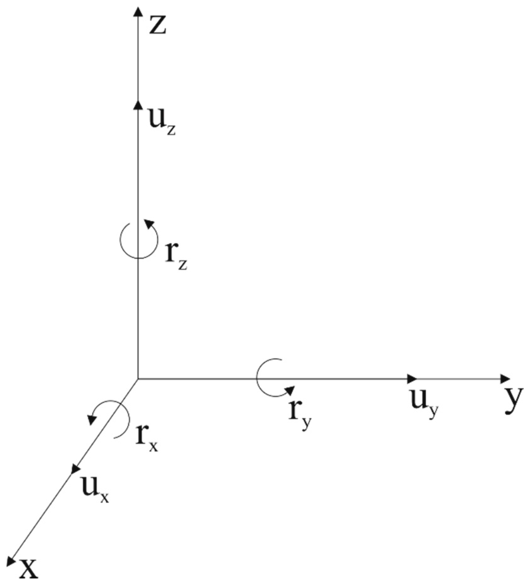
Figure 1. Schematic diagram of the rotational motion.
Sensors 22 00983 g001
Figure 2. Synthetic data for Model 2. (a) X component; (b) Z component; (c) Ry component.
Sensors 22 00983 g002
Figure 3. Dispersion images for Model 1, where the white dashed lines are the theoretical dispersion curves and the red color represents the maximum energy. (a) X component of Model 1; (b) Z component of Model 1; (c) Ry component of Model 1.
Sensors 22 00983 g003aSensors 22 00983 g003b
Figure 4. Dispersion images for Model 2, where the white dashed lines are the theoretical dispersion curves and the red color represents the maximum energy. (a) X component of Model 2; (b) Z component of Model 2; (c) Ry component of Model 2.
Sensors 22 00983 g004
Figure 5. Dispersion images for Model 3, where the white dashed lines are the theoretical dispersion curves and the red color represents the maximum energy. (a) X component of Model 3; (b) Z component of Model 3; (c) Ry component of Model 3.
Sensors 22 00983 g005
Figure 6. Dispersion curves for Model 1 and Model 2, where the black lines are the theoretical dispersion curves and different shapes of points correspond to the different modes. (a) X component of Model 1; (b) X component of Model 2; (c) Z component of Model 1; (d) Z component of Model 2; (e) Ry component of Model 1; (f) Ry component of Model 2.
Sensors 22 00983 g006
Figure 7. Results of the Rayleigh wave inversion using the radial (red line), vertical (green line), and rotational (blue line) seismic data respectively. The black thick line is the theoretical S-wave velocity, and the black thin line is the initial S-wave velocity. (a) Model 1; (b) Model 2.
Sensors 22 00983 g007
Figure 8. Dispersion images of noisy data of Model 1, where the white dashed lines are the theoretical dispersion curves and the red color represents the maximum energy. SNR of the left column is 2.8 and SNR of the right column is 1.7. (a) X component; (b) X component; (c) Z component; (d) Z component; (e) Ry component; (f) Ry component.
Sensors 22 00983 g008
Figure 9. Dispersion images of noisy data of Model 2, where the white dashed lines are the theoretical dispersion curves and the red color represents the maximum energy. SNR of the left column is 2.8 and SNR of the right column is 1.7. (a) X component; (b) X component; (c) Z component; (d) Z component; (e) Ry component; (f) Ry component.
Sensors 22 00983 g009
Figure 10. Inversion results of the noisy data using the radial (red line), vertical (green line), and rotational (blue line) components, respectively. The black thick line is the theoretical S-wave velocity and the black thin line is the initial S-wave velocity. SNR of the left column is 2.8 and SNR of the right column is 1.7. (a) Model 1; (b) Model 1; (c) Model 2; (d) Model 2.
Sensors 22 00983 g010
Figure 11. Field seismic data. (a) X; (b) Z; (c) Ry.
Sensors 22 00983 g011
Figure 12. Normalized dispersion images of the field data, where the red color represents the maximum energy. (a) X; (b) Z; (c) Ry.
Sensors 22 00983 g012
Figure 13. Comparison of dispersion curves extracted from different components.
Sensors 22 00983 g013
Figure 14. Field data test: (a) the lithologic histogram; (b) inversion results using the radial (red line), vertical (yellow line), rotational (green line), and multi-component (blue line) seismic data, respectively. The black thick line is the actual S-wave velocity, and the black thin line is the initial S-wave velocity.
Sensors 22 00983 g014
Table 1. The ground motion.
AxisTranslation Rotation
xRadialuxRollrx
yTransverseuy Pitchry
zVerticaluz Yawrz
Table 2. The model parameters.
Model 1Model 2Model 3
ThicknessVpVsDenVpVsDenVpVsDen
56002001800110030018506002001800
512004001900600200180018008002000
10180080020001800800200013006001950
-290014002100290014002100290014002100
Thickness, (m); Vp, the velocity of P-waves (m/s); Vs, the velocity of S-waves (m/s); Den, density (kg/m3).
Table 3. Comparison of bandwidths among the radial, vertical and rotational data.
ComponentFundamental
Mode (Hz)
First Higher
Mode (Hz)
Second Higher
Mode (Hz)
Third Higher
Mode (Hz)
Model 1radial10–15, 18–10012–15-50–58
vertical10–10044–5068–72-
rotational10–15, 18–10012–15, 22–4232–42, 60–8448–86, 92–100
Model 2radial8–3232–5444–7530–36
vertical8–3226–5436–75-
rotational8–3222–28, 32–5444–7528–52
Table 4. Error of the inversion results using the radial (X), vertical (Z), rotational (Ry), and multi-component (X + Z + Ry) seismic data.
Depth (m)XZRyX + Z + Ry
e i 0~20.435 0.638 −0.001 −0.021
2~40.105 −0.301 0.016 0.005
4~6−0.401 −0.224 −0.278 −0.061
6~8−0.135 −0.022 −0.299 −0.023
8~100.024 −0.012 −0.103 0.075
10~12−0.005 0.045 −0.019 −0.002
12~140.020 0.122 −0.053 0.016
14~160.058 0.146 −0.040 0.053
-−0.193 0.108 −0.257 −0.052
E -0.205 0.245 0.158 0.040
Publisher’s Note: MDPI stays neutral with regard to jurisdictional claims in published maps and institutional affiliations.

