
Baseline Correction of Acceleration Data Based on a Hybrid EMD–DNN Method

Abstract
:1. Introduction
- (1)
- The ground rotates or tilts [4];
- (2)
- The recorded data is mixed with low-frequency noise from environmental vibration or the vibration of the instrument itself;
- (3)
- The assumed initial value of velocity or displacement is inconsistent with the actual situation;
- (4)
- Data processing errors and transducer hysteresis [5].
- (1)
- (2)
- (3)
- Eliminate drift error by eliminating velocity and displacement polynomial trend.
- (1)
- Some methods rely on subjective experience judgment, and the uncertainty of correction is large;
- (2)
- The process of some methods is complicated, and the calculation efficiency is low. The summary comparison of these methods is shown in Table 1.
2. Traditional Baseline Correction Method
- (1)
- The quadratic value of acceleration is ;
- (2)
- The least squares method is used to fit the linear error trend of ;
- (3)
- The final actual displacement is obtained.
3. Baseline Correction Method Based on EMD–DNN
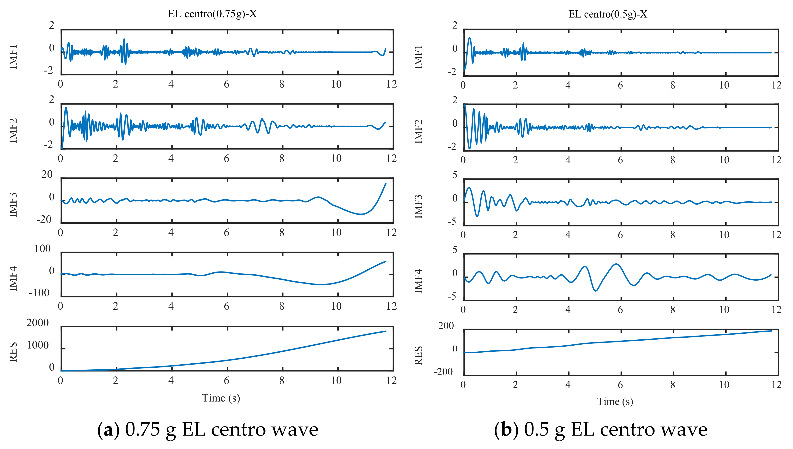
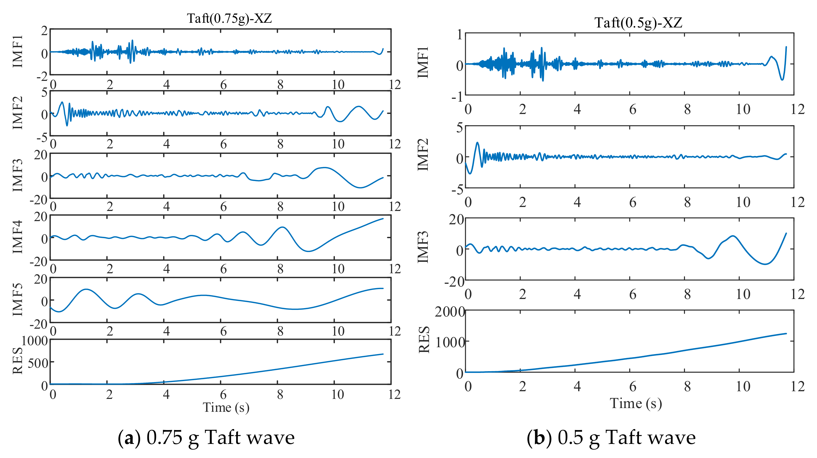
3.1. EMD
- (1)
- In the whole time series, the number of extreme points is equal to the number of zero crossings or the difference is, at most, 1.
- (2)
- At any point, the average of upper and lower envelopes is 0. The EMD process is implemented through a process called “screening”. Its specific treatment methods are as follows:
- (1)
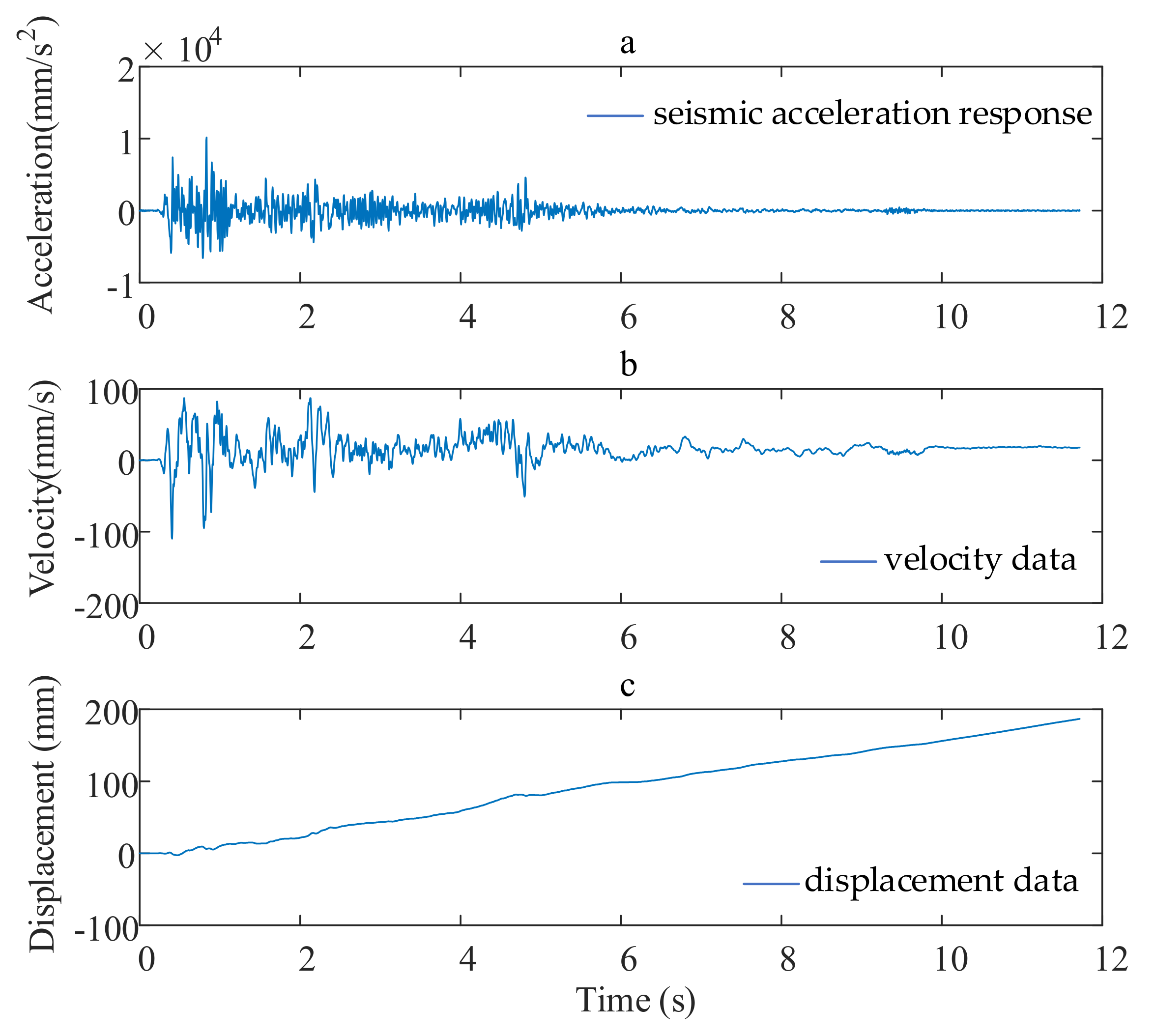
- The pseudo velocity can be obtained by the acceleration record integration.
- (2)
- Each IMF and trend term can be obtained through the empirical mode decomposition of pseudo velocity . The correction velocity is obtained by removing the trend term and reconstructing the IMF component.
- (3)
- The pseudo displacement is obtained by velocity integration.
- (4)
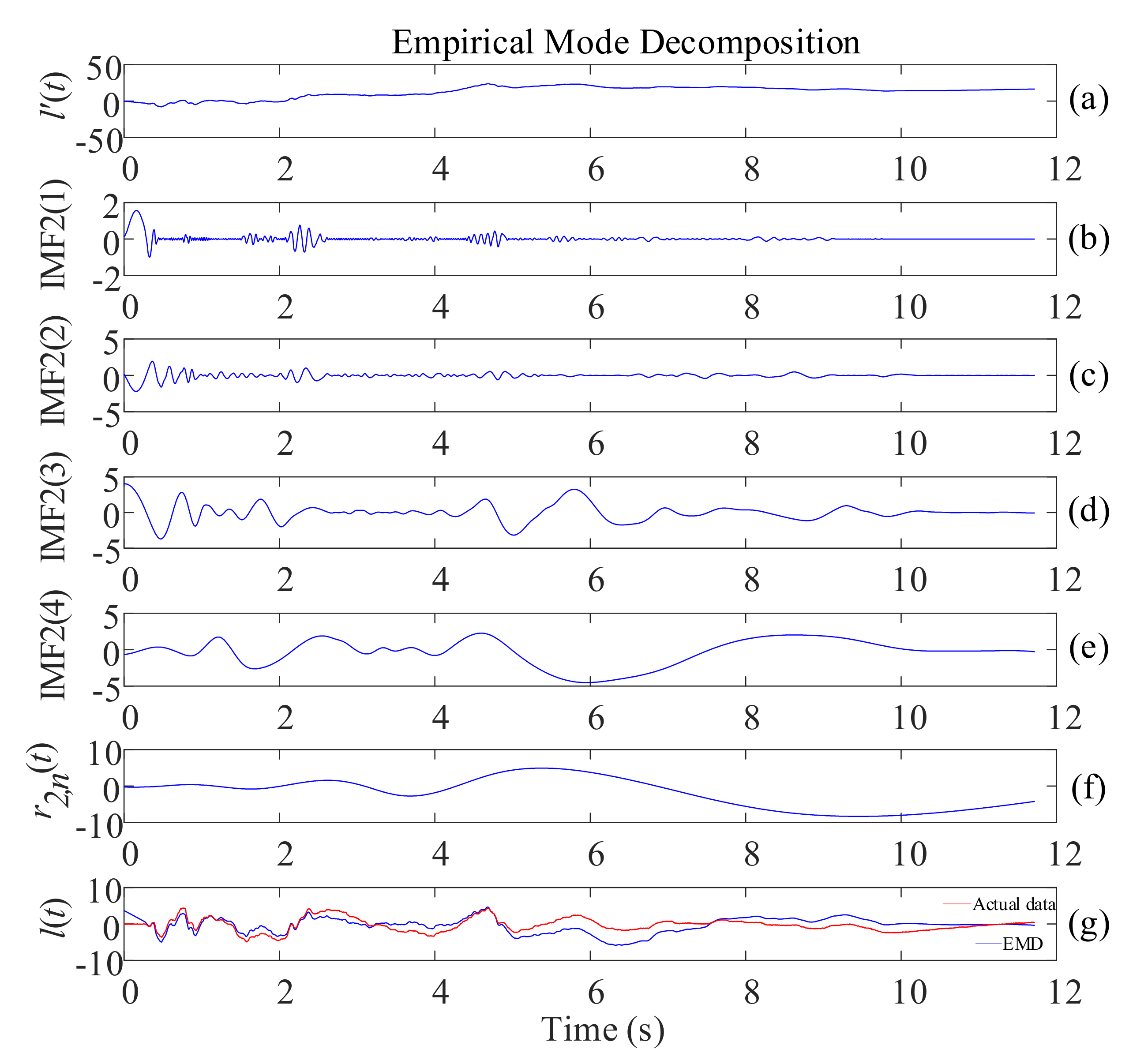
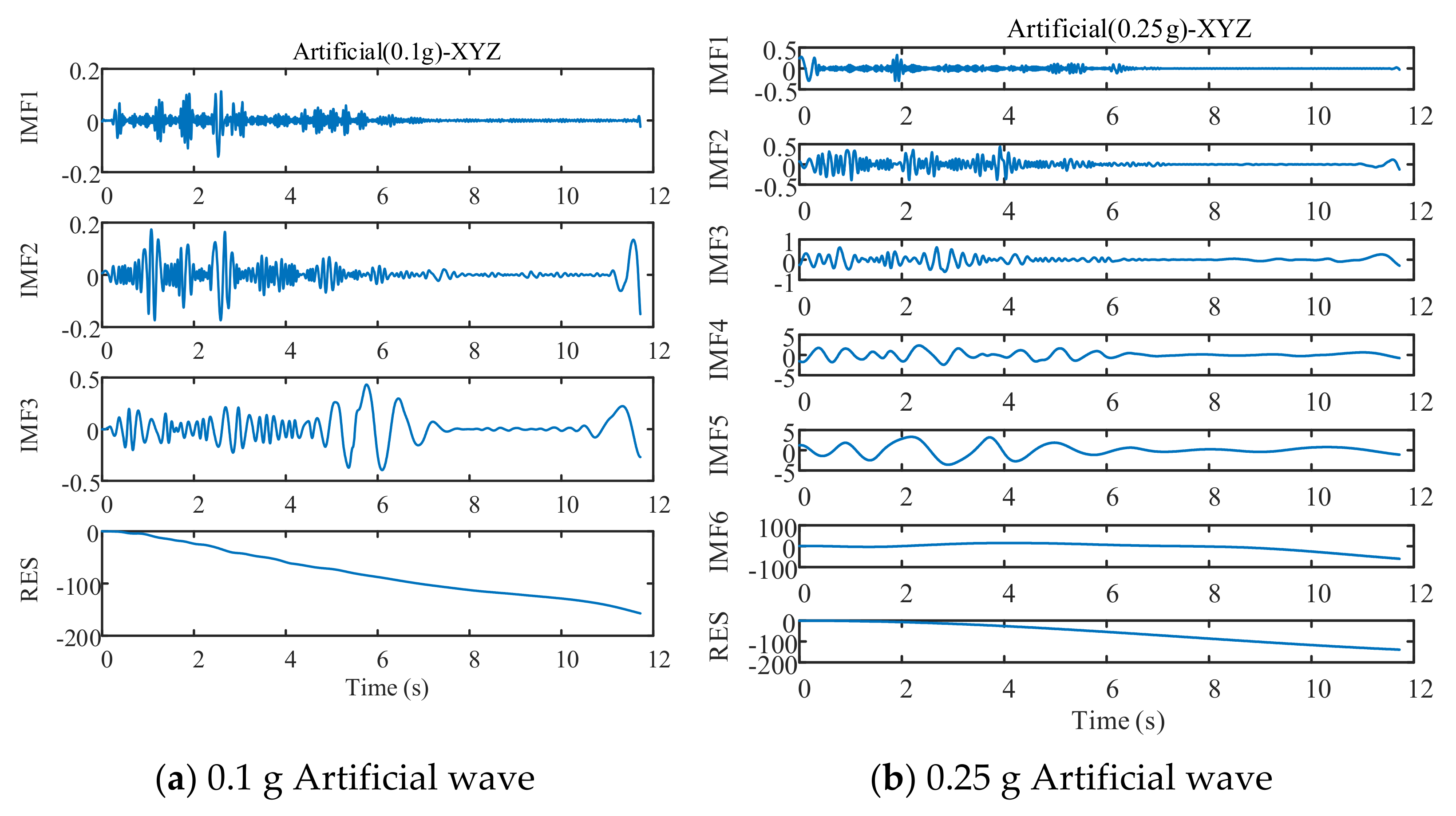
- The pseudo displacement is decomposed by the EMD to obtain each and the trend term (Figure 2). The trending term is removed, and the correction displacement is obtained by reconstructing the components. The formula is as follows:
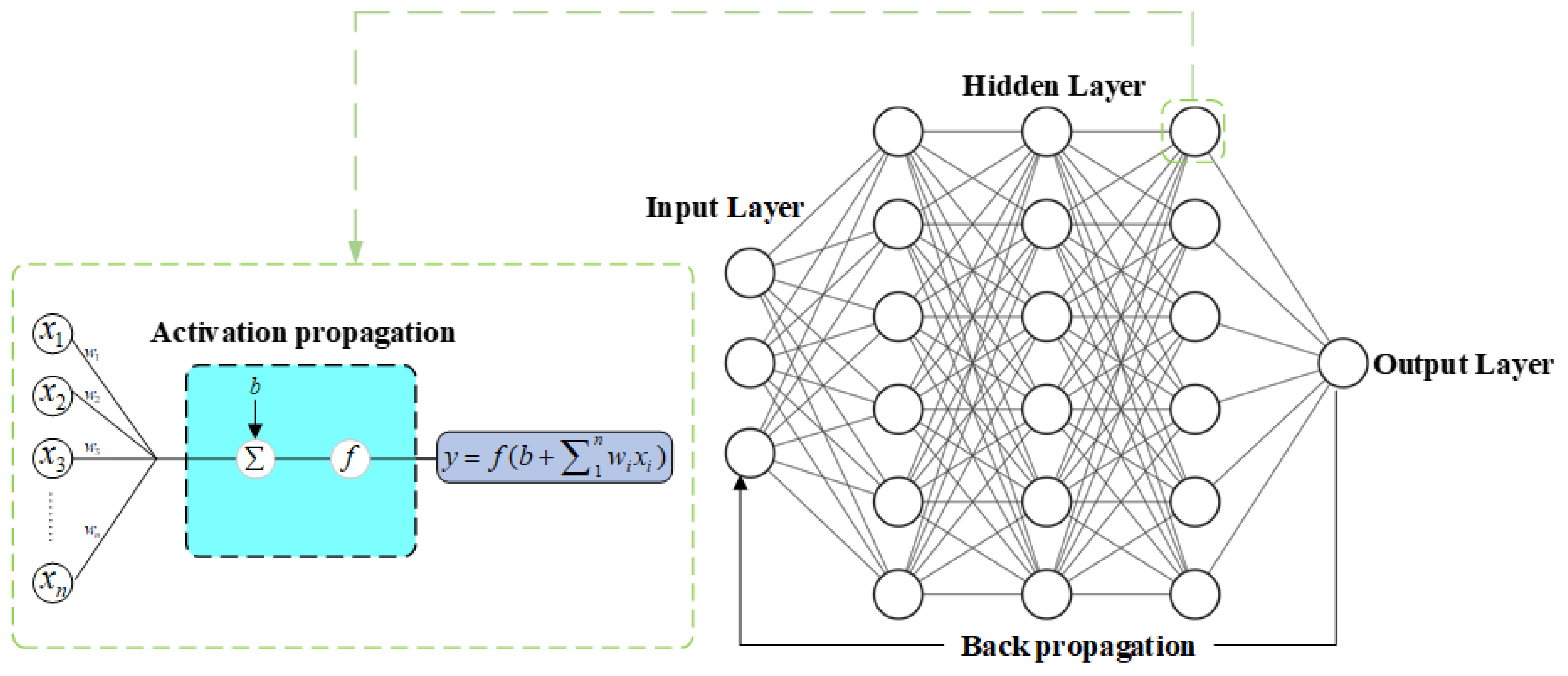
3.2. DNN
3.3. EMD–DNN
- (1)
- The drift displacement time history was obtained by quadratic numerical integration of the original acceleration time history;
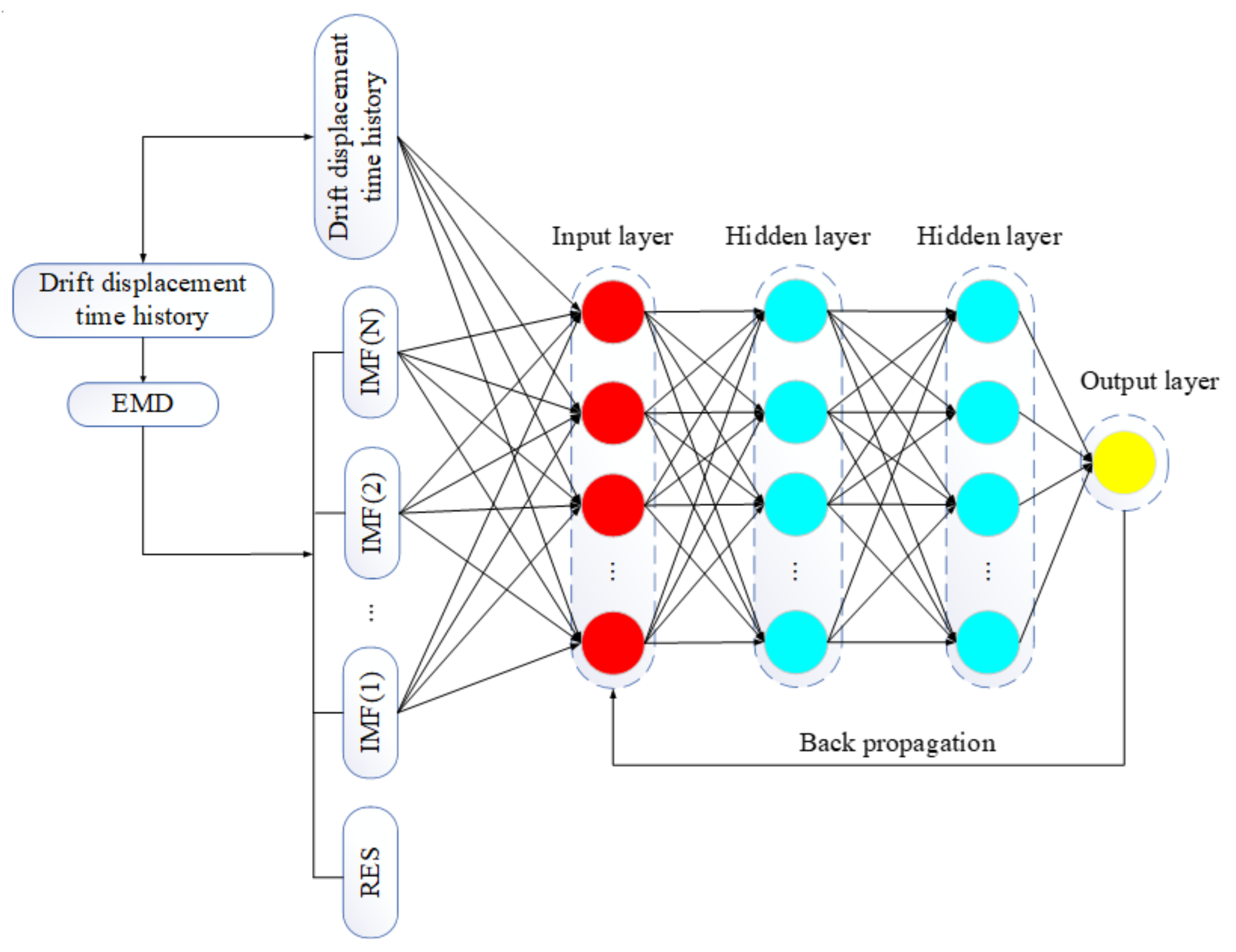
- (2)
- Drift displacement time history was divided into a training set and testing set. The training set and testing set were, respectively, decomposed into multiple IMF components and residual RES by EMD. IMF component and drift displacement time history of the training set were taken as a feature set to form a combined data set , and the testing set was the combined data set .
- (3)
- The combined data set was input into the DNN model as the input layer. The predicted value was obtained through forward propagation. The loss value was obtained by combining the predicted value with the actual displacement record and acted on the DNN model through back propagation to optimize the model. Finally, the combined data set was input into the optimal model to evaluate the predicted results. The specific EMD–DNN correction process is shown in Figure 4.
4. Experimental Verifications
4.1. Experiment Introduction
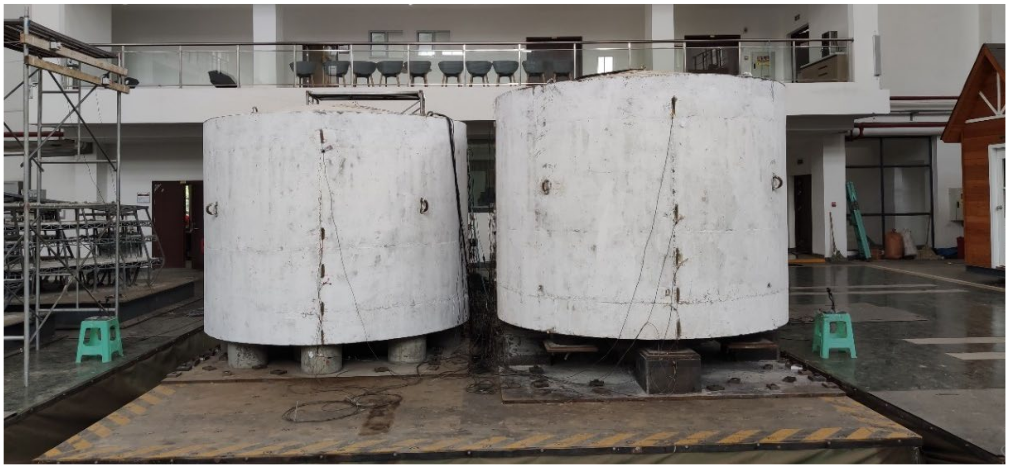
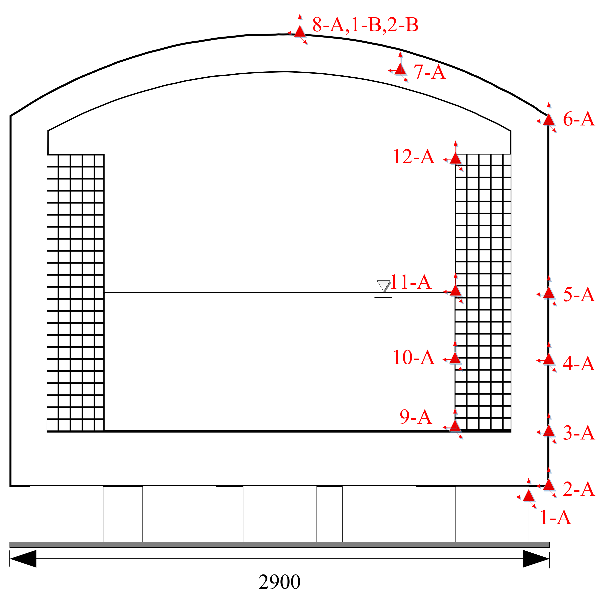
4.1.1. Sensor Arrangement
- (1)
- Acceleration sensor layout
- 1.
- Pile: one acceleration sensor was arranged in each X, Y, and Z direction of the pile head of the isolation tank and the nonisolation tank.
- 2.
- Inner tank: there were four measuring points along the height direction, respectively, in the isolation tank and the nonisolation tank, and one acceleration sensor was arranged at each measuring point in X, Y, and Z directions, respectively.
- 3.
- The outer tank: there were seven measuring points on the tank body and its dome (there were two measuring points on the dome and five measuring points on the tank body along the height direction). One acceleration sensor was arranged on each measuring point in the X, Y, and Z directions, respectively.
- (2)
- Displacement meter layout
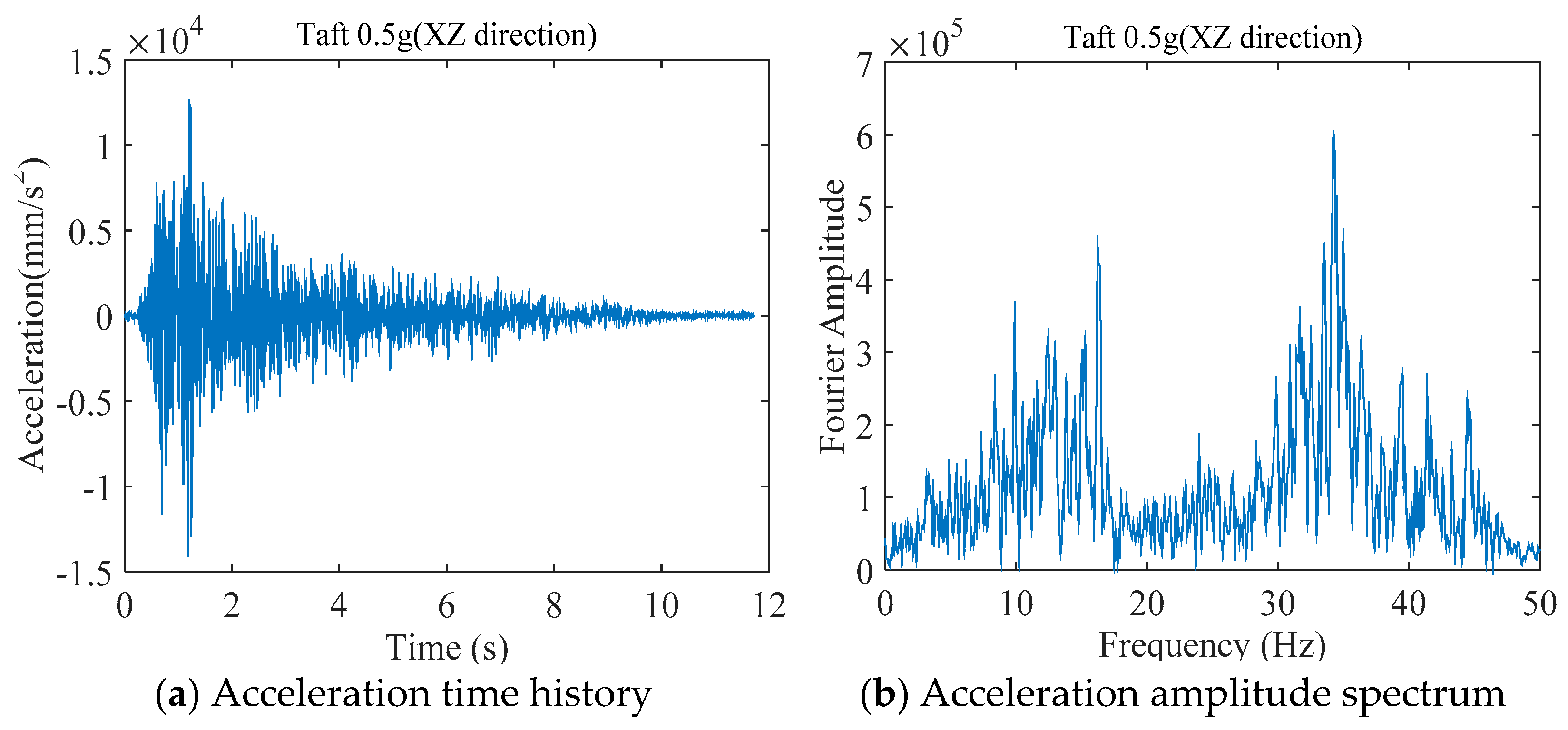
4.1.2. Select Wave Type and Parameter Settings
4.1.3. The Evaluation Index
- (1)
- Mean absolute error (MAE) [25]
- (2)
- Mean square error (MSE) [26]
- (3)
- Root mean square error (RMSE) [27]
- (4)
- R-square [28]where is the actual displacement data, is the average values of the actual displacement data, and is the corrected data.
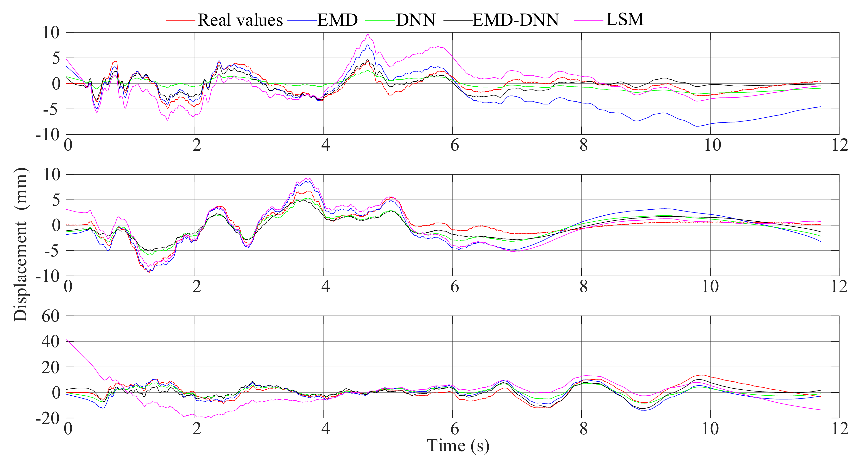
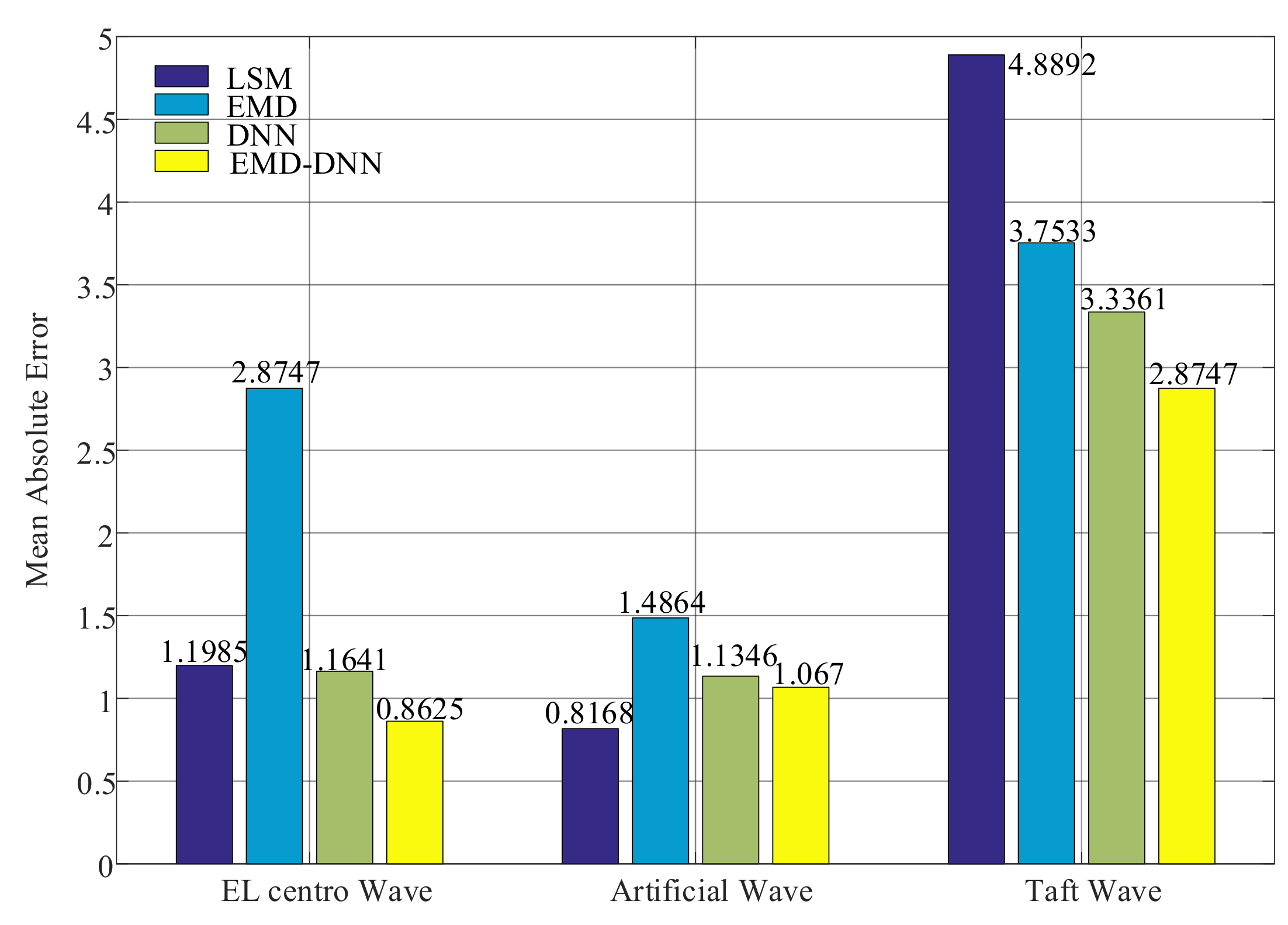
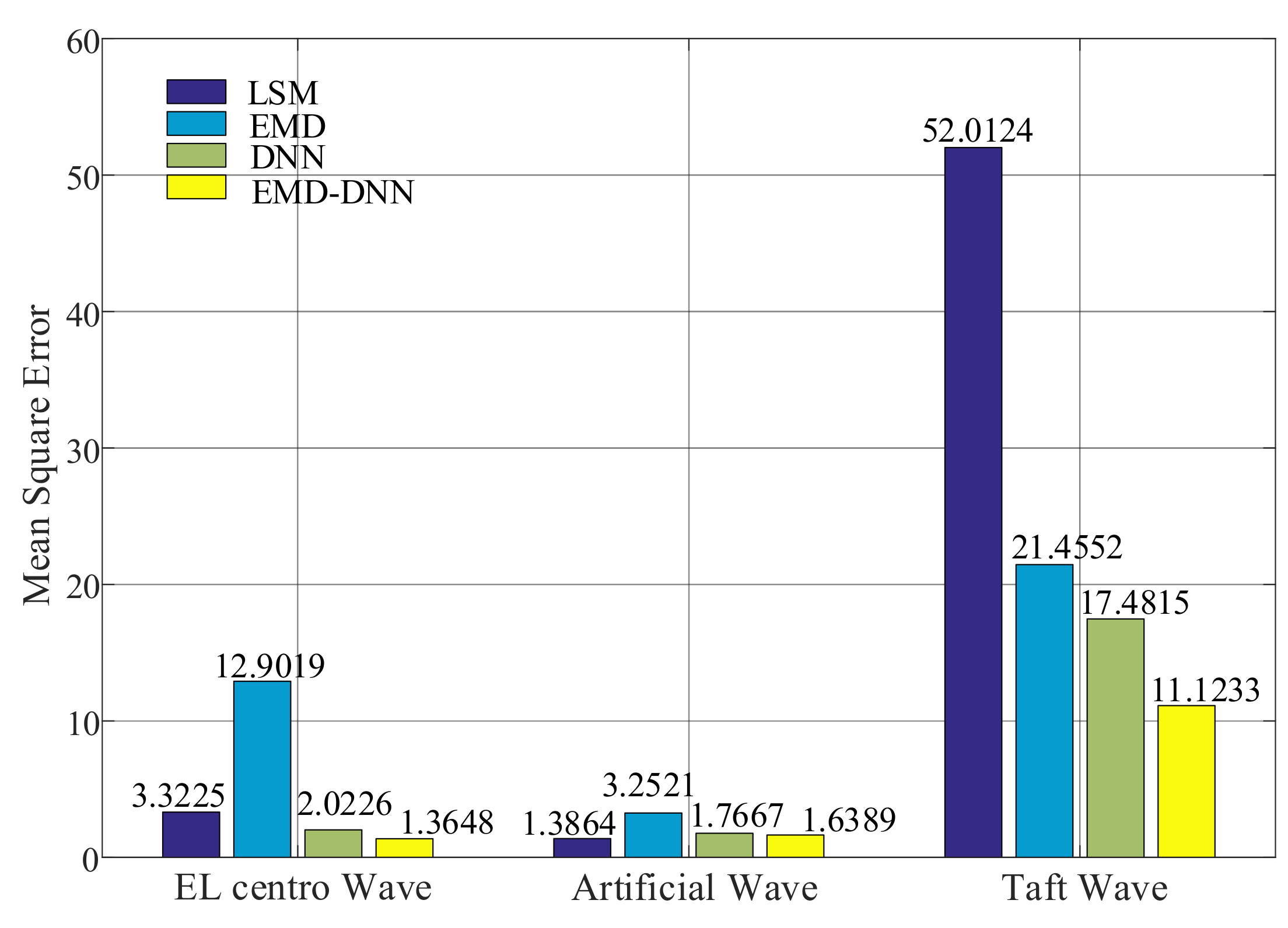
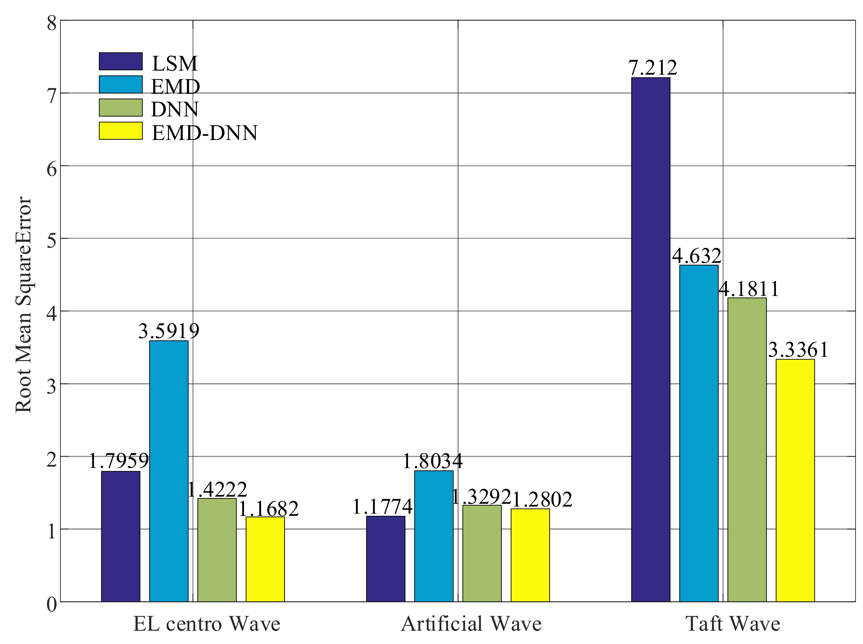
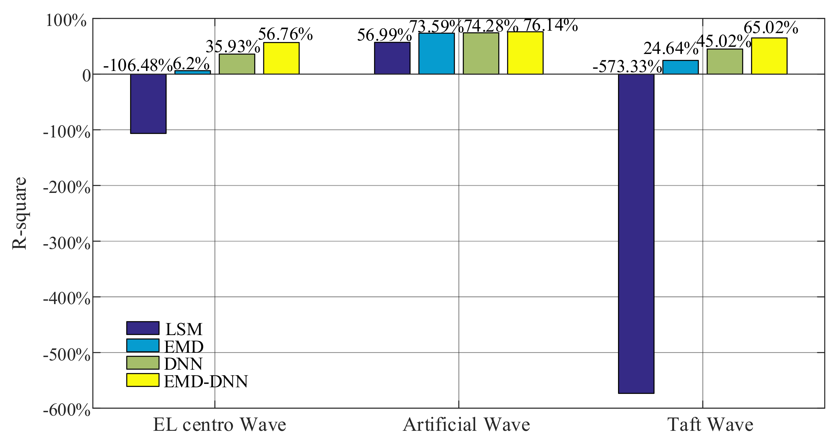
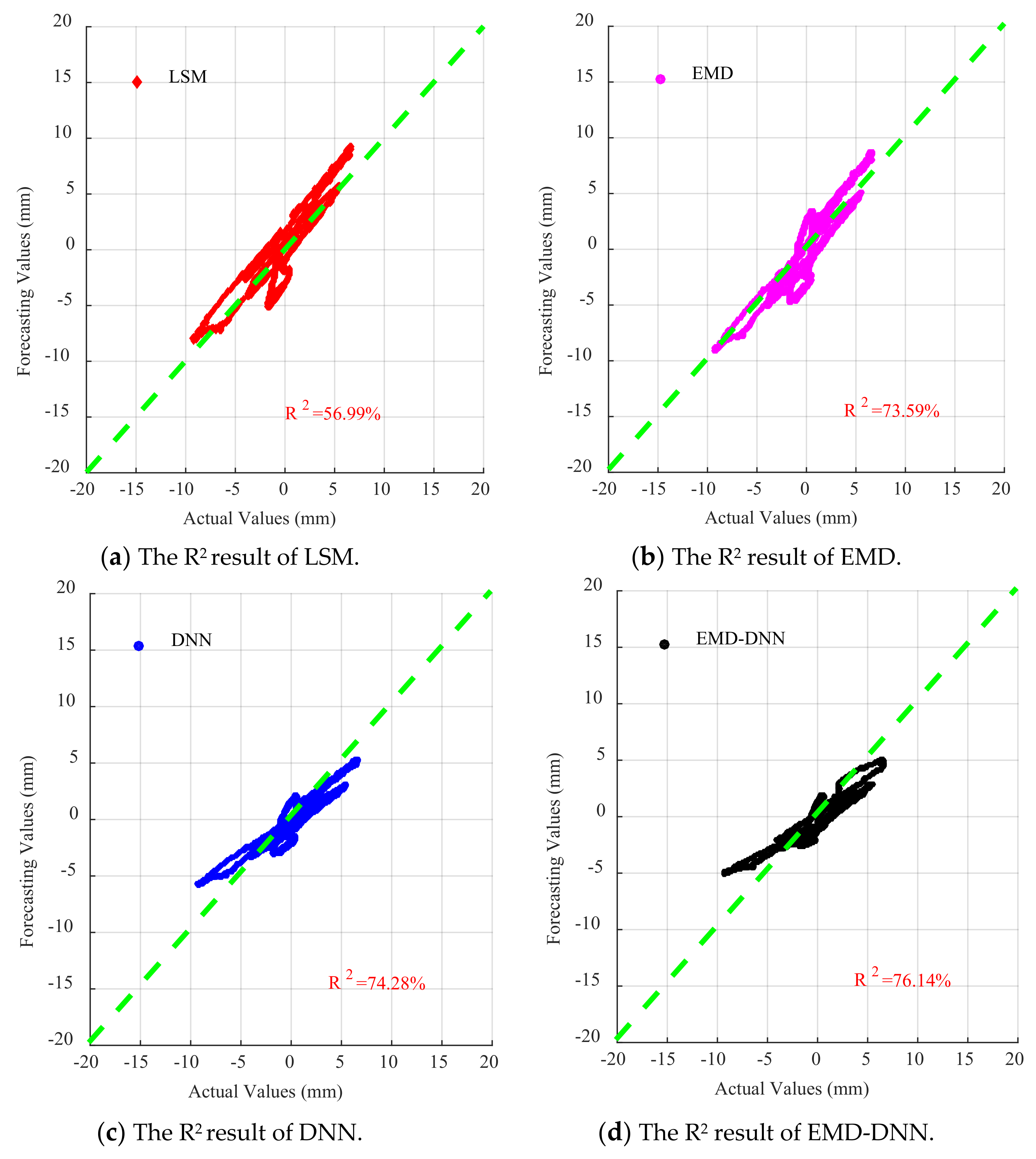
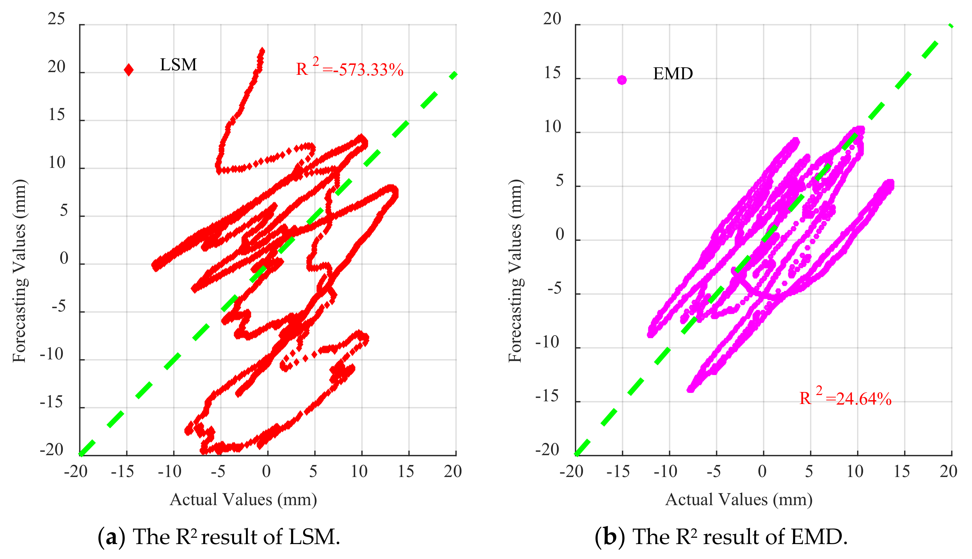
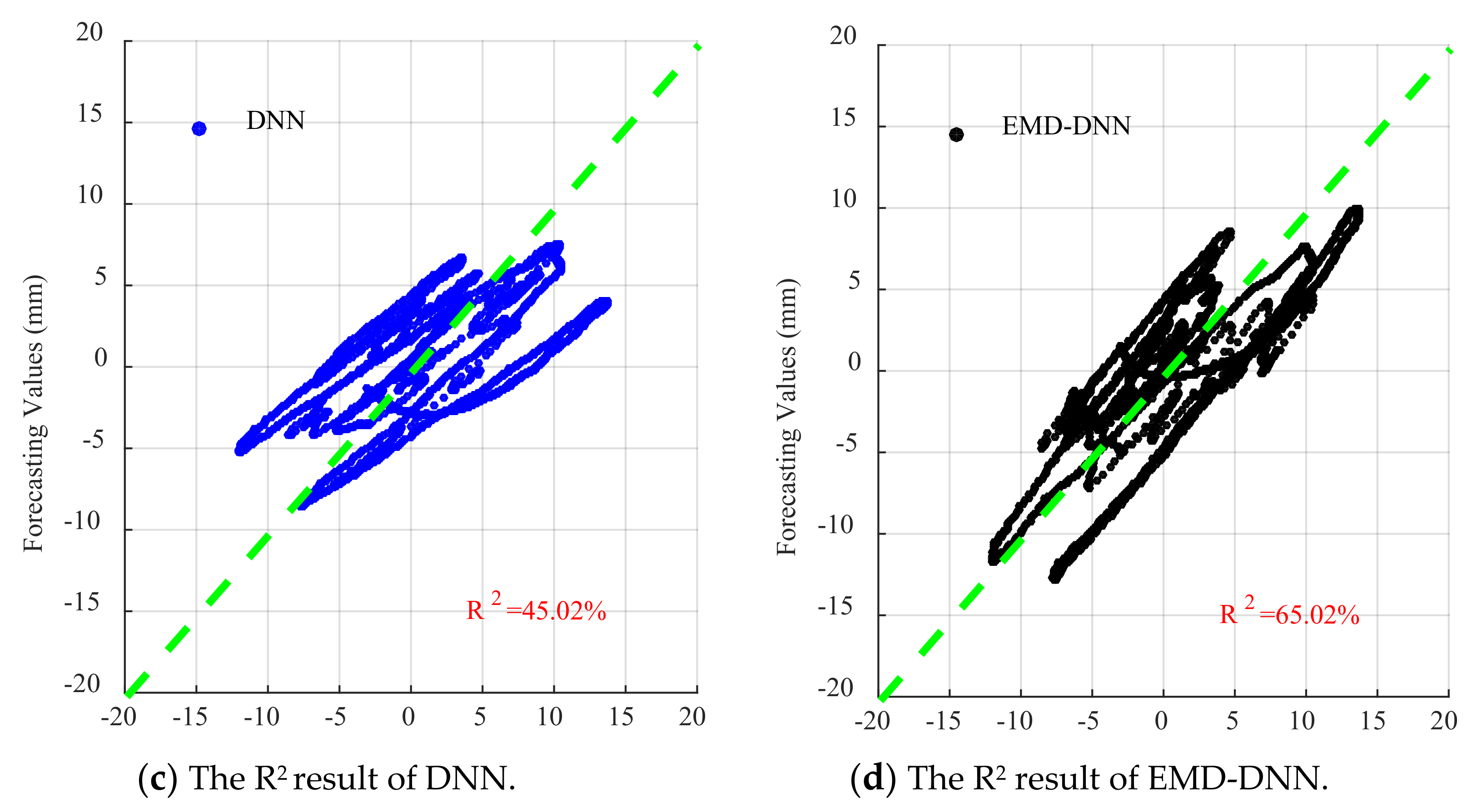
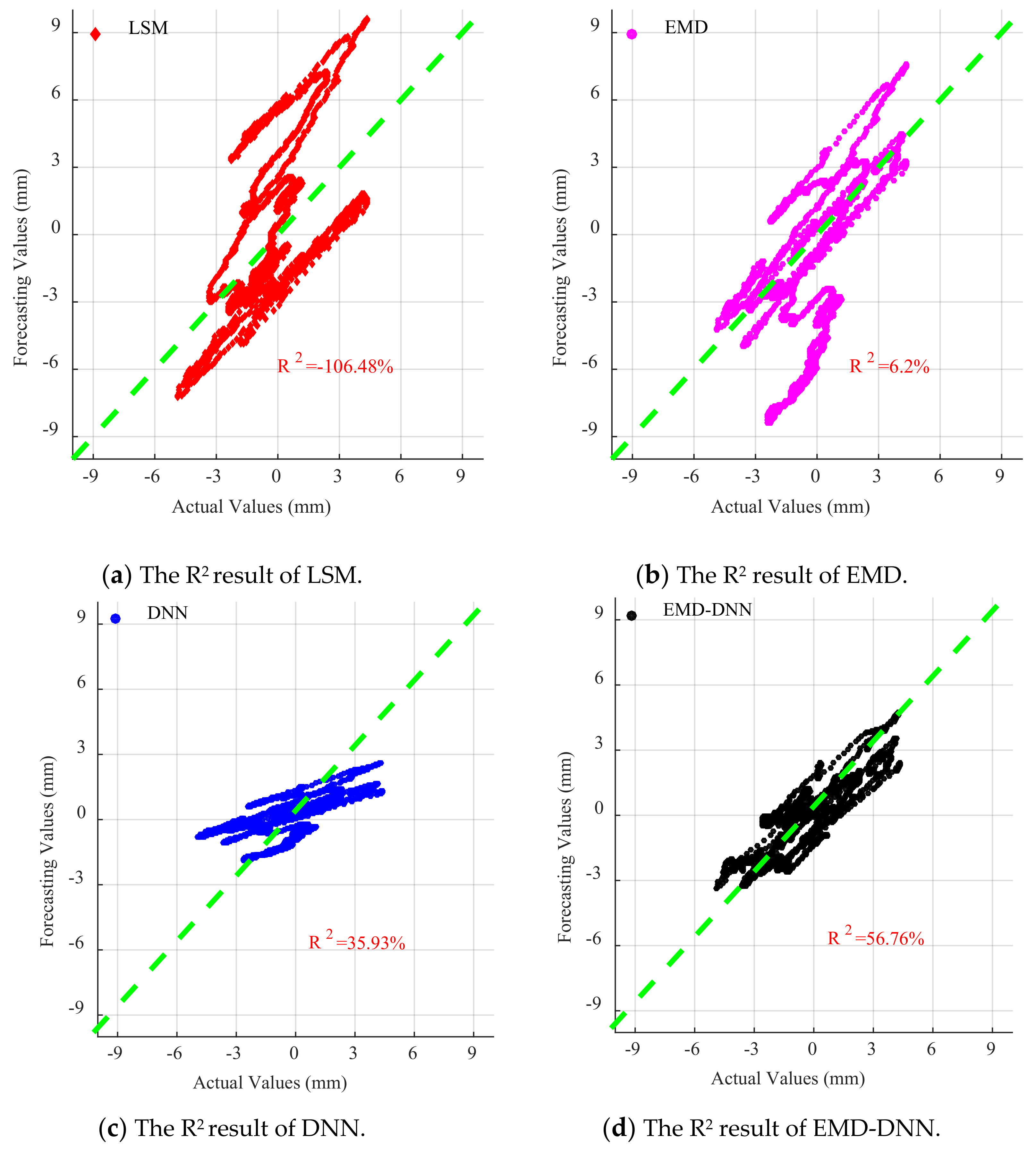
4.2. Results and Analyses
5. Concluding Remarks
- (1)
- The traditional least square method has a narrow scope of application and high discreteness. It is mostly used to solve the linear baseline drift caused by the inconsistency between the assumed initial value of velocity or displacement and the actual situation but cannot correct the acceleration error. The EMD applies to a wide range. The structural health monitoring data and shaking table data have specific baseline correction effects using the EMD. Both linear and nonlinear polynomial trends can be eliminated by removing RES items and reconstructing IMF by EMD.
- (2)
- The characteristics of drift displacement can be extracted directly by DNN, and the time history of drift displacement is taken as the sample set and input to the DNN model for training and prediction. From the evaluation index, it is shown that this method has a certain prediction effect on the real displacement response.
- (3)
- DNN can extract the features of multi-time-series IMF obtained by EMD decomposition, taking displacement time-history curves of different IMF components and drifting as the sample set, these are inputted into the DNN model for training and prediction; finally, improving real displacement response prediction accuracy. It can be obtained from various evaluation indexes that EMD–DNN has the highest accuracy compared with other methods.
- (4)
- In practical engineering applications, the EMD–DNN model can be trained only with the data of one displacement monitoring point to predict the actual displacement response of other positions. With this method, the sensor layout can be optimized in the shaking table test and actual structure monitoring, so as to reduce the number of displacement meter layouts and reduce the cost.
- (5)
- Since the EMD–DNN model needs to be obtained by real displacement training, we can conduct short-term displacement measurements for a monitoring point of the structure. After the EMD–DNN model is obtained by training, the real displacement response of each position of the structure can be predicted in the long term by the acceleration sensor, without the need of displacement sensor arrangement.
Author Contributions
Funding
Acknowledgments
Conflicts of Interest
References
- Chen, Z.; Tse, K.; Kwok, K.; Kareem, A.; Kim, B. Measurement of unsteady aerodynamic force on a galloping prism in a turbulent flow: A hybrid aeroelastic-pressure balance. J. Fluids Struct. 2021, 102, 103232. [Google Scholar] [CrossRef]
- Chen, Z.; Fu, X.; Xu, Y.; Li, C.Y.; Kim, B.; Tse, K. A perspective on the aerodynamics and aeroelasticity of tapering: Partial reattachment. J. Wind. Eng. Ind. Aerodyn. 2021, 212, 104590. [Google Scholar] [CrossRef]
- Zheng, W.; Dan, D.; Cheng, W.; Xia, Y. Real-time dynamic displacement monitoring with double integration of acceleration based on recursive least squares method. Measurement 2019, 141, 460–471. [Google Scholar] [CrossRef]
- Dai, Z.; Li, X.; Chen, S.; Zhao, S.; Xiong, Z. Baseline correction based on L1-Norm optimization and its verification by a computer vision method. Soil Dyn. Earthq. Eng. 2020, 131, 106047. [Google Scholar] [CrossRef]
- Iwan, W.D.; Moser, M.A.; Peng, C.Y. Some observations on strong-motion earthquake measurement using a digital accelerograph. Bull. Seismol. Soc. Am. 1985, 75, 1225–1246. [Google Scholar] [CrossRef]
- Chiu, H.-C. Stable baseline correction of digital strong-motion data. Bull. Seismol. Soc. Am. 1997, 87, 932–944. [Google Scholar] [CrossRef]
- Abrahamson, N.A.; Silva, W.J. Empirical Response Spectral Attenuation Relations for Shallow Crustal Earthquakes. Seismol. Res. Lett. 1997, 68, 94–127. [Google Scholar] [CrossRef] [Green Version]
- Athanasiou, A.; Oliveto, G.; Ponzo, F. Baseline Correction of Digital Accelerograms from Field Testing of a Seismically Isolated Building. Earthq. Spectra 2019, 34, 915–939. [Google Scholar] [CrossRef]
- Boore, D.M. Effect of baseline corrections on displacements and response spectra for several recordings of the 1999 Chi-Chi, Taiwan, earthquake. Bull. Seismol. Soc. Am. 2001, 91, 1199–1211. [Google Scholar] [CrossRef] [Green Version]
- Wang, R.; Schurr, B.; Milkereit, C.; Shao, Z.; Jin, M. An Improved Automatic Scheme for Empirical Baseline Correction of Digital Strong-Motion Records. Bull. Seismol. Soc. Am. 2011, 101, 2029–2044. [Google Scholar] [CrossRef]
- Wu, Y.-M.; Wu, C.-F. Approximate recovery of coseismic deformation from Taiwan strong-motion records. J. Seismol. 2007, 11, 159–170. [Google Scholar] [CrossRef]
- Boore, D.M.; Bommer, J.J. Processing of strong-motion accelerograms: Needs, options and consequences. Soil Dyn. Earthq. Eng. 2005, 25, 93–115. [Google Scholar] [CrossRef]
- Antoniou, S.; Pinho, R.; Bianchi, F. “SeismoSignal v5.1” A Computer Program for Signal Processing of Strong-Motion Data; Seismosoft Ltd.: Pavia, Italy, 2015. [Google Scholar]
- Pan, C.; Zhang, R.; Luo, H.; Shen, H. Target-based algorithm for baseline correction of inconsistent vibration signals. J. Vib. Control. 2017, 24, 2562–2575. [Google Scholar] [CrossRef]
- Lin, Y.; Zong, Z.; Tian, S.; Lin, J. A new baseline correction method for near-fault strong-motion records based on the target final displacement. Soil Dyn. Earthq. Eng. 2018, 114, 27–37. [Google Scholar] [CrossRef]
- Yang, G.; Dai, J.; Liu, X.; Chen, M.; Wu, X. Multiple Constrained Reweighted Penalized Least Squares for Spectral Baseline Correction. Appl. Spectrosc. 2020, 74, 1443–1451. [Google Scholar] [CrossRef] [PubMed]
- Huang, N.E.; Shen, Z.; Long, S.R.; Wu, M.C.; Shih, H.H.; Zheng, Q.; Yen, N.-C.; Tung, C.C.; Liu, H.H. The empirical mode decomposition and the Hilbert spectrum for nonlinear and non-stationary time series analysis. Proceedings of the Royal Society of London. Series A: Mathematical. Phys. Eng. Sci. 1998, 454, 903–995. [Google Scholar] [CrossRef]
- Xu, X.; Huo, X.; Qian, X.; Lu, X.; Yu, Q.; Ni, K.; Wang, X. Data-driven and coarse-to-fine baseline correction for signals of analytical instruments. Anal. Chim. Acta 2021, 1157, 338386. [Google Scholar] [CrossRef]
- Bao, Y.; Tang, Z.; Li, H.; Zhang, Y. Computer vision and deep learning–based data anomaly detection method for structural health monitoring. Struct. Health Monit. 2019, 18, 401–421. [Google Scholar] [CrossRef]
- Deng, Z.; Wang, B.; Xu, Y.; Xu, T.; Liu, C.; Zhu, Z. Multi-Scale Convolutional Neural Network With Time-Cognition for Multi-Step Short-Term Load Forecasting. IEEE Access. 2019, 7, 88058–88071. [Google Scholar] [CrossRef]
- Rumelhart, D.E.; Hinton, G.E.; Williams, R.J. Learning representations by back-propagating errors. Nature 1986, 323, 533–536. [Google Scholar] [CrossRef]
- Qian, N. On the momentum term in gradient descent learning algorithms. Neural Netw. 1999, 12, 145–151. [Google Scholar] [CrossRef]
- Duchi, J.; Hazan, E.; Singer, Y. Adaptive Subgradient Methods for Online Learning and Stochastic Optimization. J. Mach. Learn. Res. 2011, 12, 2121–2159. [Google Scholar]
- Yi, D.; Ahn, J.; Ji, S. An Effective Optimization Method for Machine Learning Based on ADAM. Appl. Sci. 2020, 10, 1073. [Google Scholar] [CrossRef] [Green Version]
- Ye, Y.; Wang, Z.; Zhang, X. An optimal pointwise weighted ensemble of surrogates based on minimization of local mean square error. Struct. Multidiscip. Optim. 2020, 62, 529–542. [Google Scholar] [CrossRef]
- Ćalasan, M.; Aleem, S.H.A.; Zobaa, A.F. On the root mean square error (RMSE) calculation for parameter estimation of photovoltaic models: A novel exact analytical solution based on Lambert W function. Energy Convers. Manag. 2020, 210, 112716. [Google Scholar] [CrossRef]
- Yang, X.; Park, G.-K.; Hu, Y. Least absolute deviations estimation for uncertain autoregressive model. Soft Comput. 2020, 24, 18211–18217. [Google Scholar] [CrossRef]
- Kasuya, E. On the use of r and r squared in correlation and regression. Ecol. Res. 2018, 34, 235–236. [Google Scholar] [CrossRef]


| Method | Time of Establishment | Advantages | Disadvantages |
|---|---|---|---|
| Iwan | 1985 | Simple and convenient | Parameter selection is fixed, only applicable to specific accelerometers |
| V0 | 2001 | The selection of parameters has great physical meaning | Parameter calculation relies on subjective experience, which makes it easier to introduce errors |
| Wu and Wu | 2007 | The result of bilinear correction has high accuracy | Parameter selection depends on the preset threshold |
| Automatic iteration | 2011 | As far as possible to ensure the accuracy of parameter selection, reduce the subjective error | The calculation process is complicated, and the efficiency is relatively low |
| Number | Sensor Type |
|---|---|
| A | ENDEVCO acceleration sensor |
| B | Unimeasure pull-wire displacement meter |
Publisher’s Note: MDPI stays neutral with regard to jurisdictional claims in published maps and institutional affiliations. |
© 2021 by the authors. Licensee MDPI, Basel, Switzerland. This article is an open access article distributed under the terms and conditions of the Creative Commons Attribution (CC BY) license (https://creativecommons.org/licenses/by/4.0/).
Share and Cite
Chen, Z.; Fu, J.; Peng, Y.; Chen, T.; Zhang, L.; Yuan, C. Baseline Correction of Acceleration Data Based on a Hybrid EMD–DNN Method. Sensors 2021, 21, 6283. https://doi.org/10.3390/s21186283
Chen Z, Fu J, Peng Y, Chen T, Zhang L, Yuan C. Baseline Correction of Acceleration Data Based on a Hybrid EMD–DNN Method. Sensors. 2021; 21(18):6283. https://doi.org/10.3390/s21186283
Chicago/Turabian StyleChen, Zengshun, Jun Fu, Yanjian Peng, Tuanhai Chen, LiKai Zhang, and Chenfeng Yuan. 2021. "Baseline Correction of Acceleration Data Based on a Hybrid EMD–DNN Method" Sensors 21, no. 18: 6283. https://doi.org/10.3390/s21186283
APA StyleChen, Z., Fu, J., Peng, Y., Chen, T., Zhang, L., & Yuan, C. (2021). Baseline Correction of Acceleration Data Based on a Hybrid EMD–DNN Method. Sensors, 21(18), 6283. https://doi.org/10.3390/s21186283