
Reliability of IMU-Based Gait Assessment in Clinical Stroke Rehabilitation

 ,
,  ,
,
Abstract
:1. Introduction
2. Materials and Methods
2.1. Participants
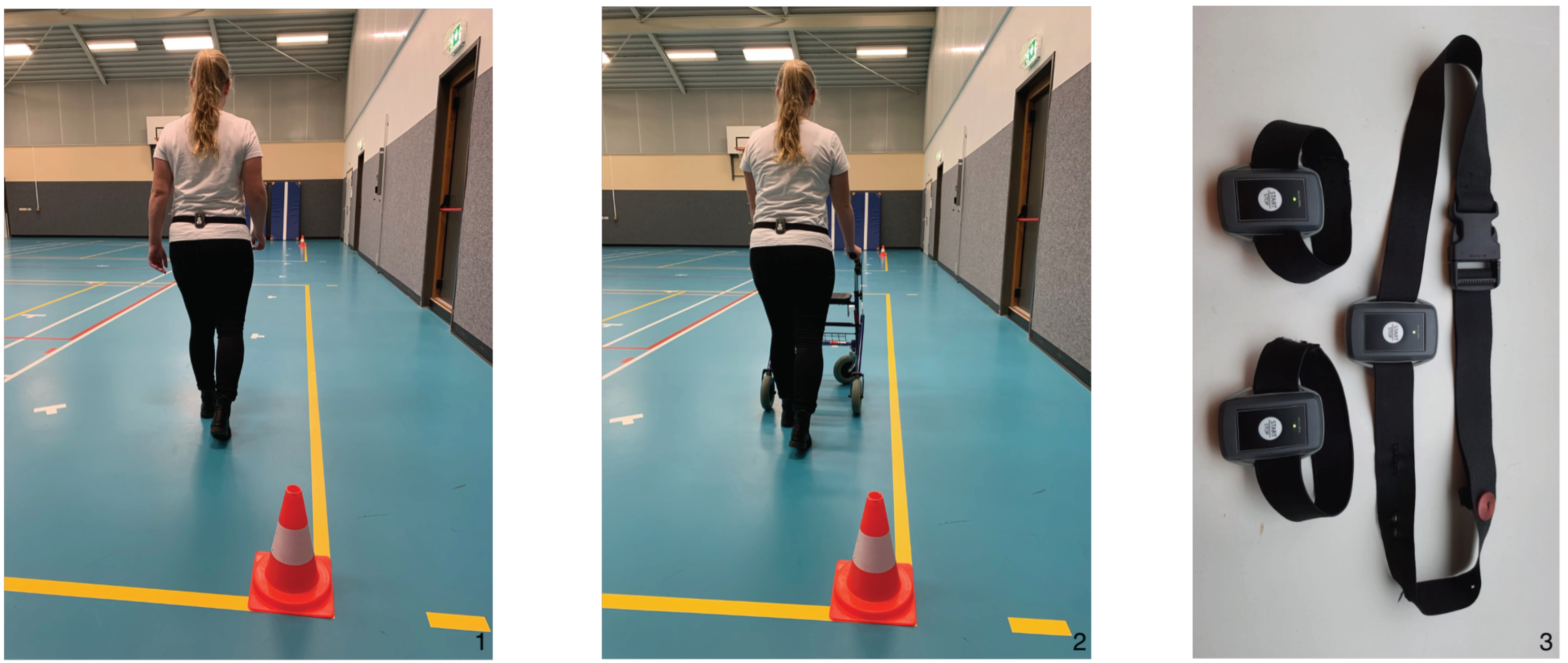
2.2. Protocol
2.3. Equipment
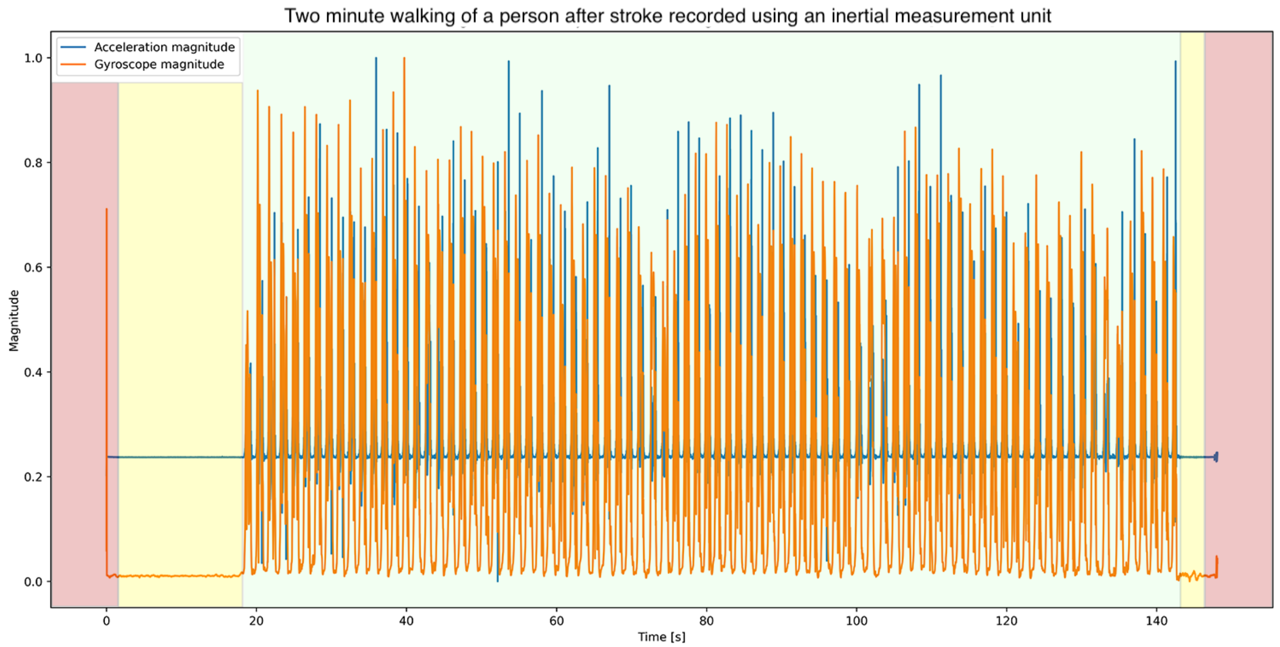
2.4. Data Processing
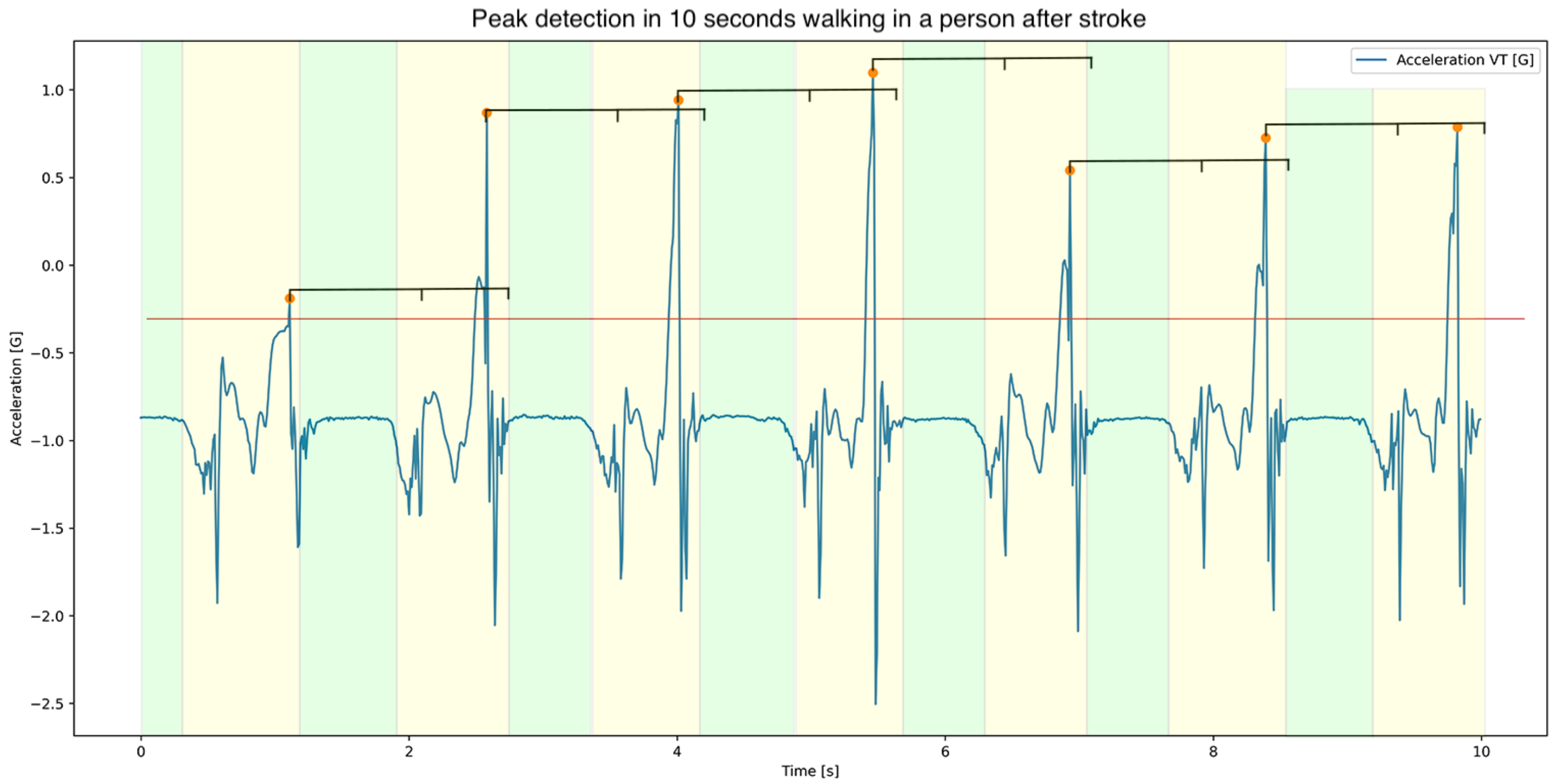
2.5. Stride Detection
2.6. Calculations
2.7. Statistics
3. Results
3.1. Descriptives
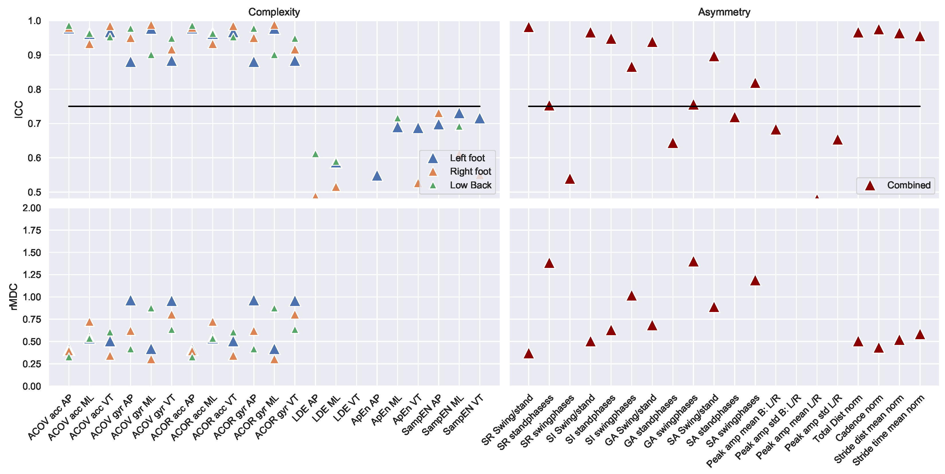
3.2. Reliability
3.3. Clinical Monitoring
4. Discussion
5. Conclusions
Author Contributions
Funding
Institutional Review Board Statement
Informed Consent Statement
Data Availability Statement
Acknowledgments
Conflicts of Interest
Abbreviations
| IMU | Inertial measurement Unit |
| L5/S1 | Lumbosacral joint |
| m/s2 | Metres per second squared |
| /s | Degrees per second |
| VT | Vertical |
| ML | Medio-lateral |
| AP | Anterior–posterior |
| ICC | Intraclass correlation coefficient |
| MDC | Minimal detectable change |
| SEM | Standard error of measurement |
| rMDC | Relative minimal detectable change |
Appendix A

| Reliability | Test | Retest | |||||
|---|---|---|---|---|---|---|---|
| ICC (−CI, CI) | MDC (SEM) | rMDC | Mean (STD) | Mean (STD) | |||
| Left Foot | Spatio-Temporal | 1. Stride time mean L | 0.965 (0.92,0.98) | 0.355 (0.128) | 0.52 | 1.767 (0.72) | 1.701 (0.64) |
| 2. Stride time std L | 0.823 (0.65,0.92) | 0.144 (0.052) | 1.17 | 0.168 (0.121) | 0.162 (0.126) | ||
| 3. Stride time norm L | 0.798 (0.6,0.9) | 0.087 (0.031) | 1.26 | 0.092 (0.06) | 0.097 (0.078) | ||
| 4. Stride dist mean L | 0.963 (0.92,0.98) | 0.142 (0.051) | 0.53 | 0.71 (0.258) | 0.706 (0.271) | ||
| 5. Stride dist std L | 0.835 (0.67,0.92) | 0.038 (0.014) | 1.12 | 0.087 (0.034) | 0.089 (0.034) | ||
| 6. KMPH L | 0.97 (0.94,0.99) | 0.482 (0.174) | 0.48 | 1.659 (0.991) | 1.715 (1.016) | ||
| 7. Cadence L | 0.969 (0.93,0.99) | 5.829 (2.103) | 0.49 | 38.556 (11.967) | 39.37 (11.864) | ||
| 8. Stride vel mean L | 0.952 (0.9,0.98) | 0.389 (0.14) | 0.61 | 1.367 (0.638) | 1.358 (0.637) | ||
| 9. Stride vel std L | 0.779 (0.56,0.89) | 0.312 (0.112) | 1.36 | 0.286 (0.168) | 0.347 (0.291) | ||
| 10. Range acc AP L | 0.862 (0.72,0.93) | 17.733 (6.398) | 1.03 | 49.86 (16.244) | 50.769 (18.121) | ||
| 11. RMS acc AP L | 0.907 (0.81,0.96) | 2.323 (0.838) | 0.85 | 5.014 (2.716) | 5.201 (2.781) | ||
| 12. Range acc ML L | 0.672 (0.4,0.84) | 45.144 (12.288) | 44.367 (12.724) | ||||
| 13. RMS acc ML L | 0.761 (0.54,0.88) | 2.66 (0.96) | 1.36 | 4.024 (1.884) | 4.074 (2.041) | ||
| 14. Range acc VT L | 0.758 (0.53,0.88) | 22.779 (8.218) | 1.37 | 48.206 (16.406) | 47.376 (16.964) | ||
| 15. RMS acc VT L | 0.96 (0.91,0.98) | 1.241 (0.448) | 0.56 | 3.652 (2.101) | 3.769 (2.342) | ||
| 16. Range gyr AP L | 0.882 (0.76,0.94) | 2.98 (1.075) | 0.95 | 7.724 (3.058) | 7.982 (3.188) | ||
| 17. RMS gyr AP L | 0.748 (0.52,0.88) | 1.15 (0.637) | 1.176 (0.658) | ||||
| 18. Range gyr ML L | 0.918 (0.83,0.96) | 3.114 (1.123) | 0.79 | 9.338 (3.827) | 9.423 (4.031) | ||
| 19. RMS gyr ML L | 0.923 (0.84,0.96) | 0.688 (0.248) | 0.77 | 1.558 (0.861) | 1.605 (0.929) | ||
| 20. Range gyr VT L | 0.928 (0.85,0.97) | 1.597 (0.576) | 0.74 | 6.666 (2.183) | 6.898 (2.117) | ||
| 21. RMS gyr VT L | 0.94 (0.87,0.97) | 0.198 (0.071) | 0.68 | 0.774 (0.28) | 0.81 (0.3) | ||
| Frequency | 22. Dominant peak freq L | 0.638 (0.34,0.82) | 0.061 (0.035) | 0.061 (0.033) | |||
| 23. Dominant peak width L | −0.001 (−0.36,0.36) | −3.105 (13.092) | 0.575 (0.096) | ||||
| 24. Dominant peak slope L | 0.599 (0.29,0.8) | 0.001 (0.001) | 0.001 (0.001) | ||||
| 25. Dominant peak density L | 0.655 (0.37,0.83) | 0.189 (0.104) | 0.183 (0.093) | ||||
| Complexity | 26. ACOV acc AP L | 0.979 (0.94,0.99) | 0.074 (0.027) | 0.41 | 0.123 (0.174) | 0.141 (0.19) | |
| 27. ACOV acc ML L | 0.962 (0.92,0.98) | 0.026 (0.009) | 0.54 | 0.031 (0.045) | 0.035 (0.05) | ||
| 28. ACOV acc VT L | 0.967 (0.92,0.99) | 0.07 (0.025) | 0.5 | 0.081 (0.13) | 0.096 (0.147) | ||
| 29. ACOV gyr AP L | 0.881 (0.74,0.95) | 0.261 (0.094) | 0.97 | 0.219 (0.245) | 0.271 (0.297) | ||
| 30. ACOV gyr ML L | 0.977 (0.93,0.99) | 1.588 (0.573) | 0.42 | 3.093 (3.592) | 3.534 (3.978) | ||
| 31. ACOV gyr VT L | 0.884 (0.76,0.95) | 0.612 (0.221) | 0.96 | 0.478 (0.743) | 0.435 (0.533) | ||
| 32. ACOR acc AP L | 0.979 (0.94,0.99) | 0.074 (0.027) | 0.41 | 0.123 (0.174) | 0.141 (0.19) | ||
| 33. ACOR acc ML L | 0.962 (0.92,0.98) | 0.026 (0.009) | 0.54 | 0.031 (0.045) | 0.035 (0.05) | ||
| 34. ACOR acc VT L | 0.967 (0.92,0.99) | 0.07 (0.025) | 0.5 | 0.081 (0.13) | 0.096 (0.147) | ||
| 35. ACOR gyr AP L | 0.881 (0.74,0.95) | 0.261 (0.094) | 0.97 | 0.219 (0.245) | 0.271 (0.297) | ||
| 36. ACOR gyr ML L | 0.977 (0.93,0.99) | 1.588 (0.573) | 0.42 | 3.093 (3.592) | 3.534 (3.978) | ||
| 37. ACOR gyr VT L | 0.884 (0.76,0.95) | 0.612 (0.221) | 0.96 | 0.478 (0.743) | 0.435 (0.533) | ||
| 38. LDE AP L | 0.322 (−0.06,0.62) | 0.009 (0.002) | 0.009 (0.002) | ||||
| 39. LDE ML L | 0.587 (0.27,0.79) | 0.007 (0.001) | 0.007 (0.002) | ||||
| 40. LDE VT L | 0.208 (−0.19,0.54) | 0.009 (0.002) | 0.009 (0.002) | ||||
| 41. ApproxE AP L | 0.549 (0.22,0.77) | 0.388 (0.118) | 0.377 (0.134) | ||||
| 42. ApproxE ML L | 0.69 (0.43,0.85) | 0.514 (0.151) | 0.495 (0.167) | ||||
| 43. ApproxE VT L | 0.688 (0.43,0.84) | 0.369 (0.11) | 0.352 (0.119) | ||||
| 44. SampE AP L | 0.698 (0.44,0.85) | 0.08 (0.037) | 0.077 (0.039) | ||||
| 45. SampE ML L | 0.731 (0.49,0.87) | 0.15 (0.068) | 0.145 (0.083) | ||||
| 46. SampE VT L | 0.716 (0.47,0.86) | 0.091 (0.041) | 0.087 (0.048) | ||||
| Right Foot | Spatio-Temporal | 47. Stride time mean R | 0.938 (0.86,0.97) | 0.469 (0.169) | 0.69 | 1.775 (0.73) | 1.69 (0.623) |
| 48. Stride time std R | 0.636 (0.35,0.82) | 0.184 (0.18) | 0.164 (0.108) | ||||
| 49. Stride time norm R | 0.686 (0.42,0.84) | 0.099 (0.061) | 0.099 (0.062) | ||||
| 50. Stride dist mean R | 0.956 (0.91,0.98) | 0.144 (0.052) | 0.58 | 0.671 (0.233) | 0.676 (0.262) | ||
| 51. Stride dist std R | 0.781 (0.57,0.89) | 0.073 (0.026) | 1.3 | 0.121 (0.061) | 0.119 (0.051) | ||
| 52. KMPH R | 0.963 (0.92,0.98) | 0.494 (0.178) | 0.53 | 1.56 (0.881) | 1.642 (0.974) | ||
| 53. Cadence R | 0.977 (0.95,0.99) | 4.992 (1.801) | 0.42 | 38.407 (11.849) | 39.37 (11.833) | ||
| 54. Stride vel mean R | 0.967 (0.93,0.98) | 0.289 (0.104) | 0.51 | 1.267 (0.555) | 1.28 (0.588) | ||
| 55. Stride vel std R | 0.939 (0.87,0.97) | 0.17 (0.061) | 0.69 | 0.327 (0.23) | 0.347 (0.264) | ||
| 56. Range acc AP R | 0.9 (0.8,0.95) | 17.789 (6.418) | 0.88 | 53.188 (18.792) | 54.961 (21.676) | ||
| 57. RMS acc AP R | 0.905 (0.8,0.96) | 2.14 (0.772) | 0.85 | 5.061 (2.446) | 5.067 (2.562) | ||
| 58. Range acc MR R | 0.8 (0.61,0.9) | 20.705 (7.47) | 1.24 | 47.718 (17.953) | 49.285 (15.333) | ||
| 59. RMS acc MR R | 0.826 (0.64,0.92) | 2.351 (0.848) | 1.17 | 3.692 (1.838) | 4.16 (2.19) | ||
| 60. Range acc VT R | 0.936 (0.87,0.97) | 18.685 (6.741) | 0.7 | 51.447 (25.79) | 51.871 (27.648) | ||
| 61. RMS acc VT R | 0.971 (0.94,0.99) | 1.131 (0.408) | 0.47 | 3.78 (2.313) | 3.952 (2.487) | ||
| 62. Range gyr AP R | 0.825 (0.65,0.92) | 3.707 (1.337) | 1.16 | 7.847 (3.024) | 8.398 (3.341) | ||
| 63. RMS gyr AP R | 0.797 (0.61,0.9) | 0.812 (0.293) | 1.26 | 1.093 (0.593) | 1.21 (0.698) | ||
| 64. Range gyr MR R | 0.907 (0.81,0.96) | 3.318 (1.197) | 0.85 | 9.94 (3.742) | 9.852 (4.097) | ||
| 65. RMS gyr MR R | 0.863 (0.72,0.94) | 0.826 (0.298) | 1.03 | 1.695 (0.774) | 1.648 (0.834) | ||
| 66. Range gyr VT R | 0.931 (0.86,0.97) | 1.52 (0.548) | 0.73 | 6.285 (2.079) | 6.46 (2.079) | ||
| Frequency | 68. Dominant peak freq R | 0.828 (0.65,0.92) | 0.053 (0.019) | 1.16 | 0.074 (0.048) | 0.065 (0.044) | |
| 69. Dominant peak width R | −0.006 (−0.32,0.34) | 0.609 (0.004) | 0.564 (0.108) | ||||
| 70. Dominant peak slope R | 0.823 (0.65,0.92) | 0.001 (0.0) | 1.17 | 0.001 (0.001) | 0.001 (0.001) | ||
| 71. Dominant peak density R | 0.889 (0.77,0.95) | 0.117 (0.042) | 0.92 | 0.204 (0.126) | 0.193 (0.127) | ||
| Complexity | 72. ACOV acc AP R | 0.98 (0.95,0.99) | 0.077 (0.028) | 0.39 | 0.126 (0.187) | 0.145 (0.208) | |
| 73. ACOV acc MR R | 0.933 (0.85,0.97) | 0.035 (0.013) | 0.72 | 0.027 (0.045) | 0.034 (0.051) | ||
| 74. ACOV acc VT R | 0.985 (0.97,0.99) | 0.047 (0.017) | 0.34 | 0.083 (0.133) | 0.09 (0.143) | ||
| 75. ACOV gyr AP R | 0.95 (0.89,0.98) | 0.234 (0.084) | 0.62 | 0.235 (0.379) | 0.279 (0.375) | ||
| 76. ACOV gyr MR R | 0.988 (0.97,0.99) | 1.102 (0.398) | 0.3 | 3.081 (3.572) | 3.318 (3.703) | ||
| 77. ACOV gyr VT R | 0.916 (0.82,0.96) | 0.554 (0.2) | 0.8 | 0.415 (0.663) | 0.51 (0.715) | ||
| 78. ACOR acc AP R | 0.98 (0.95,0.99) | 0.077 (0.028) | 0.39 | 0.126 (0.187) | 0.145 (0.208) | ||
| 79. ACOR acc MR R | 0.933 (0.85,0.97) | 0.035 (0.013) | 0.72 | 0.027 (0.045) | 0.034 (0.051) | ||
| 80. ACOR acc VT R | 0.985 (0.97,0.99) | 0.047 (0.017) | 0.34 | 0.083 (0.133) | 0.09 (0.143) | ||
| 81. ACOR gyr AP R | 0.95 (0.89,0.98) | 0.234 (0.084) | 0.62 | 0.235 (0.379) | 0.279 (0.375) | ||
| 82. ACOR gyr MR R | 0.988 (0.97,0.99) | 1.102 (0.398) | 0.3 | 3.081 (3.572) | 3.318 (3.703) | ||
| 83. ACOR gyr VT R | 0.916 (0.82,0.96) | 0.554 (0.2) | 0.8 | 0.415 (0.663) | 0.51 (0.715) | ||
| 84. LDE AP R | 0.487 (0.13,0.73) | 0.01 (0.002) | 0.01 (0.002) | ||||
| 85. LDE MR R | 0.516 (0.19,0.74) | 0.007 (0.001) | 0.007 (0.002) | ||||
| 86. LDE VT R | 0.056 (−0.34,0.43) | 0.009 (0.002) | 0.009 (0.001) | ||||
| 87. ApproxE AP R | 0.441 (0.07,0.7) | 0.388 (0.123) | 0.389 (0.136) | ||||
| 88. ApproxE MR R | 0.344 (−0.04,0.64) | 0.53 (0.14) | 0.514 (0.159) | ||||
| 89. ApproxE VT R | 0.527 (0.19,0.75) | 0.366 (0.103) | 0.38 (0.114) | ||||
| 90. SampE AP R | 0.731 (0.49,0.87) | 0.08 (0.042) | 0.084 (0.043) | ||||
| 91. SampE MR R | 0.611 (0.3,0.8) | 0.156 (0.066) | 0.154 (0.062) | ||||
| 92. SampE VT R | 0.55 (0.22,0.77) | 0.095 (0.046) | 0.101 (0.044) | ||||
| Low Back | Spatio-Temporal | 93. Step time mean B | 0.955 (0.9,0.98) | 0.197 (0.071) | 0.59 | 0.877 (0.354) | 0.846 (0.317) |
| 94. Step time std B | 0.698 (0.44,0.85) | 0.3 (0.172) | 0.257 (0.135) | ||||
| 95. Step time norm B | 0.686 (0.42,0.84) | 0.395 (0.157) | 0.352 (0.161) | ||||
| 96. Range acc AP B | 0.922 (0.84,0.96) | 0.191 (0.069) | 0.78 | 0.572 (0.245) | 0.579 (0.249) | ||
| 97. Rms acc AP B | 0.949 (0.88,0.98) | 0.022 (0.008) | 0.63 | 0.093 (0.036) | 0.097 (0.035) | ||
| 98. Range acc ML B | 0.845 (0.69,0.93) | 0.374 (0.135) | 1.11 | 0.657 (0.283) | 0.709 (0.392) | ||
| 99. Rms acc ML B | 0.511 (0.17,0.74) | 0.114 (0.026) | 0.117 (0.041) | ||||
| 100. Range acc VT B | 0.945 (0.88,0.97) | 0.253 (0.091) | 0.65 | 0.755 (0.362) | 0.763 (0.416) | ||
| 101. Rms acc VT B | 0.804 (0.61,0.91) | 0.023 (0.008) | 1.24 | 0.998 (0.019) | 1.002 (0.018) | ||
| 102. Range gyr AP B | 0.972 (0.94,0.99) | 0.313 (0.113) | 0.46 | 1.199 (0.646) | 1.228 (0.707) | ||
| 103. Rms gyr AP B | 0.972 (0.94,0.99) | 0.049 (0.018) | 0.46 | 0.184 (0.1) | 0.193 (0.111) | ||
| 104. Range gyr ML B | 0.76 (0.54,0.88) | 0.907 (0.327) | 1.38 | 1.527 (0.762) | 1.434 (0.556) | ||
| 105. Rms gyr ML B | 0.849 (0.7,0.93) | 0.092 (0.033) | 1.08 | 0.227 (0.086) | 0.224 (0.085) | ||
| 106. Range gyr VT B | 0.93 (0.85,0.97) | 0.629 (0.227) | 0.74 | 1.861 (0.782) | 1.929 (0.926) | ||
| 107. Rms gyr VT B | 0.962 (0.92,0.98) | 0.087 (0.031) | 0.54 | 0.342 (0.151) | 0.356 (0.168) | ||
| Frequency | 108. Dominant peak freq AP B | 0.713 (0.46,0.86) | 0.123 (0.055) | 0.117 (0.054) | |||
| 109. Dominant peak width AP B | −0.011 (−0.35,0.35) | 0.609 (0.005) | 0.576 (0.096) | ||||
| 110. Dominant peak slope AP B | 0.735 (0.5,0.87) | 0.002 (0.001) | 0.002 (0.001) | ||||
| 111. Dominant peak density AP B | 0.715 (0.46,0.86) | 0.356 (0.152) | 0.356 (0.173) | ||||
| 112. HR AP B | 0.847 (0.69,0.93) | 1.162 (0.419) | 1.09 | 1.418 (1.034) | 1.497 (1.105) | ||
| 113. IH AP B | 0.456 (0.09,0.71) | 0.586 (0.089) | 0.588 (0.125) | ||||
| 114. Dominant peak freq ML B | 0.657 (0.26,0.85) | 0.125 (0.052) | 0.101 (0.043) | ||||
| 115. Dominant peak width ML B | −0.0 (−0.37,0.37) | 0.608 (0.008) | −1.276 (9.436) | ||||
| 116. Dominant peak slope ML B | 0.657 (0.23,0.85) | 0.002 (0.001) | 0.002 (0.001) | ||||
| 117. Dominant peak density ML B | 0.771 (0.56,0.89) | 0.192 (0.069) | 1.34 | 0.344 (0.139) | 0.311 (0.148) | ||
| 118. HR ML B | 0.86 (0.66,0.94) | 0.63 (0.227) | 1.06 | 1.824 (0.678) | 1.662 (0.515) | ||
| 119. IH ML B | 0.809 (0.61,0.91) | 0.16 (0.058) | 1.22 | 0.474 (0.136) | 0.442 (0.126) | ||
| 120. Dominant peak freq VT B | 0.584 (0.27,0.79) | 0.104 (0.053) | 0.097 (0.052) | ||||
| 121. Dominant peak width VT B | 0.004 (−0.33,0.36) | 0.609 (0.004) | 0.575 (0.096) | ||||
| 122. Dominant peak slope VT B | 0.614 (0.31,0.8) | 0.002 (0.001) | 0.002 (0.001) | ||||
| 123. Dominant peak density VT B | 0.616 (0.31,0.81) | 0.306 (0.156) | 0.301 (0.167) | ||||
| 124. HR VT B | 0.931 (0.86,0.97) | 0.732 (0.264) | 0.73 | 1.768 (0.999) | 1.794 (1.018) | ||
| Complexity | 126. ACOV acc AP B | 0.986 (0.97,0.99) | 0.004 (0.002) | 0.33 | 0.007 (0.013) | 0.008 (0.014) | |
| 127. ACOV acc ML B | 0.963 (0.91,0.98) | 0.001 (0.001) | 0.53 | 0.003 (0.003) | 0.004 (0.003) | ||
| 128. ACOV acc VT B | 0.952 (0.9,0.98) | 0.004 (0.001) | 0.61 | 0.007 (0.006) | 0.007 (0.007) | ||
| 129. ACOV gyr AP B | 0.978 (0.95,0.99) | 0.043 (0.016) | 0.42 | 0.091 (0.098) | 0.099 (0.109) | ||
| 130. ACOV gyr ML B | 0.901 (0.8,0.95) | 0.026 (0.009) | 0.87 | 0.034 (0.028) | 0.037 (0.031) | ||
| 131. ACOV gyr VT B | 0.948 (0.87,0.98) | 0.03 (0.011) | 0.63 | 0.031 (0.043) | 0.038 (0.051) | ||
| 132. ACOR acc AP B | 0.986 (0.97,0.99) | 0.004 (0.002) | 0.33 | 0.007 (0.013) | 0.008 (0.014) | ||
| 133. ACOR acc ML B | 0.963 (0.91,0.98) | 0.001 (0.001) | 0.53 | 0.003 (0.003) | 0.004 (0.003) | ||
| 134. ACOR acc VT B | 0.952 (0.9,0.98) | 0.004 (0.001) | 0.61 | 0.007 (0.006) | 0.007 (0.007) | ||
| 135. ACOR gyr AP B | 0.978 (0.95,0.99) | 0.043 (0.016) | 0.42 | 0.091 (0.098) | 0.099 (0.109) | ||
| 136. ACOR gyr ML B | 0.901 (0.8,0.95) | 0.026 (0.009) | 0.87 | 0.034 (0.028) | 0.037 (0.031) | ||
| 137. ACOR gyr VT B | 0.948 (0.87,0.98) | 0.03 (0.011) | 0.63 | 0.031 (0.043) | 0.038 (0.051) | ||
| 138. LDE AP B | 0.612 (0.3,0.8) | 0.014 (0.001) | 0.014 (0.001) | ||||
| 139. LDE ML B | 0.589 (0.28,0.79) | 0.014 (0.001) | 0.014 (0.001) | ||||
| 140. LDE VT B | 0.205 (−0.2,0.54) | 0.014 (0.001) | 0.014 (0.001) | ||||
| 141. ApproxE AP B | 0.124 (−0.24,0.47) | 0.61 (0.146) | 0.554 (0.148) | ||||
| 142. ApproxE ML B | 0.716 (0.46,0.86) | 0.606 (0.137) | 0.563 (0.16) | ||||
| 143. ApproxE VT B | 0.373 (0.02,0.65) | 0.51 (0.155) | 0.458 (0.156) | ||||
| 144. SampE AP B | 0.118 (−0.25,0.46) | 0.474 (0.179) | 0.41 (0.165) | ||||
| 145. SampE ML B | 0.692 (0.41,0.85) | 0.488 (0.158) | 0.431 (0.181) | ||||
| 146. SampE VT B | 0.208 (−0.16,0.53) | 0.363 (0.157) | 0.308 (0.131) | ||||
| Asymmetry | Spatio-Temporal | 147. SR Swing/stand | 0.982 (0.96,0.99) | 1.217 (0.439) | 0.37 | 2.234 (3.429) | 2.173 (3.116) |
| 148. SR standphasess | 0.753 (0.53,0.88) | 0.278 (0.1) | 1.39 | 0.902 (0.224) | 0.904 (0.178) | ||
| 149. SR swingphases | 0.54 (0.21,0.76) | 1.278 (0.725) | 1.166 (0.291) | ||||
| 150. SI Swing/stand | 0.967 (0.93,0.98) | 92.302 (33.3) | 0.5 | 169.709 (179.456) | 164.206 (186.235) | ||
| 151. SI standphases | 0.948 (0.89,0.98) | 0.435 (0.157) | 0.63 | 1.351 (0.677) | 1.395 (0.703) | ||
| 152. SI swingphases | 0.866 (0.73,0.94) | 0.422 (0.152) | 1.02 | 1.402 (0.454) | 1.405 (0.373) | ||
| 153. GA Swing/stand | 0.939 (0.87,0.97) | 51.278 (18.499) | 0.69 | 35.903 (73.448) | 34.233 (75.94) | ||
| 154. GA standphases | 0.644 (0.36,0.82) | −14.808 (33.798) | −12.298 (21.988) | ||||
| 155. GA swingphases | 0.756 (0.54,0.88) | 40.972 (14.781) | 1.4 | 16.052 (35.568) | 12.617 (22.82) | ||
| 156. SA Swing/stand | 0.897 (0.79,0.95) | 0.002 (0.001) | 0.89 | 0.49 (0.003) | 0.49 (0.003) | ||
| 157. SA standphases | 0.719 (0.47,0.86) | 0.492 (0.002) | 0.492 (0.001) | ||||
| 158. SA swingphases | 0.819 (0.64,0.91) | 0.002 (0.001) | 1.19 | 0.49 (0.002) | 0.491 (0.001) | ||
| 159. Peak amp mean B: L/R | 0.684 (0.42,0.84) | 0.141 (0.084) | 0.13 (0.068) | ||||
| 160. Peak amp std B: L/R | 0.244 (−0.14,0.57) | 0.989 (0.096) | 1.012 (0.108) | ||||
| 161. Peak amp mean L/R | 0.478 (0.14,0.72) | 0.536 (1.786) | −0.194 (2.005) | ||||
| 162. Peak amp std L/R | 0.654 (0.38,0.83) | 0.577 (0.249) | 0.653 (0.305) | ||||
| 163. Total Dist norm | 0.967 (0.93,0.98) | 0.093 (0.033) | 0.51 | 0.311 (0.178) | 0.323 (0.189) | ||
| 164. Cadence norm | 0.976 (0.95,0.99) | 0.031 (0.011) | 0.43 | 0.224 (0.071) | 0.229 (0.07) | ||
| 165. Stride dist mean norm | 0.964 (0.92,0.98) | 0.133 (0.048) | 0.52 | 0.69 (0.244) | 0.691 (0.266) | ||
| 166. Stride time mean norm | 0.956 (0.9,0.98) | 0.047 (0.017) | 0.59 | 0.209 (0.084) | 0.202 (0.075) | ||
Appendix B. Testing of the Stride Detection Algorithm
Appendix B.1. Protocol

Appendix B.2. Outcomes
| Measurement | Mean (SD) (min, max) | Pearson’s r | Root Mean Square Error | Absolute Average Difference | |
|---|---|---|---|---|---|
| Strides left foot | GS | 49.3 (15.5) (27, 88) | r(28) = 0.97, p < 0.01 | 3.90 | 1.96 |
| SDA | 48.4 (16.1) (24, 88) | ||||
| Strides right foot | GS | 49.3 (15.5) (27, 88) | r(28) = 0.98, p < 0.01 | 3.36 | 1.60 |
| SDA | 47.8 (16.2) (23, 88) | ||||
| Steps low back | GS | 98.5 (31.0) (53, 176) | r(28) = 0.98, p < 0.01 | 6.51 | 2.46 |
| SDA | 97.2 (32.7) (47, 178) | ||||
| Distance left foot | GS | 29.9 (22,6) (7.6, 105.6) | r(28) = 0.97, p < 0.01 | 5.93 | 4.11 |
| SDA | 30.9 (21.0) (8.1, 97.8) | ||||
| Distance right foot | GS | 29.9 (22.6) (7.6, 105.6) | r(28) = 0.97, p < 0.01 | 5.69 | 3.90 |
| SDA | 32.3 (22.1 (8.1, 109.6) |
Appendix C. Formulas
| Abbreviation | Description | Formulas: Spatio-Temporal and Frequency |
|---|---|---|
| Spatio-Temporal Features | ||
| Range | Range (m/s2, rad/s) (Features: 10, 12, 14, 16, 18, 20, 56, 58, 60, 62, 64, 66, 96, 98, 100, 102, 104, 106) | |
| STD | Standard deviation (m/s2, rad/s) (Features: 2, 5, 9, 48, 51, 55, 94, 160, 162) | |
| RMS | Root mean square (m/s2, rad/s) (Features: 11, 13, 15, 17, 19, 21, 57, 59, 63, 65, 67, 97, 99, 101, 103, 105, 107) | |
| Velocity | Velocity per stride [41] (m/s) (Features: 8, 9, 54, 55) | |
| Distance | Distance per stride (m) (Features: 4, 5, 50, 51) | |
| KMPH | Kilometres per hour (km/h) (Features: 6, 52) | |
| Cadence | Number of steps per minute (Features: 7, 53) | |
| Frequency features | ||
| FFT | Fast Fourier Transform of acceleration [39] | |
| Dominant peak freq | Dominant frequency in the signal indicating step or stride frequency (Hz) (Features: 22, 68, 108) | |
| Dominant peak width | Width of the peak of the dominant frequency (HZ) (Features: 23, 69, 109, 115, 121) | Distance between the left and right base of the dominant peak frequency. |
| Dominant peak slope | Slope the dominant frequency (HZ) (Features: 24, 70, 110, 116, 122) | Slope from the base to the top of the dominant frequency. |
| Dominant peak density | Density of the peak of the dominant frequency | Density from the base to the top of the dominant frequency |
| HR | Harmonic ratio: Measure to quantify smoothness of walking (Features: 112, 118, 124) [54] | Ratio of the sum of the amplitudes of the even harmonic to the sum of the amplitudes of the odd harmonics. |
| IH | Index of harmonicity: Measure to quantify symmetry of walking (Features: 113,119,125) [55] | Ratio of the aplitude of the dominant frequency to the sum of the first five superharmonics. |
| Abbreviation | Description | Formulas |
|---|---|---|
| Complexity features | ||
| ACOV | Autocovariance (Features: 26–31, 72–77, 126–131) | |
| ACOR | Autocorrelation (Features: 32–37, 78–83, 132–137) | |
| ApEn | Approximate entropy, adjusted from [56] (Features: 41–43, 87–89, 141–143) | Embedding dimensions = 2; Tolerance = 0.2 * SD. |
| SampEn | Sample entropy, adjusted from [56] (Features: 44–46, 90–92, 144–146) | Embedding dimensions = 2; Tolerance = 0.2 * SD. |
| LDE | Maximum finite time lyapunov exponent using Rosenstein’s algorithm, djusted from [57] (Features: 38–40, 84–86, 138–140) | Statespace: (delay = 10, dimensions= 5). Rosenstein’s algorithm: period = 1; windowsize = 0.5 s; nearest neighbours = 5. |
| Asymmetry features | ||
| SR | Symmetry ratio (Features: 147–149) [58] | |
| SI | Symmetry index (Features: 150–152) [58] | |
| GA | Gait asymmetry (Features: 153–155) Adjusted from [58] | |
| SA | Symmetry angle (Features: 156–158) Adjusted from [58] | |
| Statistics | ||
| ICC | Two-way random effects, absolute agreement, single rater/measurement [43] | |
| SEM | Standard error of measurement | |
| MDC | Minimal detectable change | |
| rMDC | Minimal detectable change expressed in standard deviations |
Appendix D. Setting and Equipment

References
- Li, S.; Francisco, G.; Zhou, P. Post-stroke Hemiplegic Gait: New Perspective and Insights. Front. Physiol. 2018, 9, 1021. [Google Scholar] [CrossRef] [PubMed] [Green Version]
- Park, J.; Kim, T.H. The effects of balance and gait function on quality of life of stroke patients. NeuroRehabilitation 2019, 44, 1–5. [Google Scholar] [CrossRef] [PubMed]
- Von Schroeder, H.; Coutts, R.; Lyden, P.; Billings, E.; Nickel, V. Gait parameters following stroke: A practical assessment. J. Rehabil. Res. Dev. 1995, 32, 25–31. [Google Scholar] [PubMed]
- Balaban, B.; Tok, F. Gait Disturbances in Patients With Stroke. PM R: J. Inj. Funct. Rehabil. 2014, 6, 635–642. [Google Scholar] [CrossRef] [PubMed]
- Viccaro, L.; Perera, S.; Studenski, S. Is Timed Up and Go Better Than Gait Speed in Predicting Health, Function, and Falls in Older Adults? J. Am. Geriatr. Soc. 2011, 59, 887–892. [Google Scholar] [CrossRef] [Green Version]
- Doi, T.; Hirata, S.; Ono, R.; Tsutsumimoto, K.; Misu, S.; Ando, H. The harmonic ratio of trunk acceleration predicts falling among older people: Results of a 1-year prospective study. J. Neuroeng. Rehabil. 2013, 10, 7. [Google Scholar] [CrossRef] [Green Version]
- Punt, M.; Bruijn, S.; van Schooten, K.; Pijnappels, M.; Port, I.; Wittink, H.; Van Dieen, J. Characteristics of daily life gait in fall and non fall-prone stroke survivors and controls. J. Neuroeng. Rehabil. 2016, 13, 1–7. [Google Scholar] [CrossRef] [Green Version]
- Toebes, M.; Hoozemans, M.; Furrer, R.; Dekker, J.; Van Dieen, J. Local dynamic stability and variability of gait are associated with fall history in elderly subjects. Gait Posture 2012, 36, 527–531. [Google Scholar] [CrossRef] [Green Version]
- Van Schooten, K.; Yang, Y.; Feldman, F.; Leung, M.; McKay, H.; Sims-Gould, J.; Robinovitch, S. The Association Between Fall Frequency, Injury Risk, and Characteristics of Falls in Older Residents of Long-Term Care: Do Recurrent Fallers Fall More Safely? J. Gerontol. Ser. A 2017, 73, 786–791. [Google Scholar] [CrossRef]
- Ramnemark, A.; Nilsson, M.; Borssén, B.; Gustafson, Y. Stroke, a Major and Increasing Risk Factor for Femoral Neck Fracture. Stroke J. Cereb. Circ. 2000, 31, 1572–1577. [Google Scholar] [CrossRef] [Green Version]
- Langhorne, P.; Bernhardt, J.; Kwakkel, G. Stroke Care 2Stroke rehabilitation. Lancet 2011, 377, 1693–1702. [Google Scholar] [CrossRef]
- Butland, R.; Pang, J.; Gross, E.; Woodcock, A.; Geddes, D. Two-, Six-, And 12-Minute Walking Tests in Respiratory Disease. Br. Med. J. 1982, 284, 1607–1608. [Google Scholar] [CrossRef] [PubMed] [Green Version]
- Collen, F.; Wade, D.; Bradshaw, C. Mobility after stroke: Reliability of measures of impairment and disability. Int. Disabil. Stud. 1990, 12, 6–9. [Google Scholar] [CrossRef]
- An, S.; Lee, Y.; Shin, H.; Lee, G. Gait velocity and walking distance to predict community walking after stroke. Nurs. Health Sci. 2015, 17, 533–538. [Google Scholar] [CrossRef] [PubMed]
- Peel, N.; Kuys, S.; Klein, K. Gait Speed as a Measure in Geriatric Assessment in Clinical Settings: A Systematic Review. J. Gerontol. Ser. A Biol. Sci. Med. Sci. 2012, 68, 39–46. [Google Scholar] [CrossRef] [PubMed]
- Wei, T.S.; Liu, P.T.; Chang, L.W.; Liu, S.Y. Gait asymmetry, ankle spasticity, and depression as independent predictors of falls in ambulatory stroke patients. PLoS ONE 2017, 12, e0177136. [Google Scholar] [CrossRef] [PubMed]
- Punt, M.; Bruijn, S.; Wittink, H.; Port, I.; Van Dieen, J. Do clinical assessments, steady-state or daily-life gait characteristics predict falls in ambulatory chronic stroke survivors? J. Rehabil. Med. 2017, 49, 402–409. [Google Scholar] [CrossRef] [Green Version]
- Hussain, I.; Park, S.J. Prediction of Myoelectric Biomarkers in Post-Stroke Gait. Sensors 2021, 21, 5334. [Google Scholar] [CrossRef]
- Park, S.J.; Hussain, I.; Hong, S.; Kim, D.; Park, H.; Benjamin, H. Real-time Gait Monitoring System for Consumer Stroke Prediction Service. In Proceedings of the 2020 IEEE International Conference on Consumer Electronics (ICCE), Las Vegas, NV, USA, 4–6 January 2020; pp. 1–4. [Google Scholar] [CrossRef]
- Farid, L.; Jacobs, D.; Santos, J.; Simon, O.; Gracies, J.M.; Hutin, E. FeetMe® Monitor-connected insoles are a valid and reliable alternative for the evaluation of gait speed after stroke. Top. Stroke Rehabil. 2020, 28, 1–8. [Google Scholar] [CrossRef]
- Mohan, D.; Khandoker, A.; Wasti, S.; Alali, S.; Jelinek, H.; Khalaf, K. Assessment Methods of Post-stroke Gait: A Scoping Review of Technology-Driven Approaches to Gait Characterization and Analysis. Front. Neurol. 2021, 12, 885. [Google Scholar] [CrossRef]
- Lee, J.; Shin, S.; Ghorpade, G.; Akbas, T.; Sulzer, J. Sensitivity comparison of inertial to optical motion capture during gait: Implications for tracking recovery. In Proceedings of the 2019 IEEE 16th International Conference on Rehabilitation Robotics (ICORR), Toronto, ON, Canada, 24–28 June 2019; Volume 2019, pp. 139–144. [Google Scholar] [CrossRef]
- Marin Bone, J.; Marin, J.; Blanco, T.; De la Torre, J.; Salcedo, I.; Martitegui, E. Is My Patient Improving? Individualized Gait Analysis in Rehabilitation. Appl. Sci. 2020, 10, 8558. [Google Scholar] [CrossRef]
- Nait Aicha, A.; Englebienne, G.; van Schooten, K.; Pijnappels, M.; Krose, B. Deep Learning to Predict Falls in Older Adults Based on Daily-Life Trunk Accelerometry. Sensors 2018, 18, 1654. [Google Scholar] [CrossRef] [PubMed] [Green Version]
- Patel, M.; Pavic, A.; Goodwin, V. Wearable Inertial Sensors to Measure gait & Posture Characteristic Differences in Older Adult Fallers and Non-fallers: A Scoping Review. Gait Posture 2019, 76, 110–121. [Google Scholar] [CrossRef] [PubMed]
- Punt, M.; Alphen, B.; Port, I.; Van Dieen, J.; Michael, K.; Outermans, J.; Wittink, H. Clinimetric properties of a novel feedback device for assessing gait parameters in stroke survivors. J. Neuroeng. Rehabil. 2014, 11, 30. [Google Scholar] [CrossRef] [PubMed] [Green Version]
- Mc Ardle, R.; Din, S.; Galna, B.; Thomas, A.; Rochester, L. Differentiating dementia disease subtypes with gait analysis: Feasibility of wearable sensors? Gait Posture 2019, 76, 372–376. [Google Scholar] [CrossRef]
- Zhao, H.Y.; Wang, Z.; Qiu, S.; Shen, Y.; Wang, J. IMU-based gait analysis for rehabilitation assessment of patients with gait disorders. In Proceedings of the 2017 4th International Conference on Systems and Informatics (ICSAI), Hangzhou, China, 11–13 November 2017; pp. 622–626. [Google Scholar] [CrossRef]
- Routhier, F.; Duclos, N.; Lacroix, E.; Lettre, J.; Turcotte, E.; Hamel, N.; Michaud, F.; Duclos, C.; Archambault, P.; Bouyer, L. Clinicians’ perspectives on inertial measurement units in clinical practice. PLoS ONE 2020, 15, e0241922. [Google Scholar] [CrossRef]
- Aho, K.; Harmsen, P.; Hatano, S.; Marquardsen, J.; Smirnov, V.; Strasser, T. Results of a WHO collaborative study. Bull. World Health Organ. 1980, 58, 113–130. [Google Scholar]
- Berg, K. Measuring balance in the elderly: Preliminary development of an instrument. Physiother. Can. 1989, 41, 304–311. [Google Scholar] [CrossRef]
- Wade, D. Measurement in Neurological Rehabilitation. Curr. Opin. Neurol. Neurosurg. 1992, 5, 682–686. [Google Scholar]
- Collin, C.; Wade, D.; Davies, S.; Horne, V. The Barthel ADL Index: A reliability study. Int. Disabil. Stud. 1988, 10, 61–63. [Google Scholar] [CrossRef]
- Swieten, J.; Koudstaal, P.; Visser, M.; Schouten, H.; van Gijn, J. Interobserver Agreement for the Assessment of Handicap in Stroke Patients. Stroke J. Cereb. Circ. 1988, 19, 604–607. [Google Scholar] [CrossRef] [PubMed] [Green Version]
- Holden, M.; Gill, K.; Magliozzi, M.; Nathan, J.; Piehl-Baker, L. Clinical Gait Assessment in the Neurologically Impaired Reliability and Meaningfulness. Phys. Ther. 1984, 64, 35–40. [Google Scholar] [CrossRef] [PubMed]
- Khandelwal, S.; Wickström, N. Identification of Gait Events using Expert Knowledge and Continuous Wavelet Transform Analysis. In Proceedings of the 7th International Conference on Bio-inspired Systems and Signal Processing (BIOSIGNALS 2014), Angers, France, 3–6 March 2014. [Google Scholar]
- Barth, J.; Oberndorfer, C.; Pasluosta, C.; Schülein, S.; Gaßner, H.; Reinfelder, S.; Kugler, P.; Schuldhaus, D.; Winkler, J.; Klucken, J.; et al. Stride Segmentation during Free Walk Movements Using Multi-Dimensional Subsequence Dynamic Time Warping on Inertial Sensor Data. Sensors 2015, 15, 6419–6440. [Google Scholar] [CrossRef] [PubMed]
- Micó-Amigo, M.E.; Kingma, I.; Ainsworth, E.; Walgaard, S.; Niessen, M.; Van Lummel, R.; Van Dieen, J. A novel accelerometry-based algorithm for the detection of step durations over short episodes of gait in healthy elderly. J. Neuroeng. Rehabil. 2016, 13, 1–2. [Google Scholar] [CrossRef] [Green Version]
- Cooley, J.; Tukey, J. An algorithm for the machine calculation of complex Fourier series. Math. Comput. 1965, 19, 297–301. [Google Scholar] [CrossRef]
- Madgwick, S. An Efficient Orientation Filter for Inertial and Inertial/Magnetic Sensor Arrays; Report x-io and University of Bristol: Bristol, UK, 2010. [Google Scholar]
- Abdulrahim, K.; Moore, T.; Hide, C.; Hill, C. Understanding the performance of zero velocity updates in MEMS-based pedestrian navigation. Int. J. Adv. Technol. 2014, 5, 53–60. [Google Scholar]
- Sejdic, E.; Lowry, K.; Roche, J.; Perera, S.; Redfern, M.; Brach, J. Extraction of Stride Events From Gait Accelerometry During Treadmill Walking. IEEE J. Transl. Eng. Health Med. 2015, 4, 1. [Google Scholar] [CrossRef]
- Koo, T.; Li, M. A Guideline of Selecting and Reporting Intraclass Correlation Coefficients for Reliability Research. J. Chiropr. Med. 2016, 15. [Google Scholar] [CrossRef] [Green Version]
- Portney, L.; Watkins, M. Foundation of Clinical Research. Application to Practice; Pearson/Prentice Hall: Upper Saddle River, NJ, USA, 2009; pp. 77–94. [Google Scholar]
- Flansbjer, U.B.; Holmbäck, A.; Downham, D.; Patten, C.; Lexell, J. Reliability of gait performance in men and women with hemiparesis after stroke. J. Rehabil. Med. Off. J. UEMS Eur. Board Phys. Rehabil. Med. 2005, 37, 75–82. [Google Scholar] [CrossRef] [Green Version]
- Teufl, W.; Lorenz, M.; Miezal, M.; Taetz, B.; Fröhlich, M.; Bleser, G. Towards Inertial Sensor Based Mobile Gait Analysis: Event-Detection and Spatio-Temporal Parameters. Sensors 2018, 19, 38. [Google Scholar] [CrossRef] [Green Version]
- Hamacher, D.; Hamacher, D.; Singh, N.; Taylor, W.; Schega, L. Towards the assessment of local dynamic stability of level-grounded walking in an older population. Med. Eng. Phys. 2015, 37, 1152–1155. [Google Scholar] [CrossRef] [PubMed]
- Van Schooten, K.; Rispens, S.; Pijnappels, M.; Daffertshofer, A.; Van Dieen, J. Assessing Gait Stability: The Influence of State Space Reconstruction on Inter- and Intra-day Reliability of Local Dynamic Stability during Over-ground Walking. J. Biomech. 2012, 46, 137–141. [Google Scholar] [CrossRef] [PubMed] [Green Version]
- Moore, S.; Hickey, A.; Lord, S.; Din, S.; Godfrey, A.; Rochester, L. Comprehensive measurement of stroke gait characteristics with a single accelerometer in the laboratory and community. A feasibility, validity and reliability study. J. Neuroeng. Rehabil. 2017, 14. [Google Scholar] [CrossRef] [PubMed]
- Lewek, M.; Randall, E. Reliability of Spatiotemporal Asymmetry During Overground Walking for Individuals Following Chronic Stroke. J. Neurol. Phys. Ther. JNPT 2011, 35, 116–121. [Google Scholar] [CrossRef]
- Buurke, J.; Nene, A.; Kwakkel, G.; Erren-Wolters, V.; IJzerman, M.; Hermens, H. Recovery of Gait After Stroke: What Changes? Neurorehabilit. Neural Repair 2008, 22, 676–683. [Google Scholar] [CrossRef]
- Ferrucci, L.; Bandinelli, S.; Guralnik, J.; Lamponi, M.; Bertini, C.; Falchini, M.; Baroni, A. Recovery of functional status after stroke: A postrehabilitation follow-up study. Stroke J. Cereb. Circ. 1993, 24, 200–205. [Google Scholar] [CrossRef] [Green Version]
- Blum, L.; Korner-Bitensky, N. Usefulness of the Berg Balance Scale in Stroke Rehabilitation: A Systematic Review. Phys. Ther. 2008, 88, 559–566. Available online: http://xxx.lanl.gov/abs/https://academic.oup.com/ptj/article-pdf/88/5/559/31667079/ptj0559.pdf (accessed on 10 December 2021). [CrossRef]
- Bellanca, J.; Lowry, K.; Vanswearingen, J.; Brach, J.; Redfern, M. Harmonic Ratios: A quantification of step to step symmetry. J. Biomech. 2013, 46, 828–831. [Google Scholar] [CrossRef] [Green Version]
- Lamoth, C.; Beek, P.; Meijer, O. Pelvis–thorax coordination in the transverse plane during gait. Gait Posture 2002, 16, 101–114. [Google Scholar] [CrossRef]
- Roerdink, M.; Haart, M.; Daffertshofer, A.; Donker, S.; Geurts, A.; Beek, P. Dynamical structure of center-of-pressure trajectories in patients recovering from stroke. Exp. Brain Res. Exp. Hirnforsch. Exp. Cereb. 2006, 174, 256–269. [Google Scholar] [CrossRef] [Green Version]
- Bruijn, S.; Bregman, D.; Meijer, O.; Beek, P.; Van Dieen, J. Maximum Lyapunov exponents as predictors of global gait stability: A modelling approach. Med. Eng. Phys. 2011, 34, 428–436. [Google Scholar] [CrossRef] [PubMed]
- Patterson, K.; Gage, W.; Brooks, D.; Black, S.; Mcllroy, W. Evaluation of gait symmetry after stroke: A comparison of current methods and recommendations for standardization. Gait Posture 2009, 31, 241–246. [Google Scholar] [CrossRef] [PubMed]

| Description | Outcome | |
|---|---|---|
| Gender | Male/Female | 15/15 |
| Stroke type | Hemorrhagic/Ischimic | 6/24 |
| Hemiparetic Side | Left/Right/Both/Unknown | 12/14/2/2 |
| Walking aid | With/Without/Both | 23/4/2 |
| Age (years) | Mean (SD) (min, max) | 69.2 (±10.3) [52, 85] |
| Time post stroke (weeks) | Mean (SD) (min, max) | 10.4 ± 7.5 (3, 37) |
| Berg Balance Scale | Mean (SD) (min, max) | 41 ± 11.7 (14, 56) |
| Motricity Index | Mean (SD) (min, max) | 63.9 ± 32.3 (0, 100) |
| Trunk Control Test | Mean (SD) (min, max) | 94.4 ± 16.2 (25, 100) |
| Barthel Index (at admission) | Mean (SD) (min, max) | 10.3 ± 4.6 (1, 20) |
| Modified ranking scale (at admission) | Mean (SD) (min, max) | 4.0 ± 0.7 (3, 5) |
| Functional ambulation classification | Mean (SD) (min, max) | 2.1 ± 1.6 (0, 5) |
| Functional ambulation classification (walking aid) | Mean (SD) (min, max) | 3.7 ± 0.8 (3, 5) |
Publisher’s Note: MDPI stays neutral with regard to jurisdictional claims in published maps and institutional affiliations. |
© 2022 by the authors. Licensee MDPI, Basel, Switzerland. This article is an open access article distributed under the terms and conditions of the Creative Commons Attribution (CC BY) license (https://creativecommons.org/licenses/by/4.0/).
Share and Cite
Felius, R.A.W.; Geerars, M.; Bruijn, S.M.; van Dieën, J.H.; Wouda, N.C.; Punt, M. Reliability of IMU-Based Gait Assessment in Clinical Stroke Rehabilitation. Sensors 2022, 22, 908. https://doi.org/10.3390/s22030908
Felius RAW, Geerars M, Bruijn SM, van Dieën JH, Wouda NC, Punt M. Reliability of IMU-Based Gait Assessment in Clinical Stroke Rehabilitation. Sensors. 2022; 22(3):908. https://doi.org/10.3390/s22030908
Chicago/Turabian StyleFelius, Richard A. W., Marieke Geerars, Sjoerd M. Bruijn, Jaap H. van Dieën, Natasja C. Wouda, and Michiel Punt. 2022. "Reliability of IMU-Based Gait Assessment in Clinical Stroke Rehabilitation" Sensors 22, no. 3: 908. https://doi.org/10.3390/s22030908
APA StyleFelius, R. A. W., Geerars, M., Bruijn, S. M., van Dieën, J. H., Wouda, N. C., & Punt, M. (2022). Reliability of IMU-Based Gait Assessment in Clinical Stroke Rehabilitation. Sensors, 22(3), 908. https://doi.org/10.3390/s22030908