
SAR Imaging Algorithm of Ocean Waves Based on Optimum Subaperture


Abstract
:1. Introduction
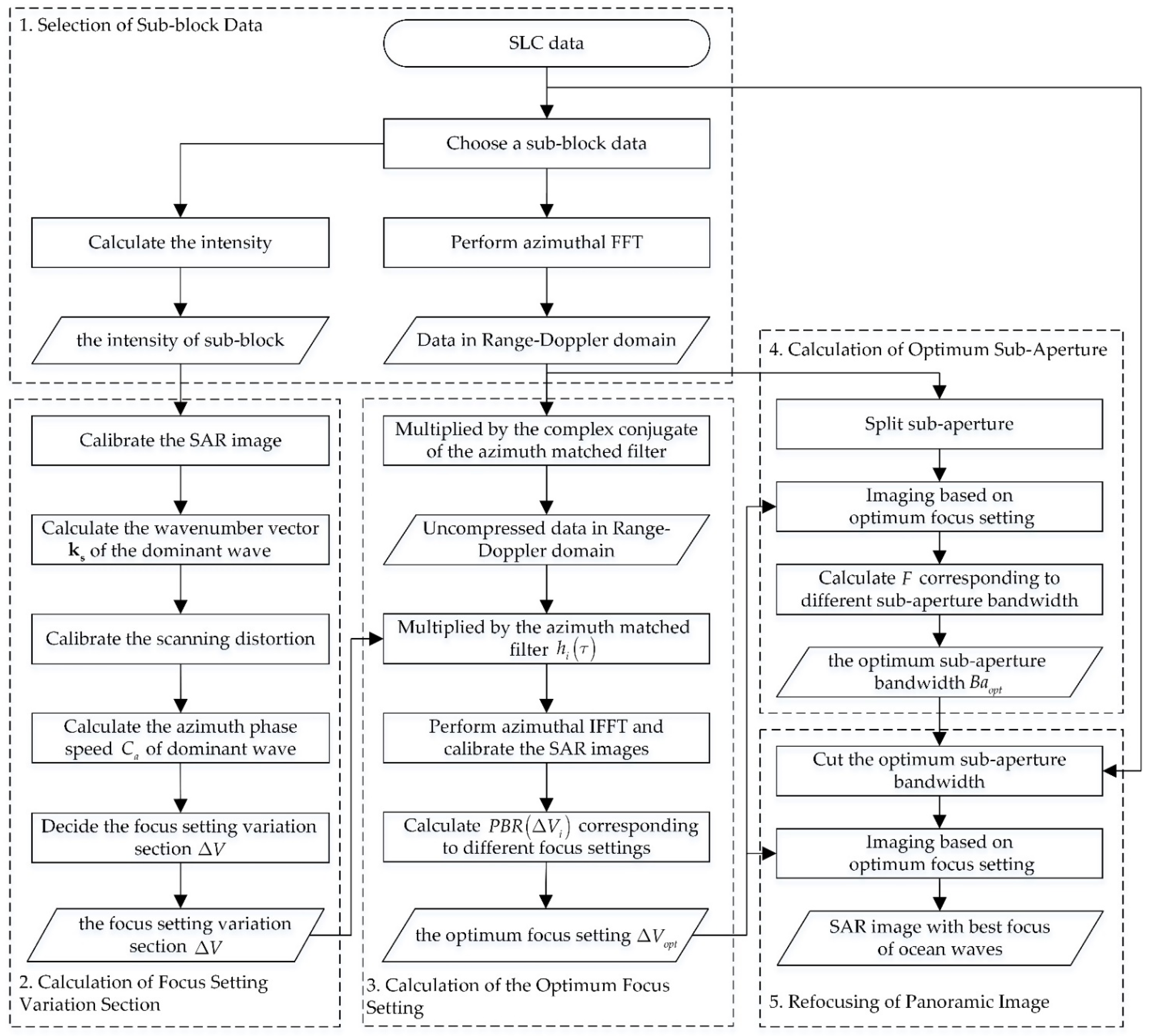
2. SAR Imaging Algorithm of Ocean Waves Based on Optimum Subaperture
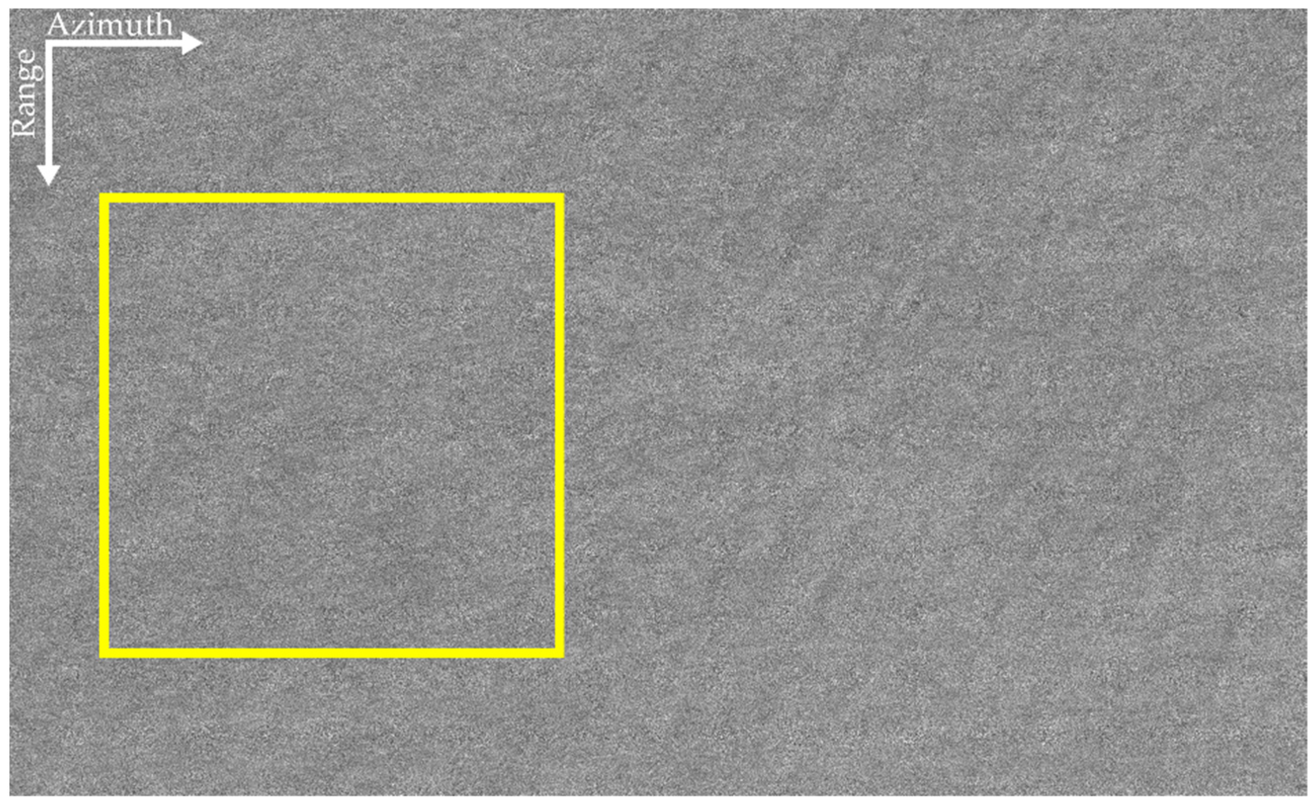
2.1. Selection of Sub-Block Data
2.2. Calculation of Focus Setting Variation Section
2.3. Calculation of the Optimum Focus Setting
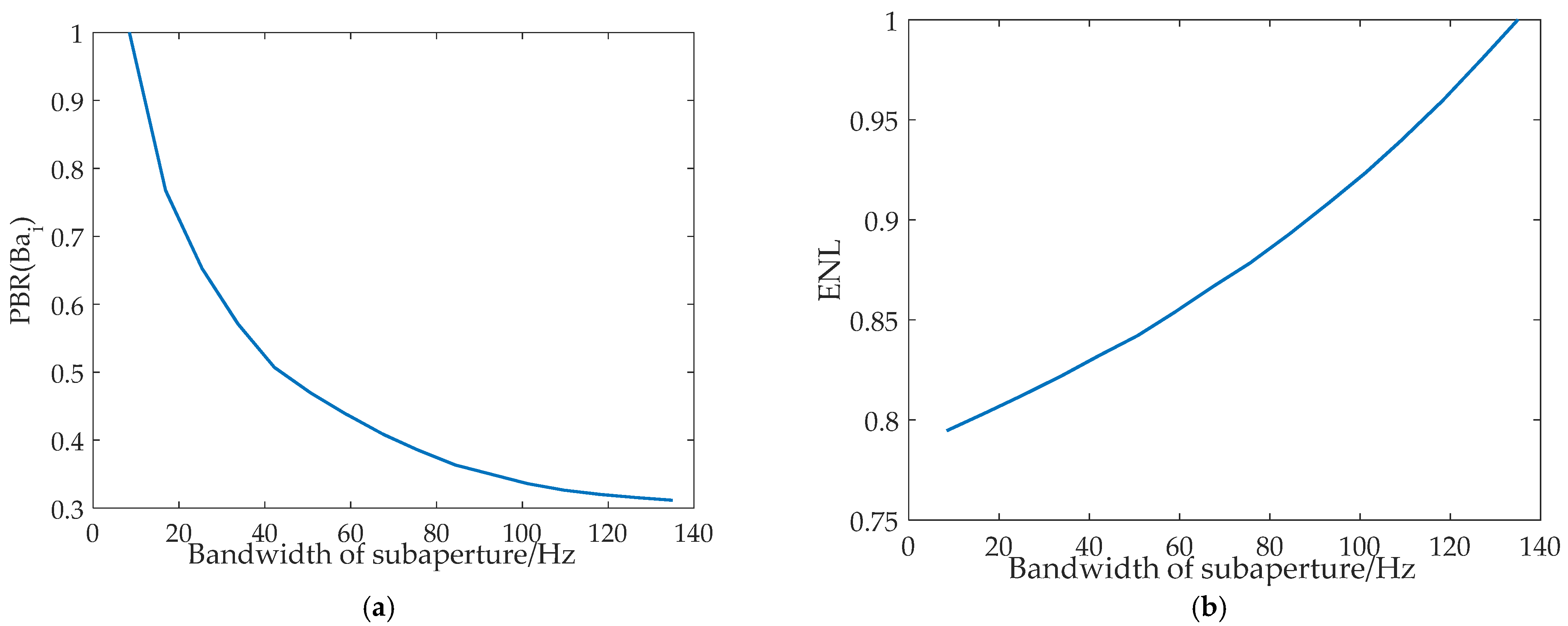
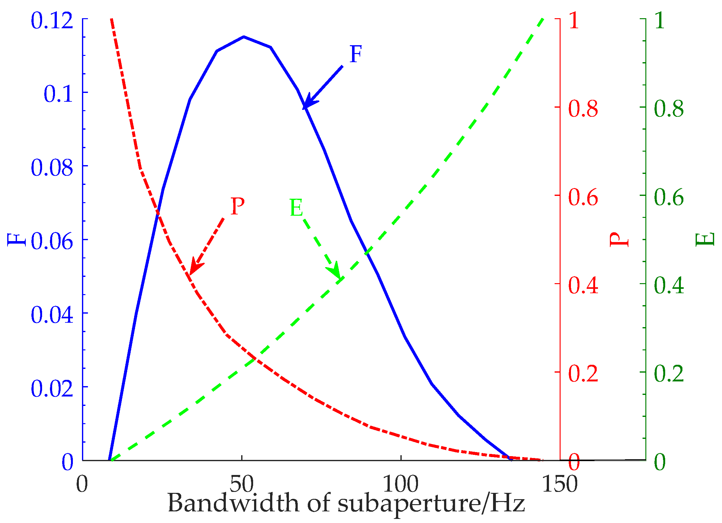
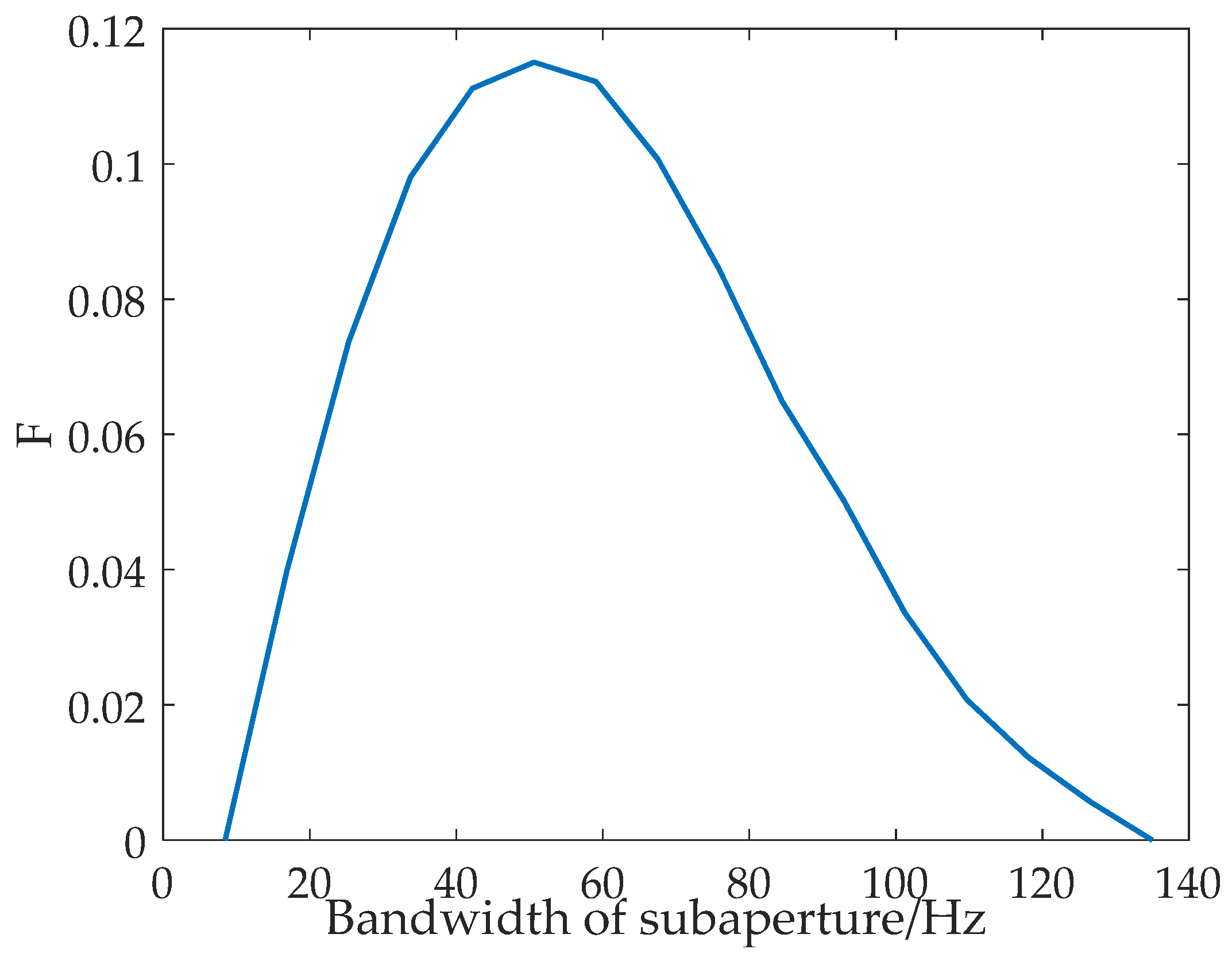
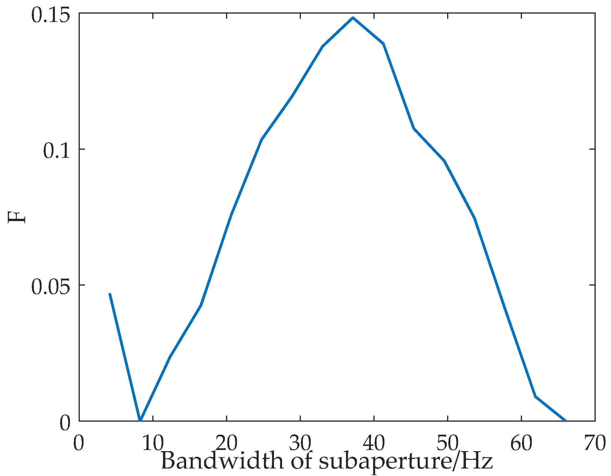
2.4. Calculation of Optimum Subaperture
2.5. Refocusing of Panoramic Image
3. Applying the Proposed Algorithm
3.1. Results of Airborne L-Band SAR Data Processing
3.2. Results of Airborne P-Band SAR Data Processing
4. Comparison and Quantitative Analysis of the Ocean Wave Refocusing Results
4.1. Comparison and Quantitative Analysis of the Ocean Wave Refocusing Results of Airborne L-Band SAR Data
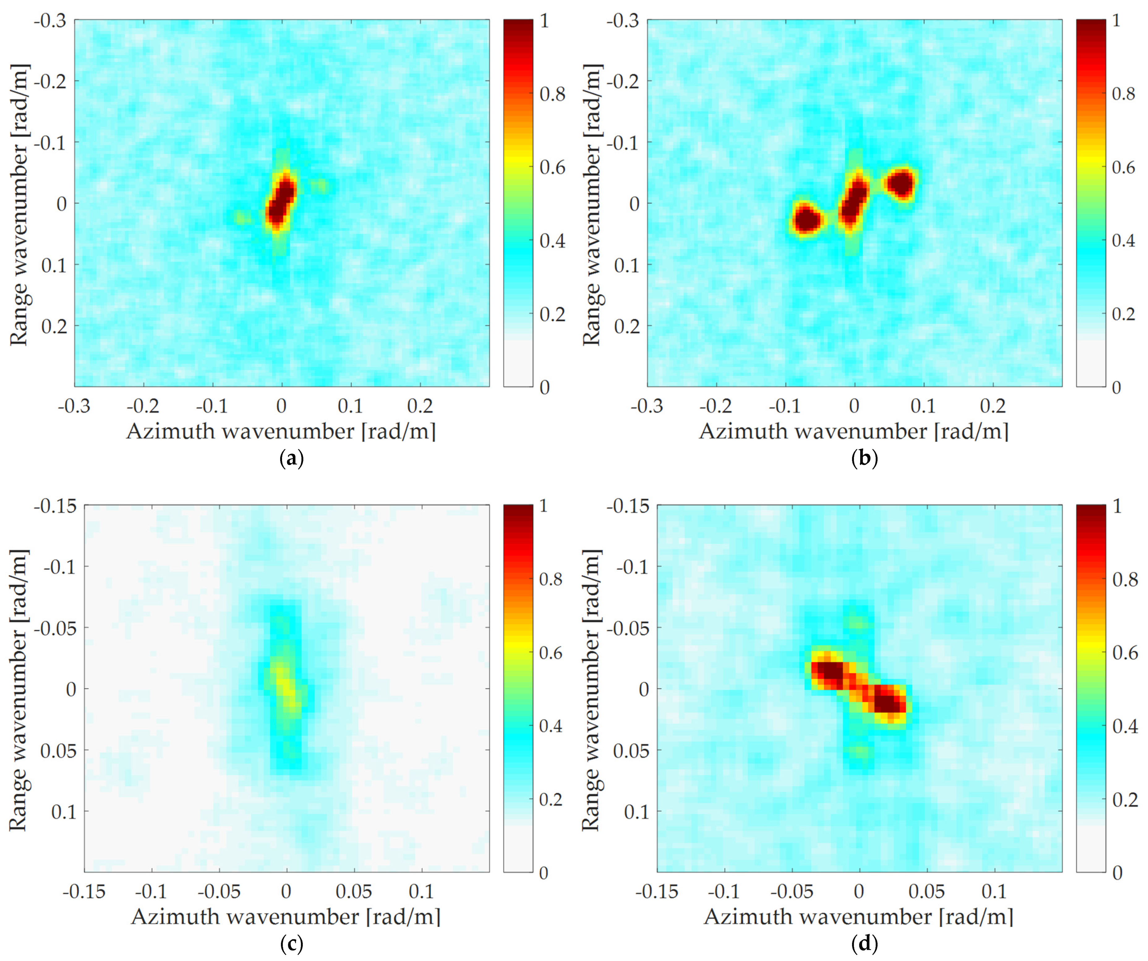
4.1.1. Comparison of the Ocean Wave Refocusing Results of Airborne L-Band SAR Data
4.1.2. Quantitative Analysis of the Ocean Wave Refocusing Results of Airborne L-Band SAR Data
- (1)
- Contrast of Images
- (2)
- Relative Normalized Modulation of Image Gray
- (3)
- Modulation Difference of Positive and Negative Gray
4.2. Comparison and Quantitative Analysis of the Ocean Wave Refocusing Results of Airborne P-Band SAR Data
4.2.1. Comparison of the Ocean Wave Refocusing Results of Airborne P-Band SAR Data
4.2.2. Quantitative Analysis of the Ocean Wave Refocusing Results of Airborne P-Band SAR Data
5. Discussion
5.1. Analysis of Algorithm Applicability
5.2. Prospects for Algorithm Applications
6. Conclusions
Author Contributions
Funding
Institutional Review Board Statement
Informed Consent Statement
Data Availability Statement
Acknowledgments
Conflicts of Interest
References
- Alpers, W.; Rufenach, C. The effect of orbital motions on synthetic aperture radar imagery of ocean waves. IEEE Trans. Antennas Propag. 1979, 27, 685–690. [Google Scholar] [CrossRef]
- Raney, R.K. Wave orbital velocity, fade, and sar response to azimuth waves. IEEE J. Ocean. Eng. 1981, 6, 140–146. [Google Scholar] [CrossRef]
- Stopa, J.E.; Ardhuin, F.; Chapron, B.; Collard, F. Estimating wave orbital velocity through the azimuth cutoff from space-borne satellites. J. Geophys. Res. Ocean. 2015, 120, 7616–7634. [Google Scholar] [CrossRef] [Green Version]
- Shao, W.; Zhang, Z.; Li, X.; Li, H. Ocean wave parameters retrieval from sentinel-1 sar imagery. Remote Sens. 2016, 8, 707. [Google Scholar] [CrossRef] [Green Version]
- Grieco, G.; Lin, W.; Migliaccio, M.; Nirchio, F.; Portabella, M. Dependency of the sentinel-1 azimuth wavelength cut-off on significant wave height and wind speed. Int. J. Remote Sens. 2016, 37, 5086–5104. [Google Scholar] [CrossRef]
- Stopa, J.E.; Mouche, A. Significant wave heights from sentinel-1 sar: Validation and applications. J. Geophys. Res. Ocean. 2017, 122, 1827–1848. [Google Scholar] [CrossRef] [Green Version]
- Du, Y.; Vachon, P.W.; Wolfe, J. Wind direction estimation from sar images of the ocean using wavelet analysis. Can. J. Remote Sens. 2002, 28, 498–509. [Google Scholar] [CrossRef]
- Horstmann, J.; Koch, W. Measurement of ocean surface winds using synthetic aperture radars. IEEE J. Ocean. Eng. 2006, 30, 508–515. [Google Scholar] [CrossRef]
- Lee, J.-S. Speckle suppression and analysis for synthetic aperture radar images. Opt. Eng. 1986, 25, 636–643. [Google Scholar] [CrossRef]
- Kuan, D.; Sawchuk, A.; Strand, T.; Chavel, P. Adaptive restoration of images with speckle. IEEE Trans. Acoust. Speech Signal Process. 1987, 35, 373–383. [Google Scholar] [CrossRef]
- Lu, C.; Li, W. Ship classification in high-resolution sar images via transfer learning with small training dataset. Sensors 2019, 19, 63. [Google Scholar] [CrossRef] [PubMed] [Green Version]
- Rostami, M.; Kolouri, S.; Eaton, E.; Kim, K. Deep transfer learning for few-shot sar image classification. Remote Sens. 2019, 11, 1374. [Google Scholar] [CrossRef] [Green Version]
- Wang, Z.; Du, L.; Mao, J.; Liu, B.; Yang, D. Sar target detection based on ssd with data augmentation and transfer learning. IEEE Geosci. Remote Sens. Lett. 2019, 16, 150–154. [Google Scholar] [CrossRef]
- Zhong, C.; Mu, X.; He, X.; Wang, J.; Zhu, M. Sar target image classification based on transfer learning and model compression. IEEE Geosci. Remote Sens. Lett. 2019, 16, 412–416. [Google Scholar] [CrossRef]
- Hamdi, I.; Tounsi, Y.; Benjelloun, M.; Nassim, A. Evaluation of the change in synthetic aperture radar imaging using transfer learning and residual network. Comput. Opt. 2021, 4, 600–607. [Google Scholar] [CrossRef]
- Hayt, D.W.; Alpers, W.; Burning, C.; Dewitt, R.; Henyey, F.; Kasilingam, D.P.; Keller, W.C.; Lyzenga, D.R.; Plant, W.J.; Schult, R.L. Focusing simulations of synthetic aperture radar ocean images. J. Geophys. Res. Ocean. 1990, 95, 16245–16261. [Google Scholar] [CrossRef]
- Kasilingam, D.P.; Hayt, D.W.; Shemdin, O.H. Focusing of synthetic aperture radar ocean images with long integration times. J. Geophys. Res. 1991, 96, 16935–16942. [Google Scholar] [CrossRef]
- Lyzenga, D.R. Numerical simulation of synthetic aperture radar image spectra for ocean waves. IEEE Trans. Geosci. Remote Sens. 1986, 24, 863–872. [Google Scholar] [CrossRef]
- Lyden, J.D.; Hammond, R.R.; Lyzenga, D.R.; Shuchman, R.A. Synthetic aperture radar imaging of surface ship wakes. J. Geophys. Res. 1988, 93, 12293. [Google Scholar] [CrossRef]
- Kasilingam, D.P.; Shemdin, O.H. Theory for synthetic aperture radar imaging of the ocean surface: With application to the tower ocean wave and radar dependence experiment on focus, resolution, and wave height spectra. J. Geophys. Res. 1988, 93, 13837–13848. [Google Scholar] [CrossRef]
- Raney, R.K.; Vachon, P.W. Synthetic aperture radar imaging of ocean waves from an airborne platform: Focus and tracking issues. J. Geophys. Res. Ocean. 1988, 93, 12475–12486. [Google Scholar] [CrossRef]
- Vachon, P.W.; Raney, R.K.; Emergy, W.J. A simulation for spaceborne sar imagery of a distributed, moving scene. IEEE Trans. Geosci. Remote Sens. 1989, 27, 67–78. [Google Scholar] [CrossRef]
- Shuchman, R.; Shemdin, O. Synthetic aperture radar imaging of ocean waves during the marineland experiment. IEEE J. Ocean. Eng. 1983, 8, 83–90. [Google Scholar] [CrossRef]
- Shemer, L. On the focusing of the ocean swell images produced by a regular and by an interferometric sar. Int. J. Remote Sens. 1995, 16, 925–947. [Google Scholar] [CrossRef]
- Wei, X.; Chong, J.; Zhao, Y.; Li, Y.; Yao, X. Airborne sar imaging algorithm for ocean waves based on optimum focus setting. Remote Sens. 2019, 11, 564. [Google Scholar] [CrossRef] [Green Version]
- Suchandt, S.; Romeiser, R. X-band sea surface coherence time inferred from bi-static sar interferometry. IEEE Trans. Geosci. Remote Sens. 2017, 55, 3941–3948. [Google Scholar] [CrossRef]
- Sjögren, T.K.; Vu, V.T.; Pettersson, M.I.; Wang, F.; Murdin, D.J.G.; Gustavsson, A.; Ulander, L.M.H. Suppression of clutter in multichannel sar gmti. IEEE Trans. Geosci. Remote Sens. 2014, 52, 4005–4013. [Google Scholar] [CrossRef]
- Moreira, A. Real-time synthetic aperture radar (sar) processing with a new subaperture approach. IEEE Trans. Geosci. Remote Sens. 1992, 30, 714–722. [Google Scholar] [CrossRef]
- Zeng, T.; Li, Y.; Ding, Z.; Long, T.; Yao, D.; Sun, Y. Subaperture approach based on azimuth-dependent range cell migration correction and azimuth focusing parameter equalization for maneuvering high-squint-mode sar. IEEE Trans. Geosci. Remote Sens. 2015, 53, 6718–6734. [Google Scholar] [CrossRef]
- Yeo, T.S.; Tan, N.L.; Zhang, C.B.; Lu, Y.H. A new subaperture approach to high squint sar processing. IEEE Trans. Geosci. Remote Sens. 2001, 39, 954–968. [Google Scholar]
- Tajirian, E.K. Multifocus processing of l band synthetic aperture radar images of ocean waves obtained during the tower ocean wave and radar dependence experiment. J. Geophys. Res. Ocean. 1988, 93, 13849–13857. [Google Scholar] [CrossRef]
- Vachon, P.; Krogstad, H.; Scottpaterson, J. Airborne and spaceborne synthetic aperture radar observations of ocean waves. Atmosphere 1994, 32, 83–112. [Google Scholar] [CrossRef]
- Hwang, P.A.; Toporkov, J.V.; Sletten, M.A.; Menk, S.P. Mapping surface currents and waves with interferometric synthetic aperture radar in coastal waters: Observations of wave breaking in swell-dominant conditions. J. Phys. Oceanogr. 2012, 43, 563–582. [Google Scholar] [CrossRef]
- Jain, A.; Shemdin, O. L band sar ocean wave observations during marsen. J. Geophys. Res. Ocean. 1983, 88, 9792–9808. [Google Scholar] [CrossRef]
- Ferro-Famil, L.; Reigber, A.; Pottier, E.; Boerner, W. Scene characterization using subaperture polarimetric sar data. IEEE Trans. Geosci. Remote Sens. 2003, 41, 2264–2276. [Google Scholar] [CrossRef]
- Lay-Ekuakille, A.; Ugwiri, M.A.; Okitadiowo, J.P.D.; Telesca, V.; Picuno, P.; Liguori, C.; Singh, S. Sar sensors measurements for environmental classification: Machine learning-based performances. IEEE Instrum. Meas. Mag. 2020, 23, 23–30. [Google Scholar] [CrossRef]
- Fang, S.; Tan, Y.; Zhang, T.; Xu, Z.; Liu, H. Effective prediction of bug-fixing priority via weighted graph convolutional networks. IEEE Trans. Reliab. 2021, 70, 563–574. [Google Scholar] [CrossRef]


| Parametric Name | Parametric Symbol | Parametric Value | |
|---|---|---|---|
| L-Band | P-Band | ||
| Radar wavelength (m) | 0.23 | 0.5 | |
| Pulse length (us) | 5.4 | 3 | |
| Radar bandwidth (MHz) | 125 | 160 | |
| PRF (Hz) | 900 | 1000 | |
| Platform speed (m/s) | 132 | 134 | |
| Platform height (m) | 8100 | 8600 | |
| Slant range of scene center (m) | 13,000 | 11,300 | |
| Doppler bandwidth (Hz) | 66 | 135 | |
| SAR integration time (s) | 7 | 21 | |
| Data | 13 September 2014 | 11 October 2014 |
| Corresponding SAR data | L-band data | P-band data |
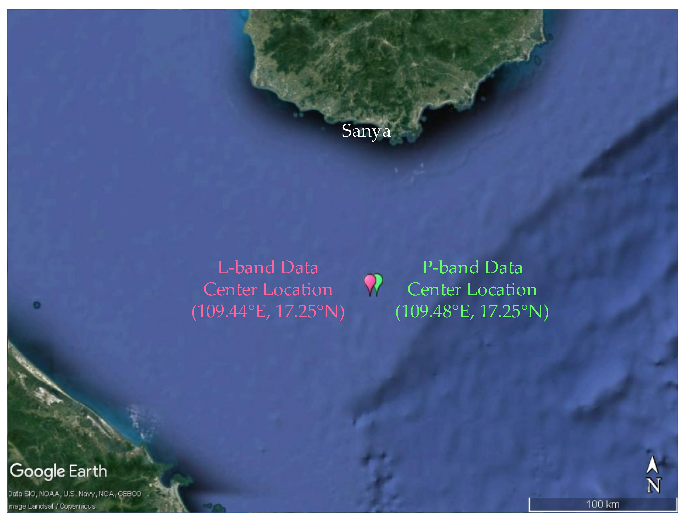
| Central location of SAR data | (109.44° E, 17.25° N) | (109.48° E, 17.25° N) |
| 10 m wind speed (m/s) | 3 | 6.5 |
| Significant wave height (m) | 0.5 | 1.5 |
| Mean wave period (s) | 5 | 8.5 |
| Mean wave direction * (deg) | 158 | 30 |
| Original Image | Result Based on Half of Azimuth Phase Speed | Result Based on Optimum Focus Setting | Result of the Proposed Algorithm | |
|---|---|---|---|---|
| 0.5791 | 1.0306 | 1.0434 | 1.1654 | |
| 0.2272 | 0.4075 | 0.4124 | 0.4726 | |
| 0.1427 | 0.2532 | 0.2562 | 0.2938 |
| Original Image | Result Based on Half of Azimuth Phase Speed | Result Based on Optimum Focus Setting | Result of the Proposed Algorithm | |
|---|---|---|---|---|
| 0.3412 | 0.6096 | 0.6279 | 0.8770 | |
| 0.1353 | 0.2443 | 0.2512 | 0.3526 | |
| 0.0847 | 0.1489 | 0.1533 | 0.2143 |
Publisher’s Note: MDPI stays neutral with regard to jurisdictional claims in published maps and institutional affiliations. |
© 2022 by the authors. Licensee MDPI, Basel, Switzerland. This article is an open access article distributed under the terms and conditions of the Creative Commons Attribution (CC BY) license (https://creativecommons.org/licenses/by/4.0/).
Share and Cite
Zhao, Y.; Wei, X.; Chong, J.; Diao, L. SAR Imaging Algorithm of Ocean Waves Based on Optimum Subaperture. Sensors 2022, 22, 1299. https://doi.org/10.3390/s22031299
Zhao Y, Wei X, Chong J, Diao L. SAR Imaging Algorithm of Ocean Waves Based on Optimum Subaperture. Sensors. 2022; 22(3):1299. https://doi.org/10.3390/s22031299
Chicago/Turabian StyleZhao, Yawei, Xianen Wei, Jinsong Chong, and Lijie Diao. 2022. "SAR Imaging Algorithm of Ocean Waves Based on Optimum Subaperture" Sensors 22, no. 3: 1299. https://doi.org/10.3390/s22031299
APA StyleZhao, Y., Wei, X., Chong, J., & Diao, L. (2022). SAR Imaging Algorithm of Ocean Waves Based on Optimum Subaperture. Sensors, 22(3), 1299. https://doi.org/10.3390/s22031299