
Vehicle Bump Testing Parameters Influencing Modal Identification of Long-Span Segmental Prestressed Concrete Bridges


Abstract
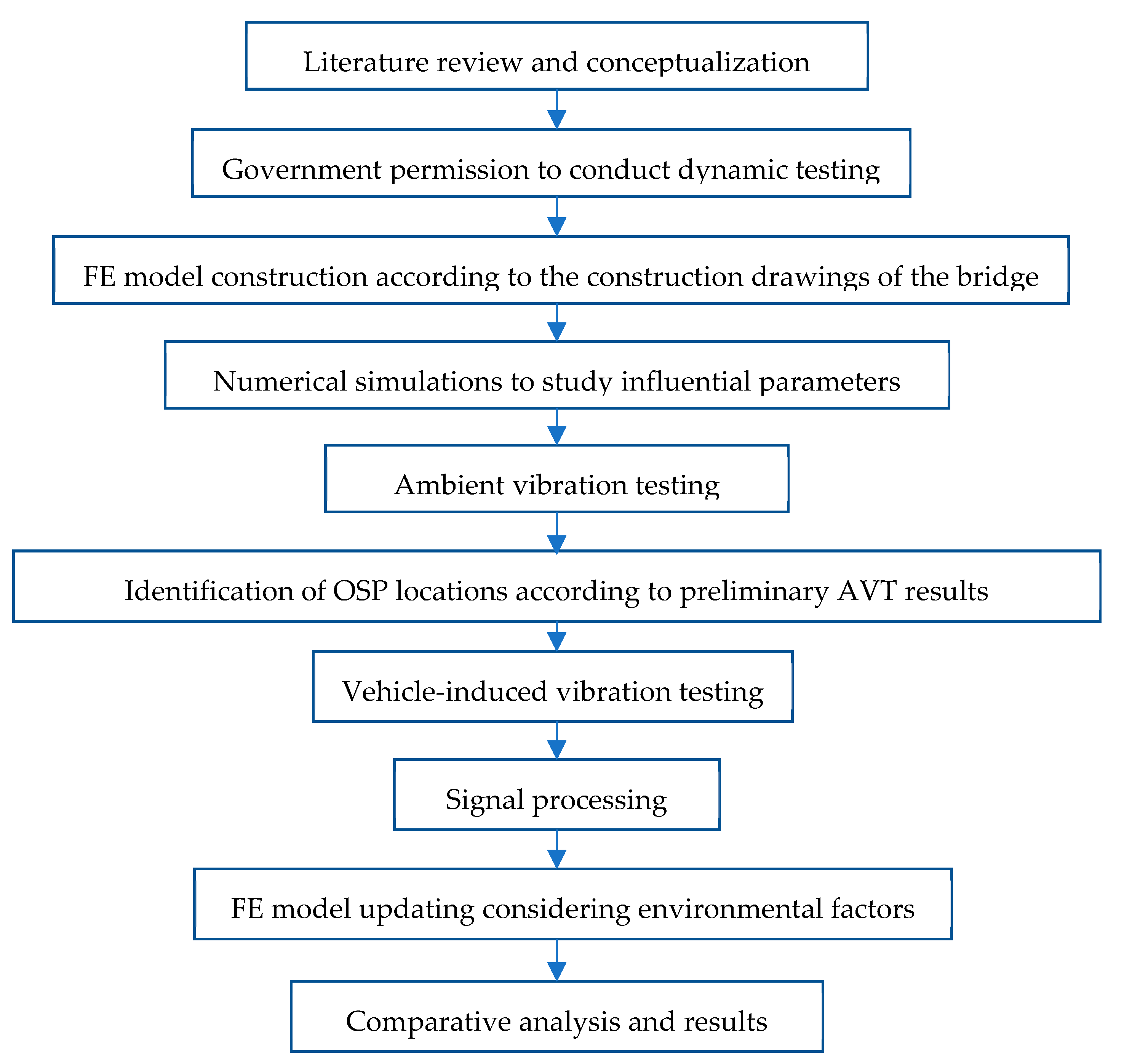
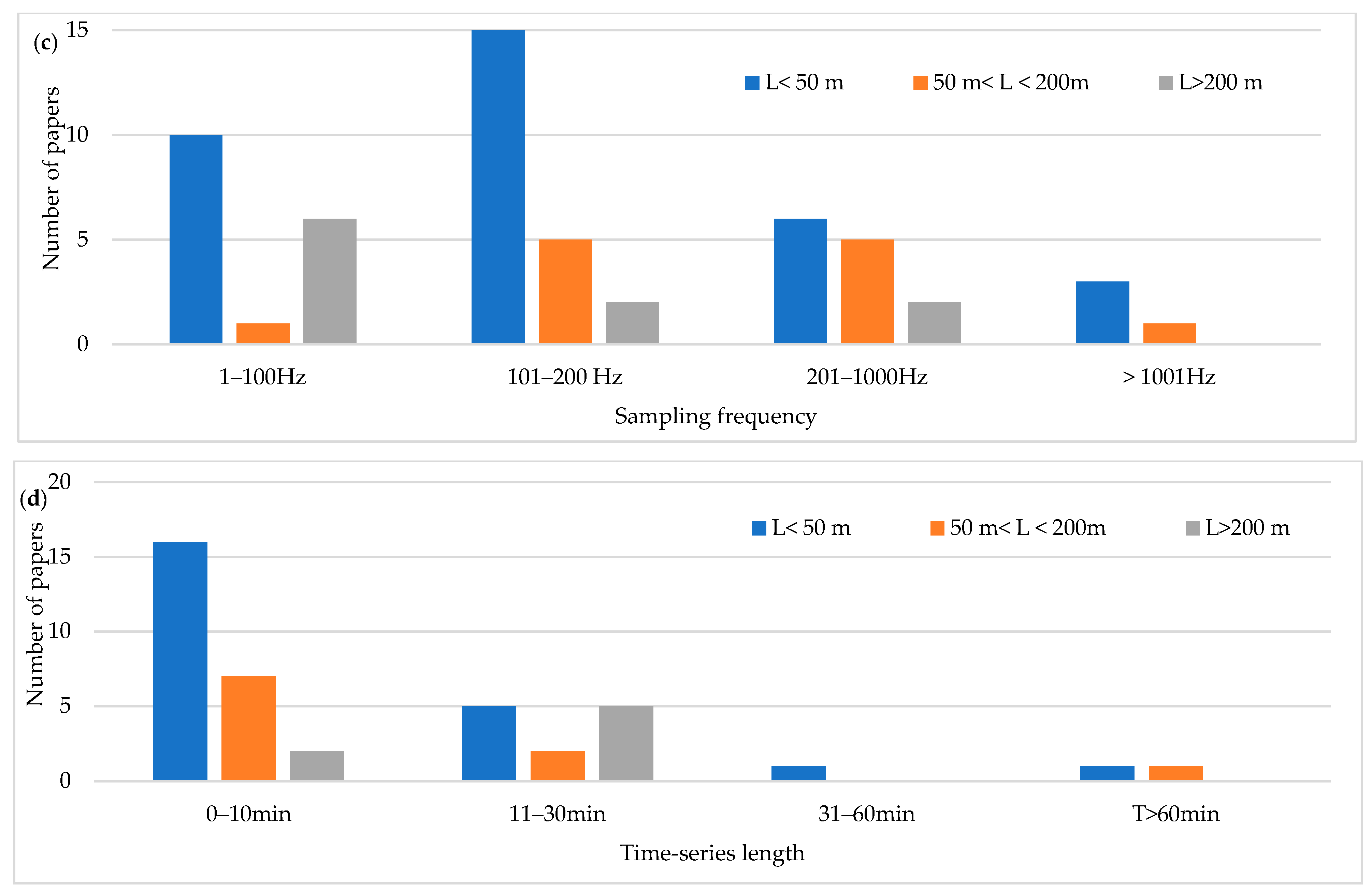
:1. Introduction
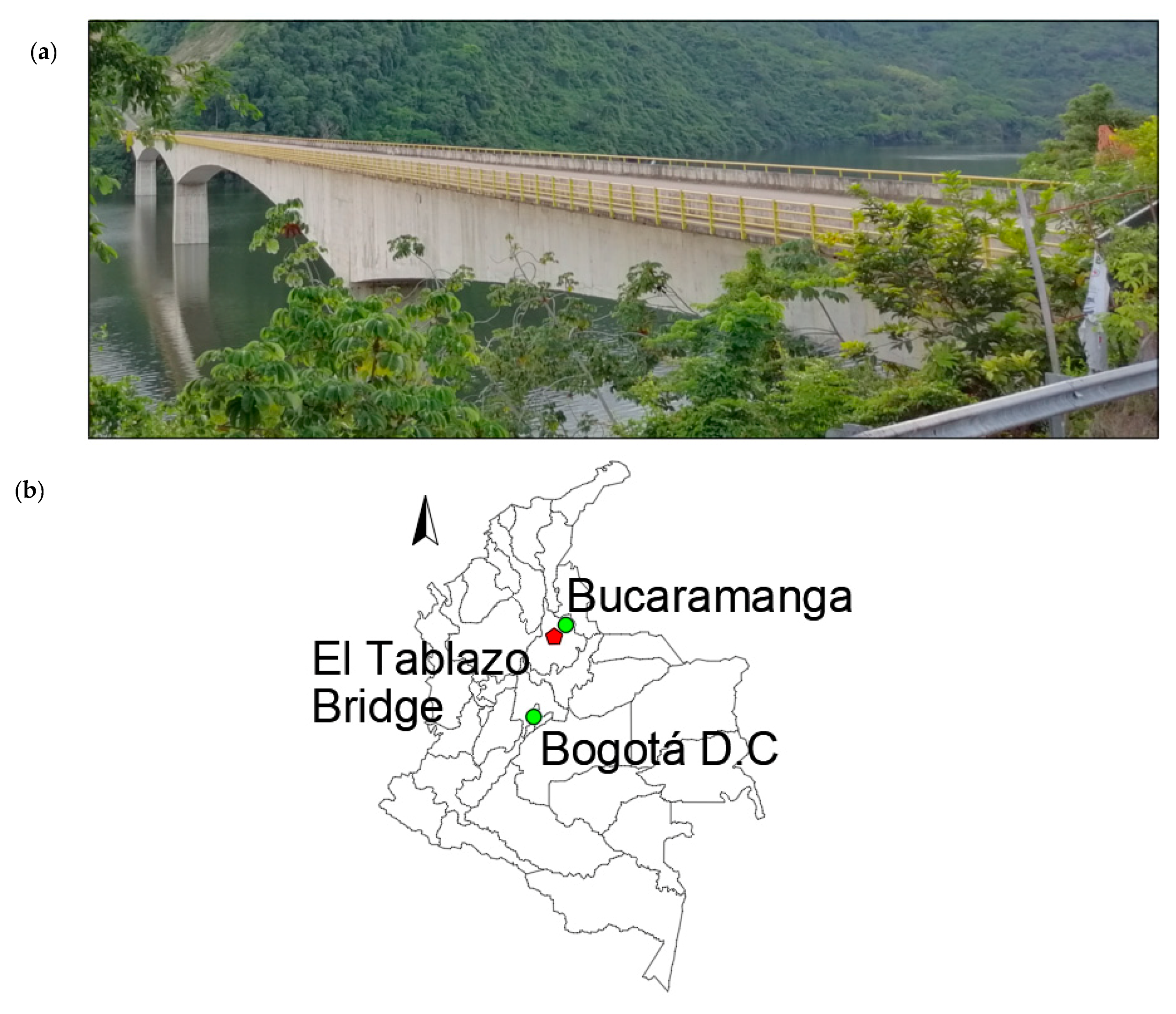
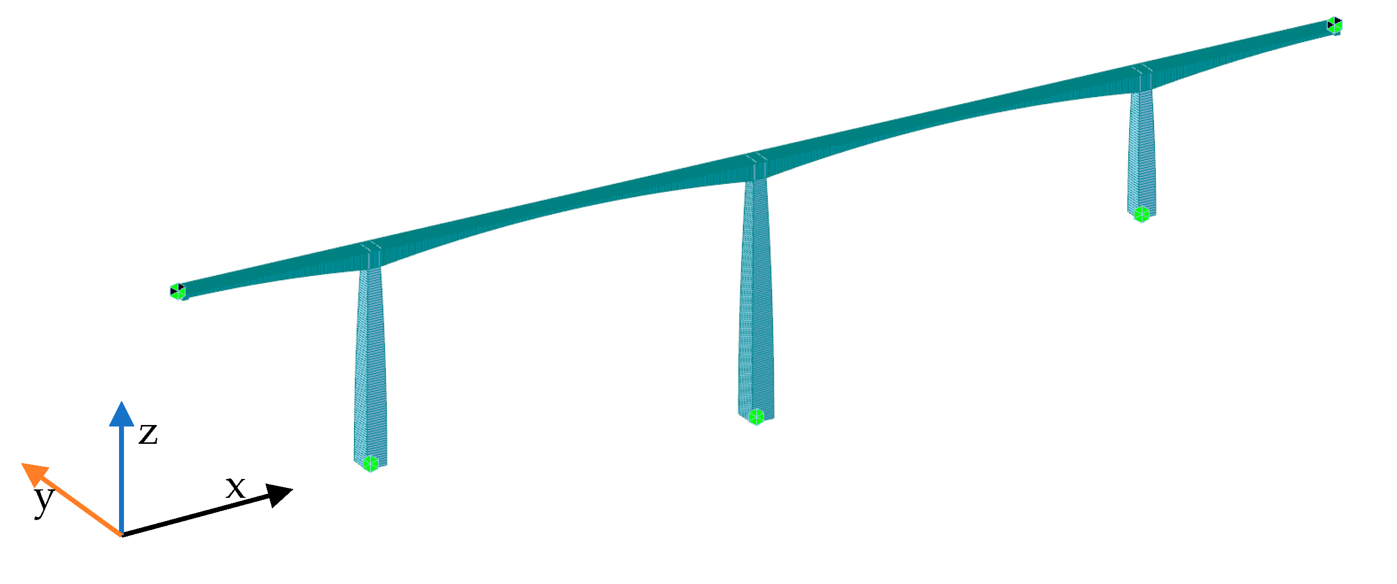
2. Study Case: The Tablazo Bridge
3. Preliminary Analysis for Influential Parameters
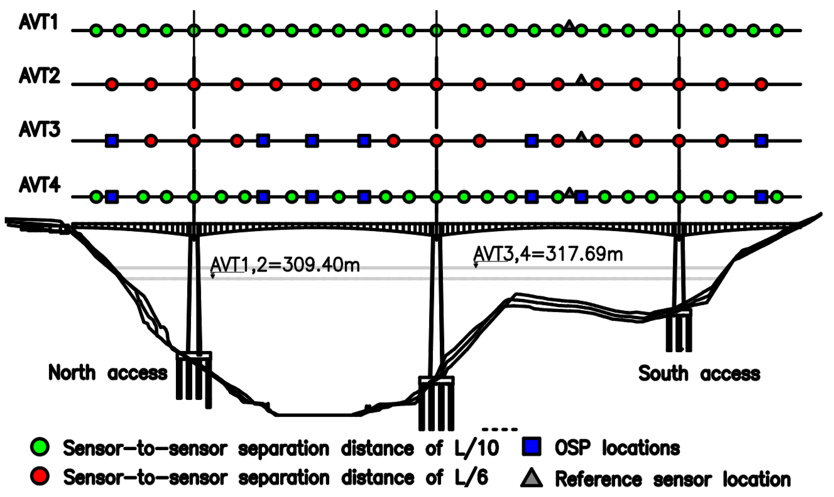
4. Ambient Vibration Tests
5. Vehicle-Induced Excitation Tests
6. Comparisons
- The incidence of sensor location in AVTs with full time-series length.
- The incidence of time-series length in AVTs by equaling time-series length to 20 min.
- The incidence of excitation source between AVTs and VITs with full time-series length.
- The incidence of OSP in VITs with respect to AVTs with full time-series length.
- The incidence of AVTs with time-series length equals to VITs (10 min).
- The cost comparison between both types of dynamic tests.
6.1. FE Model Updating
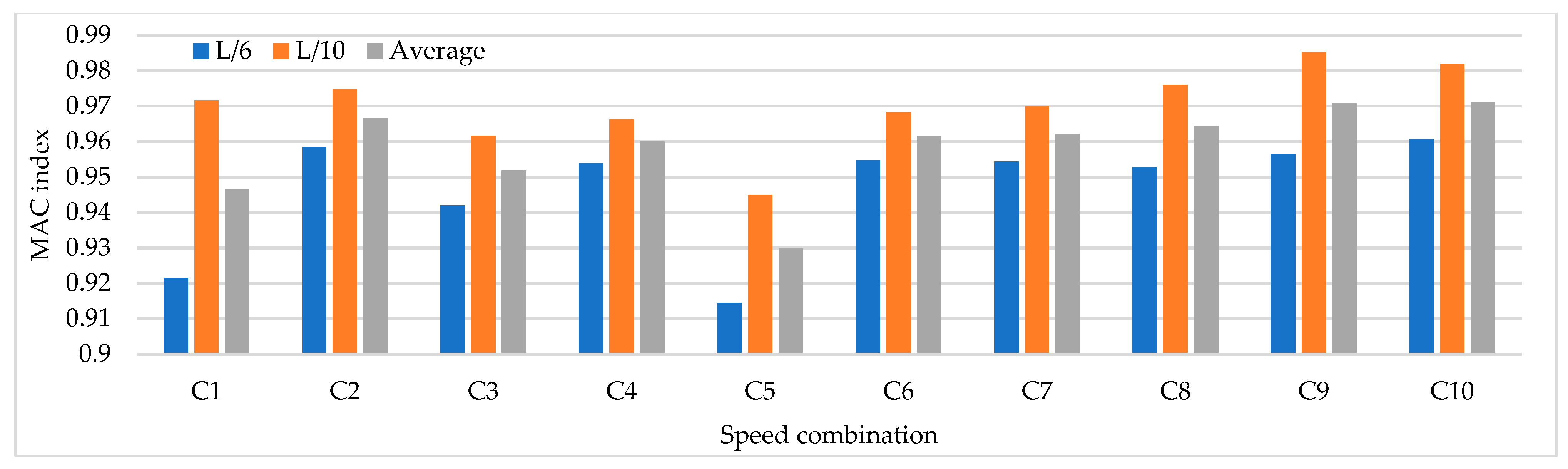
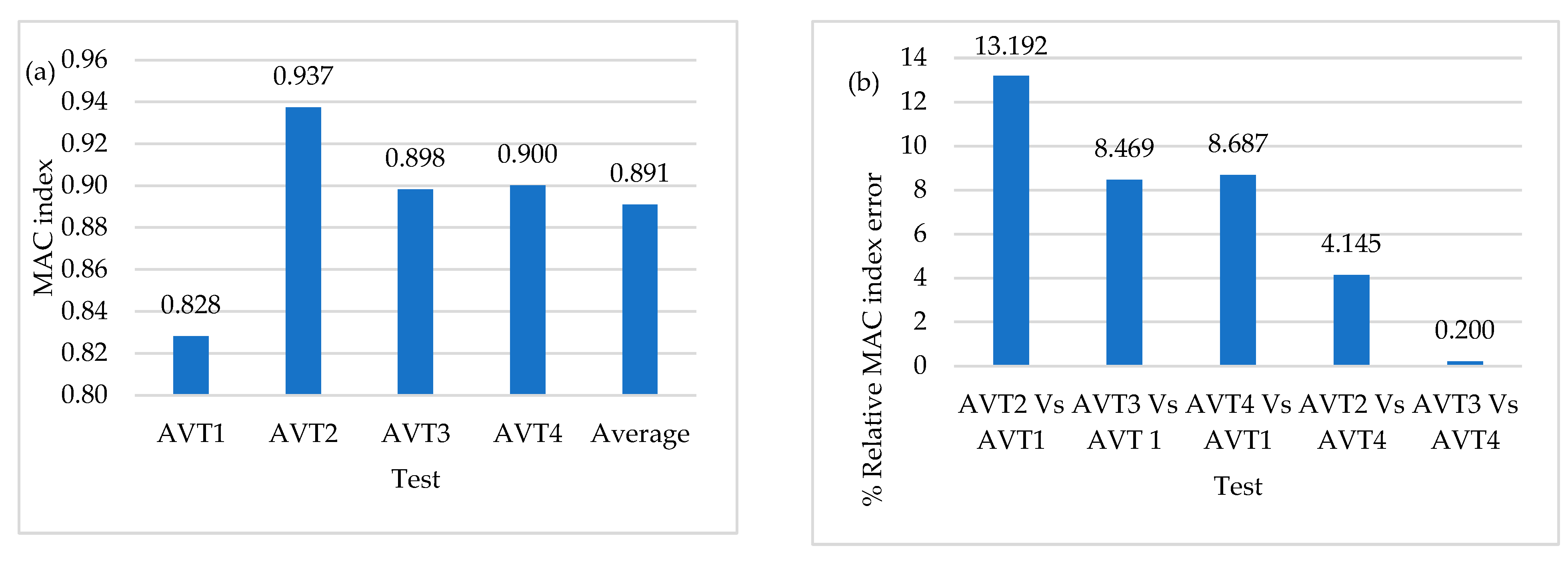
6.2. The Incidence of Sensor Location in AVTs with Full Time-Series Length
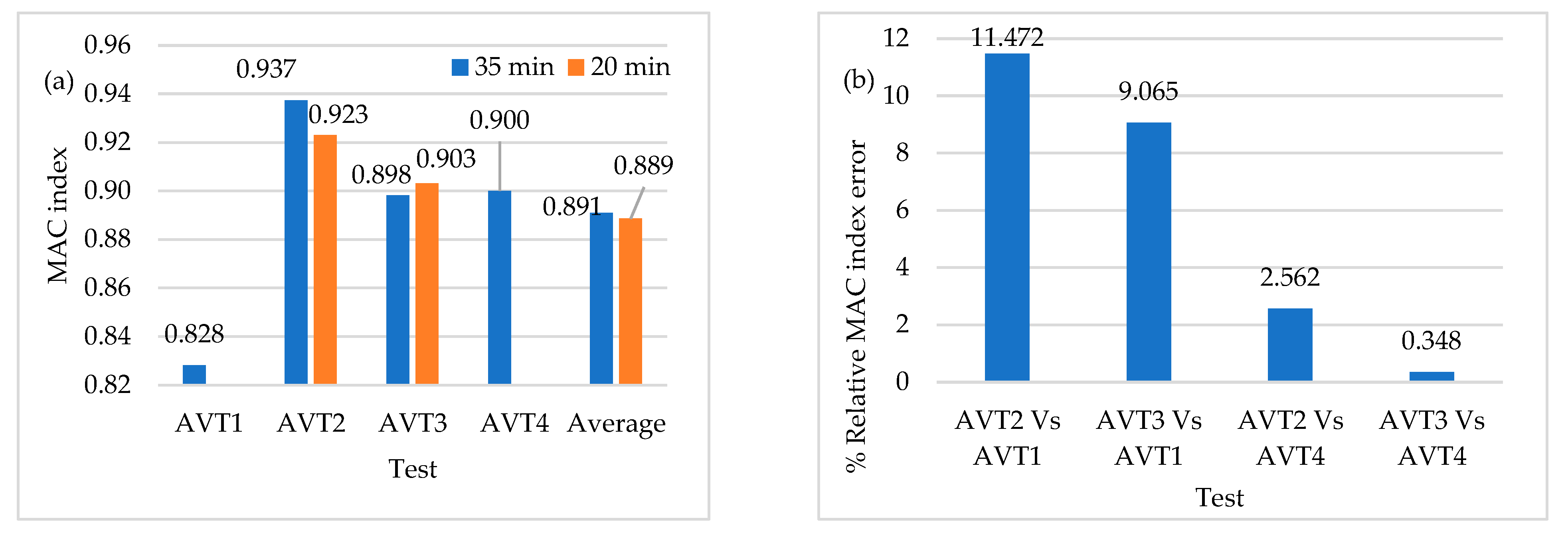
6.3. The Incidence of Time-Series Length in AVTs and Adjusted Time-Series Length to 20 min
6.4. The Incidence of Excitation Source between AVTs and VITs with Full Time-Series Length
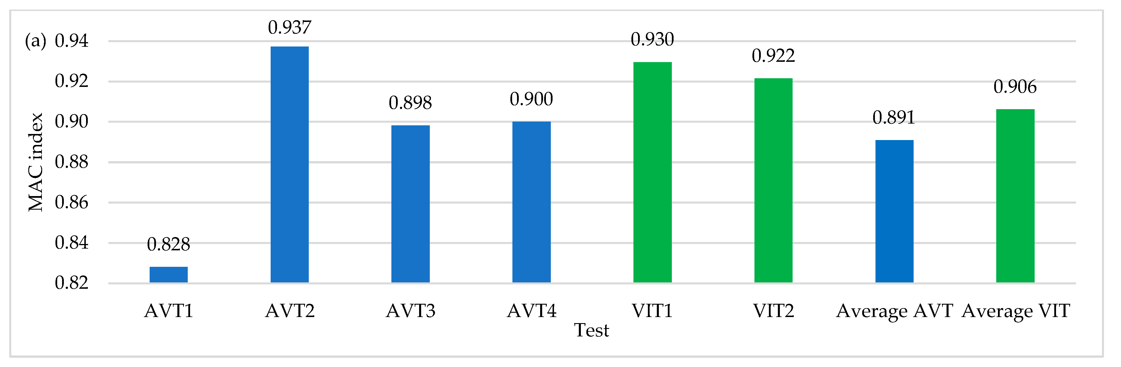
6.5. The Incidence of OSP in VITs with Respect to AVTs with Full Time-Series Length
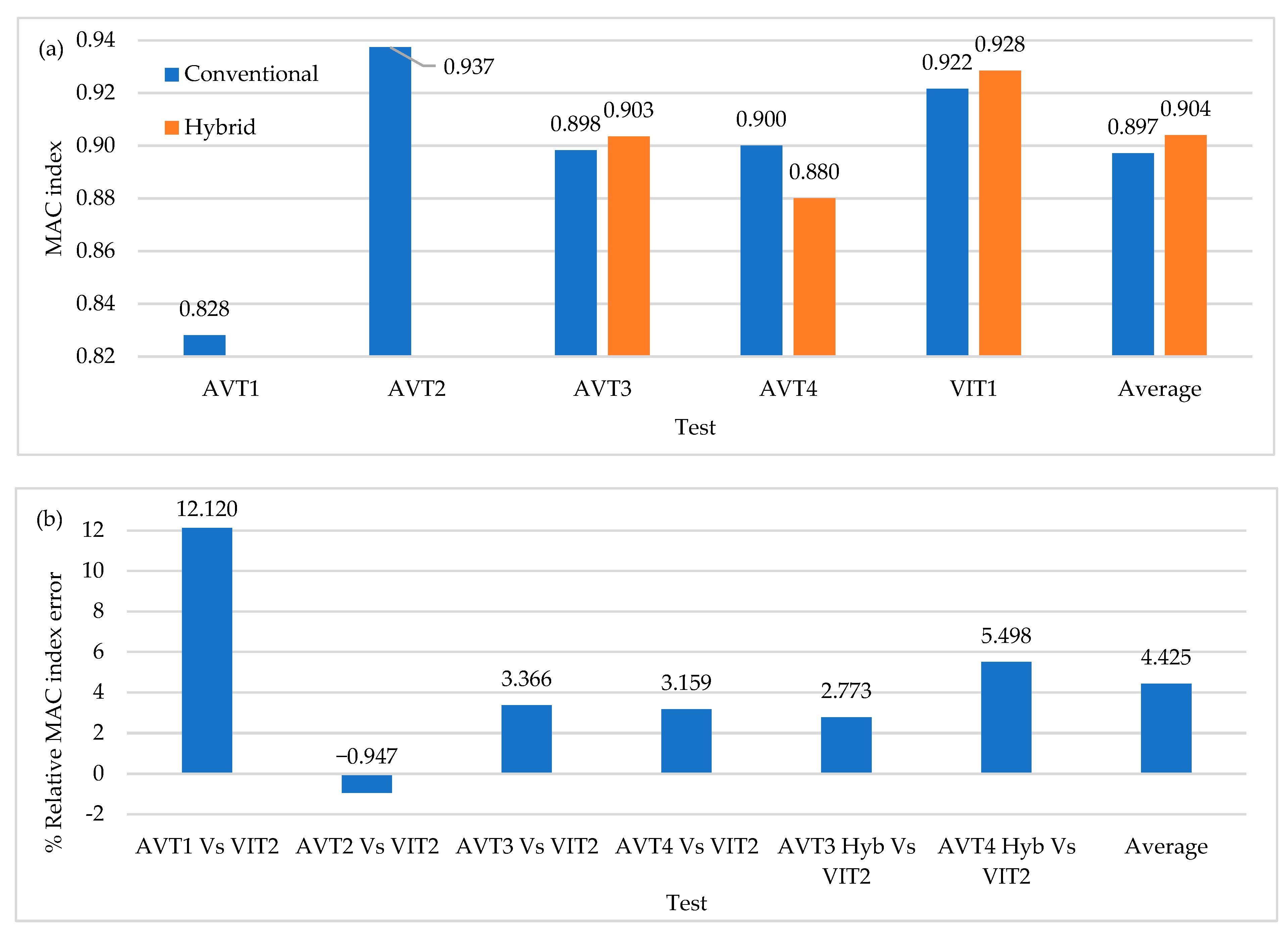
6.6. The Incidence of AVTs with Time-Series Length Equals to VITs’ Time-Series Length (10 min)
6.7. Cost Comparison
7. Conclusions
Author Contributions
Funding
Institutional Review Board Statement
Informed Consent Statement
Data Availability Statement
Acknowledgments
Conflicts of Interest
References
- Ye, X.; Chen, X.; Lei, Y.; Fan, J.; Mei, L. An Integrated Machine Learning Algorithm for Separating the Long-Term Deflection Data of Prestressed Concrete Bridges. Sensors 2018, 18, 4070. [Google Scholar] [CrossRef] [PubMed] [Green Version]
- Ko, J.M.; Ni, Y.-Q. Technology developments in structural health monitoring of large-scale bridges. Eng. Struct. 2005, 27, 1715–1725. [Google Scholar] [CrossRef]
- Catbas, F.N.; Susoy, M.; Frangopol, D.M. Structural health monitoring and reliability estimation: Long span truss bridge application with environmental monitoring data. Eng. Struct. 2008, 30, 2347–2359. [Google Scholar] [CrossRef]
- Sun, L.; Shang, Z.; Xia, Y.; Bhowmick, S.; Nagarajaiah, S. Review of Bridge Structural Health Monitoring Aided by Big Data and Artificial Intelligence: From Condition Assessment to Damage Detection. J. Struct. Eng. 2020, 146, 04020073. [Google Scholar] [CrossRef]
- Hu, W.-H.; Tang, D.-H.; Teng, J.; Said, S.; Rohrmann, R.G. Structural Health Monitoring of a Prestressed Concrete Bridge Based on Statistical Pattern Recognition of Continuous Dynamic Measurements over 14 years. Sensors 2018, 18, 4117. [Google Scholar] [CrossRef] [PubMed] [Green Version]
- Xu, Y.; Brownjohn, J.; Huseynov, F. Accurate Deformation Monitoring on Bridge Structures Using a Cost-Effective Sensing System Combined with a Camera and Accelerometers: Case Study. J. Bridg. Eng. 2019, 24, 05018014. [Google Scholar] [CrossRef] [Green Version]
- Rizzo, P.; Enshaeian, A. Challenges in Bridge Health Monitoring: A Review. Sensors 2021, 21, 4336. [Google Scholar] [CrossRef]
- Tan, G.; Kong, Q.; Wu, C.; Wang, S.; Ma, G. Analysis method of dynamic response in the whole process of the vehicle bump test of simply supported bridge. Adv. Mech. Eng. 2019, 11. [Google Scholar] [CrossRef]
- Zhang, Q.; Hou, J.; Jankowski, Ł. Bridge Damage Identification Using Vehicle Bump Based on Additional Virtual Masses. Sensors 2020, 20, 394. [Google Scholar] [CrossRef] [Green Version]
- Gatti, M. Structural health monitoring of an operational bridge: A case study. Eng. Struct. 2019, 195, 200–209. [Google Scholar] [CrossRef]
- Asociación Colombiana de Ingeniería Sísmica. SECCIÓN 4: Análisis y evaluación structural. In Norma Colombiana de Diseño de Puentes, CCP 14, 1st ed.; Asociación Colombiana de Ingeniería Sísmica: Bogota, Colombia, 2014; p. 83. [Google Scholar]
- Barthorpe, R.J.; Worden, K. Emerging Trends in Optimal Structural Health Monitoring System Design: From Sensor Placement to System Evaluation. J. Sens. Actuator Networks 2020, 9, 31. [Google Scholar] [CrossRef]
- Salawu, O.S.; Williams, C. Bridge Assessment Using Forced-Vibration Testing. J. Struct. Eng. 1995, 121, 161–173. [Google Scholar] [CrossRef]
- Salawu, O.S. Assessment of bridges: Use of dynamic testing. Can. J. Civ. Eng. 1997, 24, 218–228. [Google Scholar] [CrossRef]
- Ortiz, O.; Patrón, A.; Reyes, E.; Robles, V.; Ruiz-Sandoval, M.E.; Cremona, C. Evaluación De La Capacidad De Carga Del Puente Antonio Dovalí Jaime, Mediante El Uso De Pruebas De Carga Estáticas Y Dinámicas. Concreto Cemento. Investig. Desarro. 2010, 2, 31–43. [Google Scholar]
- Brownjohn, J.M.W.; A Dumanoglu, A.; Severn, R.T.; A Taylor, C.; Littler, J.D.; Maguire, J.R. Discussion. Ambient Vibration Measurements Of The Humber Suspension Bridge and Com Parsions with Calculated Characteristics. Proc. Inst. Civ. Eng. 1988, 85, 725–730. [Google Scholar] [CrossRef] [Green Version]
- Brownjohn, J.; Magalhaes, F.; Caetano, E.; Cunha, A. Ambient vibration re-testing and operational modal analysis of the Humber Bridge. Eng. Struct. 2010, 32, 2003–2018. [Google Scholar] [CrossRef] [Green Version]
- Magalhães, F.; Caetano, E.; Cunha, Á; Flamand, O.; Grillaud, G. Ambient and free vibration tests of the Millau Viaduct: Evaluation of alternative processing strategies. Eng. Struct. 2012, 45, 372–384. [Google Scholar] [CrossRef]
- Tian, Y.; Zhang, J.; Xia, Q.; Li, P. Flexibility identification and deflection prediction of a three-span concrete box girder bridge using impacting test data. Eng. Struct. 2017, 146, 158–169. [Google Scholar] [CrossRef]
- Reynolds, P.; Pavic, A. Comparison of forced and ambient vibration measurements on a bridge. In Proceedings of the International Modal Analysis Conference—IMAC, Kissimmee, Florida, USA, 5–8 February 2001; Volume 1, pp. 846–851. [Google Scholar]
- Sahin, A.; Bayraktar, A. Forced-Vibration Testing and Experimental Modal Analysis of a Steel Footbridge for Structural Identification. J. Test. Evaluation 2014, 42, 20130166. [Google Scholar] [CrossRef]
- Pachón, P.; Castro, R.; García, M.E.P.; Compán, V.; Puertas, E.E. Torroja’s bridge: Tailored experimental setup for SHM of a historical bridge with a reduced number of sensors. Eng. Struct. 2018, 162, 11–21. [Google Scholar] [CrossRef]
- Cunha, Á.; Caetano, E. From input-Output to Output-Only modal identification of civil engineering struct. In Proceedings of the 1st International Operational Modal Analysis Conference, IOMAC, Copenhagen, Denmark, 26–27 April 2005. [Google Scholar]
- Cantieni, R. Experimental methods used in system identification of civil engineering structures. In Proceedings of the 1st International Operational Modal Analysis Conference, IOMAC, Copenhagen, Denmark, 26–27 April 2005. [Google Scholar]
- Yang, Y.; Zhang, B.; Wang, T.; Xu, H.; Wu, Y. Two-axle test vehicle for bridges: Theory and applications. Int. J. Mech. Sci. 2019, 152, 51–62. [Google Scholar] [CrossRef]
- Valdés, J.; La Colina, J.D. Análisis de la amplificación dinámica de la carga viva en puentes con base en pruebas experimentales. Rev. Tecnol.-ESPOL 2008, 21, 149–156. [Google Scholar]
- Cantieni, R. Dynamic Load Tests on Highway Bridges in Switzerland—60 Years of Experience; Swiss Federal Laboratories for Materials Testing and Research: Dübendorf, Switzerland, 1983; Volume 211. [Google Scholar]
- Gao, Q.F.; Wang, Z.L.; Li, J.; Chen, C.; Jia, H.Y. Dynamic load allowance in different positions of the multi-span girder bridge with variable cross-section. J. Vibroeng. 2015, 17, 2025–2039. [Google Scholar]
- Cantero, D.; McGetrick, P.; Kim, C.-W.; Obrien, E. Experimental monitoring of bridge frequency evolution during the passage of vehicles with different suspension properties. Eng. Struct. 2019, 187, 209–219. [Google Scholar] [CrossRef]
- Dirección General de Carreteras. Recomendaciones para la Realización de Pruebas de Carga de Recepción en Puentes de Carretera, Primera; Centro de Publicaciones: Madrid, Spain, 1999; Volume 1. [Google Scholar] [CrossRef]
- Service d’Etudes techniques des Routes et Autoroutes. Technical Guide Loading Tests on Road Bridges and Footbridges, 1st ed.; SETRA: Bagneux, France, 2006; Available online: http://www.setra.equipement.gouv.fr (accessed on 10 June 2020).
- Burdet, O.; Corthay, S. Dynamic load testing of Swiss bridges. In Proceedings of the IABSE Symposium San Francisco, Extending the Lifespan of Structures, San Francesco, CA, USA, 23–25 August 1995; Volume 73, pp. 1123–1128. Available online: http://is-beton.epfl.ch//Publications/199x/Burdet95.pdf (accessed on 6 September 2020).
- Conte, J.P.; He, X.; Moaveni, B.; Masri, S.F.; Caffrey, J.P.; Wahbeh, M.; Tasbihgoo, F.; Whang, D.H.; Elgamal, A. Dynamic Testing of Alfred Zampa Memorial Bridge. J. Struct. Eng. 2008, 134, 1006–1015. [Google Scholar] [CrossRef] [Green Version]
- Argentini, T.; Belloli, M.; Rosa, L.; Sabbioni, E.; Zasso, A.; Villani, M. Modal Identification of a Cable-Stayed Bridge by Means of Truck Induced Vibrations. In Topics on the Dynamics of Civil Structures; Springer: New York, NY, USA, 2012; Volume 1, pp. 165–172. [Google Scholar] [CrossRef]
- Farrar, C.R.; Todd, M.; Flynn, E.; Harvey, D. SHMTools Software; Los Alamos National Laboratory: Los Alamos, NM, USA, 2010; p. 199. Available online: https://www.lanl.gov/projects/national-security-education-center/engineering/software/shm-data-sets-and-software.php (accessed on 5 October 2020).
- Kammer, D.C. Sensor placement for on-orbit modal identification and correlation of large space structures. J. Guid. Control Dyn. 1991, 14, 251–259. [Google Scholar] [CrossRef]
- Liaw, C.-Y.; Chopra, A.K. Dynamics of towers surrounded by water. Earthq. Eng. Struct. Dyn. 1974, 3, 33–49. [Google Scholar] [CrossRef]
- Sun, G.S.; Liu, C.G. Research on hydrodynamic pressure of deep water bridge structure. In Proceedings of the 6th China-Japan-US Trilateral Symposium on Lifeline Earthquake Engineering, Chengdu, China, 28 May 28–1 June 2013; pp. 465–472. [Google Scholar] [CrossRef]
- Deng, Y.; Guo, Q.; Xu, L. Experimental and Numerical Study on Modal Dynamic Response of Water-Surrounded Slender Bridge Pier with Pile Foundation. Shock. Vib. 2017, 2017, 1–20. [Google Scholar] [CrossRef]
- American Association of State Highway and Transportation Officials. AASHTO LRFD Bridge Design Specifications; American Association of State Highway and Transportation Officials: Washington, DC, USA, 2010. [Google Scholar]


| Mode | Freq. | Tran.-X | Tran.-Y | Tran.-Z | Rotn.-X | Rotn.-Y | Rotn.-Z |
|---|---|---|---|---|---|---|---|
| 1-Y | 0.345 | 0 | 47.22 | 0 | 15.25 | 0 | 0.13 |
| 1-X | 0.492 | 64.85 | 0 | 0 | 0 | 0 | 0 |
| 1-RZ | 0.477 | 0 | 0.02 | 0 | 0 | 0 | 32.9 |
| 2-Y | 0.685 | 0 | 11.45 | 0 | 7.41 | 0 | 0.11 |
| 1-Z | 0.841 | 0.56 | 0 | 12.49 | 0 | 0.8 | 0 |
| 3-Y | 1.281 | 0 | 10.62 | 0 | 0.15 | 0 | 0.75 |
| 2-X | 1.36 | 8.57 | 0 | 1.1 | 0 | 1.55 | 0 |
| 3-Z | 1.48 | 1.09 | 0 | 7.37 | 0 | 0.06 | 0 |
| 1-RY | 1.742 | 0.06 | 0 | 0 | 0 | 21.7 | 0 |
| 4-Z | 1.942 | 0 | 0 | 3.28 | 0 | 0.02 | 0 |
| 3-X | 3.032 | 2.74 | 0 | 0.92 | 0 | 1.4 | 0 |
| 2-Z | 3.117 | 0 | 0 | 9.52 | 0 | 0.64 | 0 |
| AVT | VIT | AVT OSP | VIT | ||||||
|---|---|---|---|---|---|---|---|---|---|
| Mode | T1 | T2 | T3 | T4 | T1 | T2 | T2 | T3 | OSP T2 |
| 1-Y | 0.76 | 0.97 | 0.71 | 0.94 | 0.77 | 0.72 | 0.78 | 0.95 | 0.67 |
| 1-RZ | 0.89 | 0.91 | 0.94 | 0.81 | 0.91 | 0.94 | 0.72 | 0.79 | 0.99 |
| 2-Y | 0.57 | 0.89 | 0.90 | 0.76 | 0.92 | 0.91 | 0.83 | 0.85 | 0.92 |
| 1-Z | 0.62 | 0.94 | 0.82 | 0.92 | 0.99 | 0.99 | 0.93 | 0.90 | 0.99 |
| 3-Y | 0.78 | 0.87 | 0.70 | 0.89 | 0.93 | 0.94 | 0.92 | 0.92 | 0.95 |
| 2-X | 0.96 | 0.96 | 0.98 | 0.97 | 0.99 | 0.99 | 0.99 | 0.98 | 0.99 |
| 3-Z | 0.75 | 0.96 | 0.98 | 0.83 | 0.96 | 0.95 | 0.98 | 0.82 | 0.94 |
| 1-RY | 0.95 | 0.96 | 0.97 | 0.96 | 0.93 | 0.86 | 0.97 | 0.96 | 0.92 |
| 3-Z | 0.96 | 0.97 | 0.99 | 0.96 | 0.98 | 0.97 | 0.99 | 0.96 | 0.99 |
| 3-X | 0.95 | 0.93 | 0.92 | 0.92 | 0.89 | 0.93 | 0.85 | 0.73 | 0.93 |
| 2-Z | 0.93 | 0.95 | 0.98 | 0.93 | 0.95 | 0.96 | 0.97 | 0.83 | 0.94 |
| AVT1 | AVT2 | AVT3 | AVT4 | VIT1 | VIT2 | |||||||||||||
|---|---|---|---|---|---|---|---|---|---|---|---|---|---|---|---|---|---|---|
| Mode | FDD | EFDD | SSI | FDD | EFDD | SSI | FDD | EFDD | SSI | FDD | EFDD | SSI | FDD | EFDD | SSI | FDD | EFDD | SSI |
| 1-Y | 0.32 | 0.32 | 0.36 | 0.33 | 0.32 | 0.36 | 0.32 | 0.31 | 0.34 | 0.33 | 0.31 | 0.38 | 0.31 | 0.31 | 0.40 | 0.32 | 0.31 | 0.45 |
| 1-RZ | 0.44 | 0.44 | 0.46 | 0.42 | 0.44 | 0.47 | 0.48 | 0.44 | 0.45 | 0.45 | 0.43 | 0.45 | 0.44 | 0.43 | 0.49 | 0.43 | 0.43 | 0.45 |
| 2-Y | 0.62 | 0.63 | 0.65 | 0.64 | 0.63 | 0.62 | 0.63 | 0.62 | 0.62 | 0.62 | 0.62 | 0.62 | 0.62 | 0.62 | 0.61 | 0.62 | 0.61 | 0.63 |
| 1-Z | 0.85 | 0.86 | 0.81 | 0.79 | 0.82 | 0.81 | 0.81 | 0.82 | 0.82 | 0.80 | 0.81 | 0.82 | 0.84 | 0.82 | 0.82 | 0.81 | 0.82 | 0.82 |
| 3-Y | 1.12 | 1.13 | 1.10 | 1.12 | 1.13 | 1.12 | 1.12 | 1.12 | 1.12 | 1.12 | 1.11 | 1.15 | 1.10 | 1.10 | 1.10 | 1.05 | 1.10 | 1.12 |
| 2-X | 1.26 | 1.26 | 1.25 | 1.23 | 1.25 | 1.26 | 1.22 | 1.25 | 1.25 | 1.23 | 1.24 | 1.26 | 1.20 | 1.24 | 1.24 | 1.19 | 1.24 | 1.27 |
| 3-Z | 1.49 | 1.50 | 1.50 | 1.45 | 1.48 | 1.49 | 1.48 | 1.48 | 1.50 | 1.49 | 1.49 | 1.53 | 1.48 | 1.49 | 1.49 | 1.48 | 1.49 | 1.49 |
| 1-RY | 1.87 | 1.93 | 1.91 | 1.88 | 1.97 | 1.91 | 1.92 | 1.96 | 1.91 | 1.91 | 1.94 | 1.91 | 1.90 | 1.95 | 1.90 | 1.89 | 1.96 | 1.90 |
| 4-Z | 2.03 | 2.00 | 2.03 | 2.03 | 2.02 | 2.04 | 2.06 | 2.02 | 2.03 | 2.04 | 2.01 | 2.03 | 2.03 | 2.00 | 2.03 | 2.02 | 2.02 | 2.03 |
| 3-X | 2.93 | 2.92 | 2.92 | 2.97 | 2.92 | 2.92 | 2.88 | 2.91 | 2.91 | 2.91 | 2.90 | 2.91 | 2.85 | 2.90 | 2.90 | 2.94 | 2.90 | 2.90 |
| 2-Z | 3.35 | 3.29 | 3.31 | 3.35 | 3.30 | 3.31 | 3.26 | 3.29 | 3.26 | 3.34 | 3.28 | 3.28 | 3.32 | 3.27 | 3.27 | 3.30 | 3.27 | 3.28 |
| Item | AVT [u] | VIT [u] |
|---|---|---|
| Signalling | 1.4 | 14 |
| Transport | 7 | 45 |
| Support staff | 2.9 | 9 |
| Total | 11.3 | 68 |
| VIT/AVT | 6.0 |
| Cost per Hour [u] | Total OSP Cost [u] | |||
|---|---|---|---|---|
| Item | AVT | VIT | AVT = 5.33 h | VIT = 2 h |
| Signaling | 0.175 | 1.75 | 0.93 | 3.5 |
| Transport | 0.875 | 5.625 | 4.67 | 11.25 |
| Support staff | 0.3625 | 1.125 | 1.93 | 2.25 |
| Total | 1.4125 | 8.5 | 7.53 | 17 |
| VIT/AVT | 6.02 | 2.26 | ||
Publisher’s Note: MDPI stays neutral with regard to jurisdictional claims in published maps and institutional affiliations. |
© 2022 by the authors. Licensee MDPI, Basel, Switzerland. This article is an open access article distributed under the terms and conditions of the Creative Commons Attribution (CC BY) license (https://creativecommons.org/licenses/by/4.0/).
Share and Cite
Hernandez, W.; Viviescas, A.; Riveros-Jerez, C.A. Vehicle Bump Testing Parameters Influencing Modal Identification of Long-Span Segmental Prestressed Concrete Bridges. Sensors 2022, 22, 1219. https://doi.org/10.3390/s22031219
Hernandez W, Viviescas A, Riveros-Jerez CA. Vehicle Bump Testing Parameters Influencing Modal Identification of Long-Span Segmental Prestressed Concrete Bridges. Sensors. 2022; 22(3):1219. https://doi.org/10.3390/s22031219
Chicago/Turabian StyleHernandez, Wilson, Alvaro Viviescas, and Carlos Alberto Riveros-Jerez. 2022. "Vehicle Bump Testing Parameters Influencing Modal Identification of Long-Span Segmental Prestressed Concrete Bridges" Sensors 22, no. 3: 1219. https://doi.org/10.3390/s22031219
APA StyleHernandez, W., Viviescas, A., & Riveros-Jerez, C. A. (2022). Vehicle Bump Testing Parameters Influencing Modal Identification of Long-Span Segmental Prestressed Concrete Bridges. Sensors, 22(3), 1219. https://doi.org/10.3390/s22031219