
Bike-Sharing Demand Prediction at Community Level under COVID-19 Using Deep Learning


Abstract
:1. Introduction
2. Related Works
- Potential of hybrid deep learning models to support a more accurate short-term forecasting of bike-sharing demand;
- New method to aggregate bike-sharing stations to address the challenge of evolving network configuration, as well as interactions between stations;
- Implementing predictive model with important disruptions in historical data because of COVID-19.
3. Modeling Approach
3.1. Community Detection for Clustering
3.2. Data Stucture Design
- denotes the number of pickups at the tth time interval of community c;
- , denote minimum, maximum, average, 25%, 50%, and 75% quartiles, and standard deviation of the total bike pickups at the tth time interval. In Matrix (1), the seven extra features are presented by ;
- denotes weather conditions with corresponding l index at the tth time interval;
- denotes temporal variables with corresponding m index at the tth time interval.
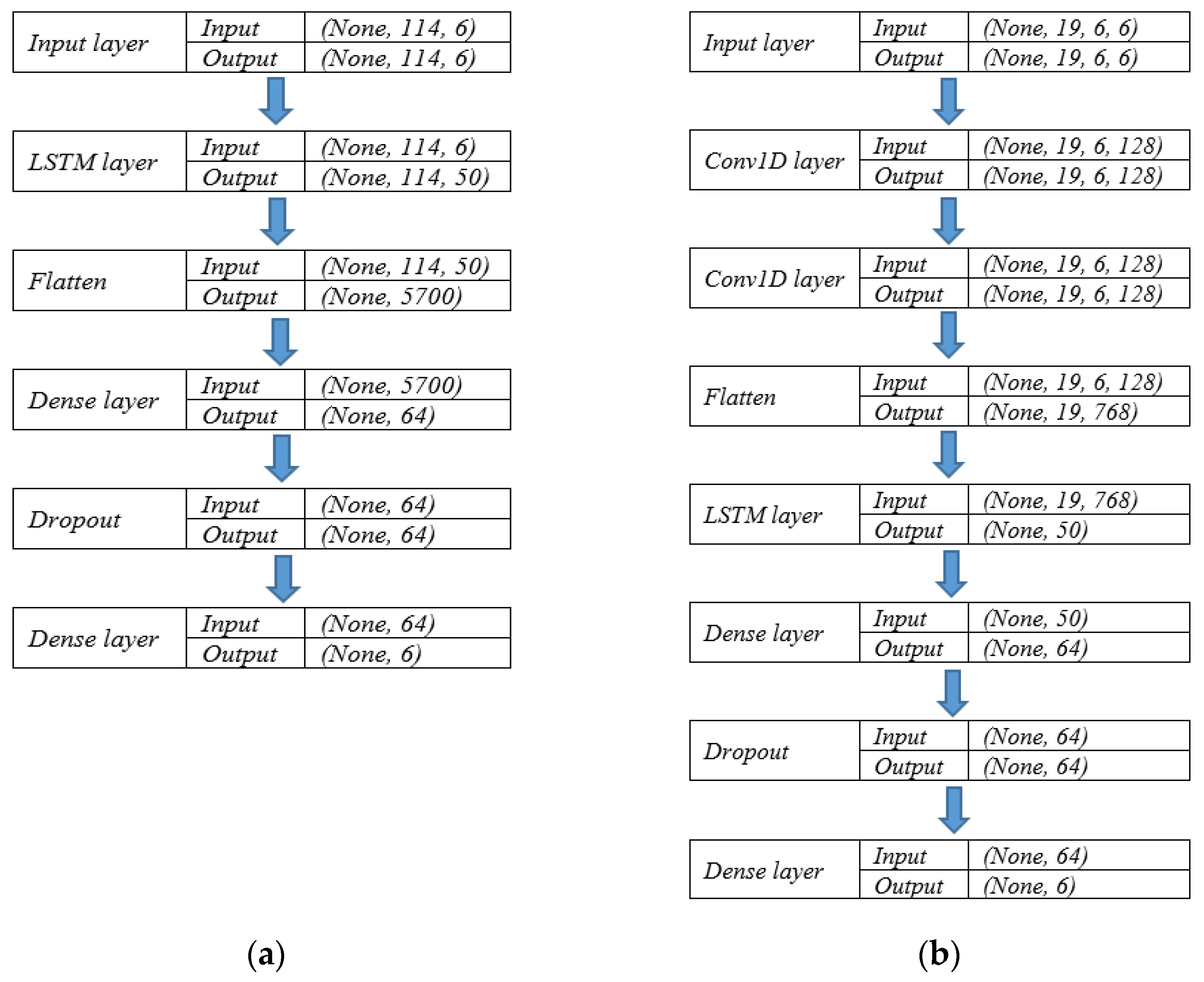
3.3. Deep Learning Models
4. Case Study
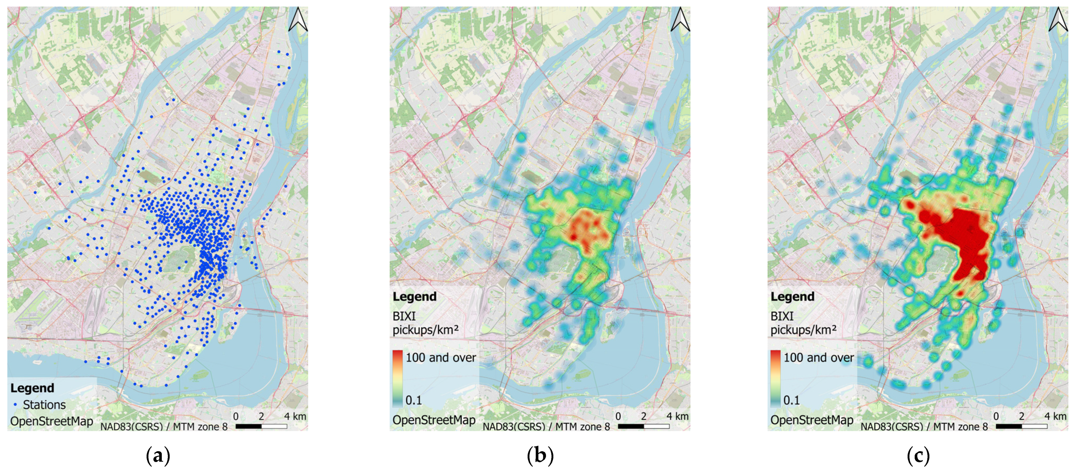
5. Community Structure in BIXI Network
6. Data Preparation for Modeling
6.1. Selected Variables
6.2. Model Specification
6.3. Model Implementation and Performance Metrics
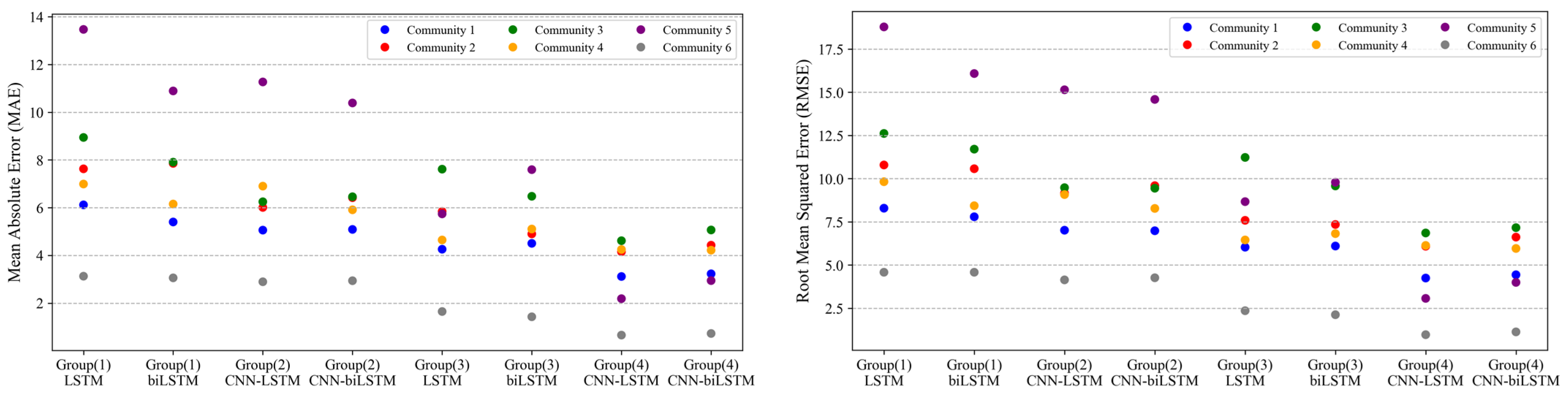
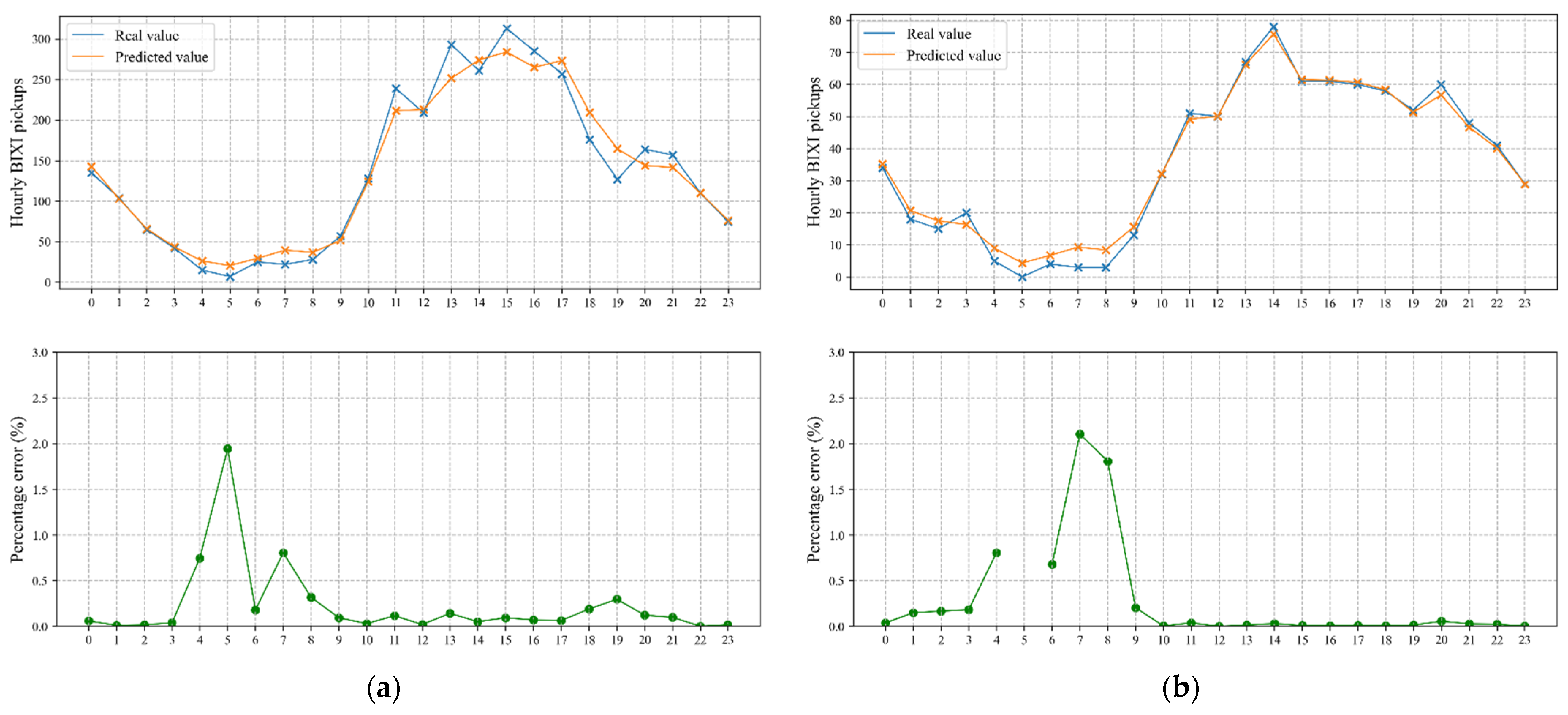
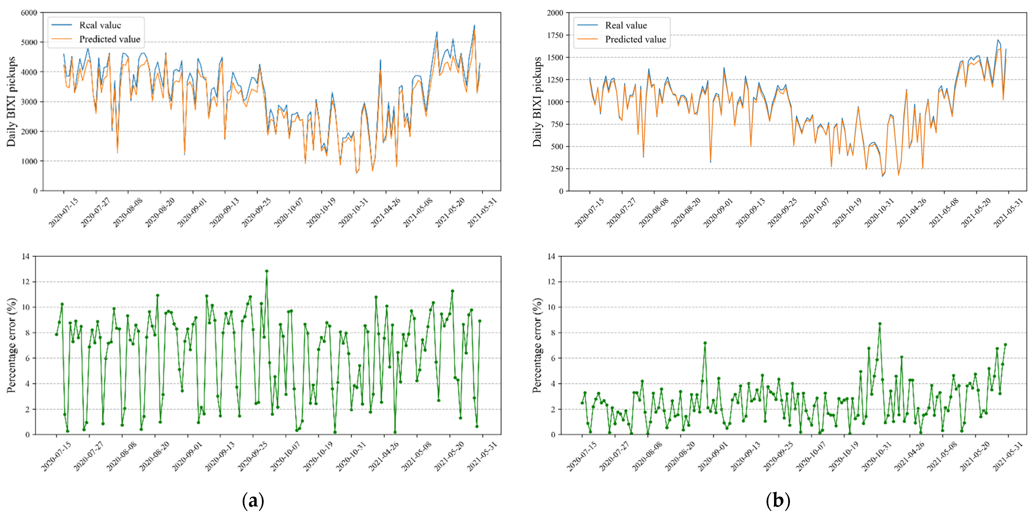
7. Prediction Results

| Model | MAE | RMSE | Epoch | Time 1 | ||
|---|---|---|---|---|---|---|
| Train | Test | Train | Test | |||
| • LSTM | 9.04 | 7.59 | 15.08 | 11.95 | 26 | 2 s |
| • biLSTM | 8.98 | 7.24 | 14.98 | 11.38 | 32 | 3 s |
| • CNN-LSTM | 6.09 | 5.93 | 8.95 | 9.11 | 21 | 1 s |
| • CNN-biLSTM | 6.04 | 5.93 | 9.02 | 9.32 | 27 | 2 s |
| • LSTM | 7.54 | 5.14 | 14.00 | 8.09 | 29 | 2 s |
| • biLSTM | 6.57 | 4.48 | 11.56 | 6.86 | 24 | 3 s |
| • CNN-LSTM | 3.17 | 3.00 | 4.92 | 4.77 | 57 | 2 s |
| • CNN-biLSTM | 3.25 | 3.09 | 5.03 | 4.88 | 57 | 3 s |
| Group (5): | ||||||
| • ARIMA | 8.05 | 50.95 | 12.41 | 61.17 | - | 762 s |
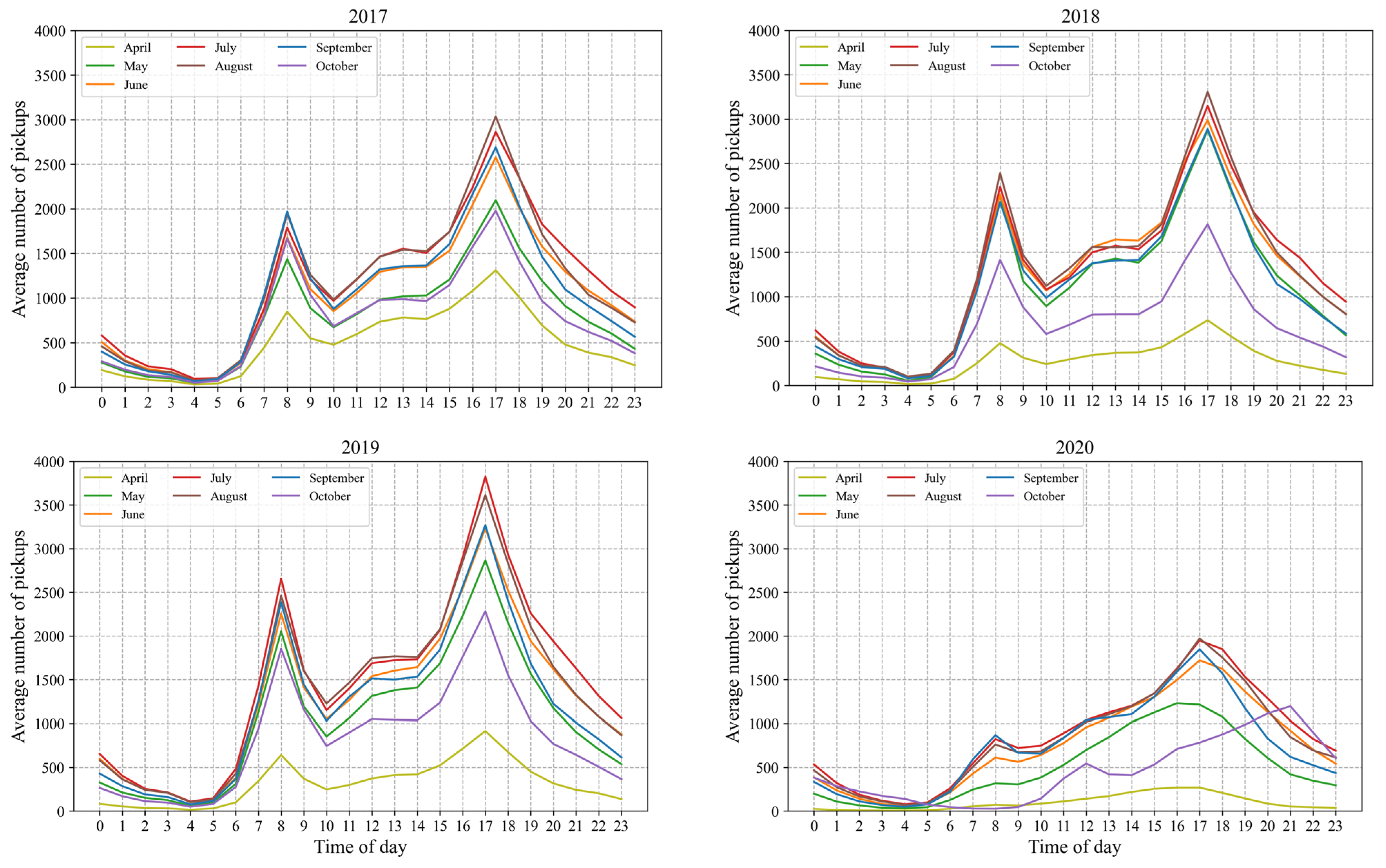
- BIXI demand has certain periodicity, and after a detailed analysis, the data clearly have hourly and daily time series periodicity. Therefore, it is essential to choose the last 24 h (i.e., 96 time steps) historical data as the input for forecasting the BIXI pickups of the next 15 min. Comparing Table 1 and Table 2 supports this statement for almost all candidate models as the selected time step provides a better prediction performance on test data;
- There are many features associated with BIXI pickup demand which may influence the accuracy and efficiency of the short-term prediction. Results show that the accuracies of deep learning models integrating the extra inputs i.e., demand related engineered features, weather conditions, and temporal variables are higher than those of univariate models for short-term prediction of the bike-sharing pickups. Therefore, it is of importance to incorporate the extra features;
- This study proposed a hybrid CNN-LSTM model to forecast bike pickup demands in different clusters of BIXI stations simultaneously, in which CNN is employed to extract related features from input data, and then LSTM is adopted to support sequence predictions. The results indicate a prominent efficiency of the proposed architecture in terms of prediction accuracy but with a longer training time.
8. Discussion and Conclusions
Author Contributions
Funding
Institutional Review Board Statement
Informed Consent Statement
Data Availability Statement
Acknowledgments
Conflicts of Interest
References
- Hatzopoulou, M.; Weichenthal, S.; Dugum, H.; Pickett, G.; Miranda-Moreno, L.; Kulka, R.; Andersen, R.; Goldberg, M. The Impact of Traffic Volume, Composition, and Road Geometry on Personal Air Pollution Exposures among Cyclists in Montreal, Canada. J. Expo. Sci. Environ. Epidemiol. 2013, 23, 46–51. [Google Scholar] [CrossRef] [PubMed]
- Shaheen, S.A.; Guzman, S.; Zhang, H. Bikesharing in Europe, the Americas, and Asia: Past, Present, and Future. Transp. Res. Rec. 2010, 2143, 159–167. [Google Scholar] [CrossRef] [Green Version]
- Qiu, L.-Y.; He, L.-Y. Bike Sharing and the Economy, the Environment, and Health-Related Externalities. Sustainability 2018, 10, 1145. [Google Scholar] [CrossRef] [Green Version]
- Murgano, E.; Caponetto, R.; Pappalardo, G.; Cafiso, S.D.; Severino, A. A Novel Acceleration Signal Processing Procedure for Cycling Safety Assessment. Sensors 2021, 21, 4183. [Google Scholar] [CrossRef] [PubMed]
- Beecham, R.; Wood, J.; Bowerman, A. Studying Commuting Behaviours Using Collaborative Visual Analytics. Comput. Environ. Urban Syst. 2014, 47, 5–15. [Google Scholar] [CrossRef]
- Guo, Y.; Zhou, J.; Wu, Y.; Li, Z. Identifying the Factors Affecting Bike-Sharing Usage and Degree of Satisfaction in Ningbo, China. PLoS ONE 2017, 12, e0185100. [Google Scholar] [CrossRef] [PubMed] [Green Version]
- Fishman, E. Bikeshare: A Review of Recent Literature. Transp. Rev. 2016, 36, 92–113. [Google Scholar] [CrossRef]
- Dastjerdi, A.M.; Kaplan, S.; de Abreu e Silva, J.; Anker Nielsen, O.; Camara Pereira, F. Use Intention of Mobility-Management Travel Apps: The Role of Users Goals, Technophile Attitude and Community Trust. Transp. Res. Part A Policy Pract. 2019, 126, 114–135. [Google Scholar] [CrossRef]
- Dastjerdi, A.M.; Kaplan, S.; e Silva, J.D.A.; Nielsen, O.A.; Pereira, F.C. Factors Driving the Adoption of Mobility-Management Travel App: A Bayesian Structural Equation Modelling Analysis. In Proceedings of the 98th Annual Meeting of the Transportation Research Board, Washington, DC, USA, 12–16 January 2019. [Google Scholar]
- Albuquerque, V.; Sales Dias, M.; Bacao, F. Machine Learning Approaches to Bike-Sharing Systems: A Systematic Literature Review. ISPRS Int. J. Geo-Inf. 2021, 10, 62. [Google Scholar] [CrossRef]
- Caulfield, B.; O’Mahony, M.; Brazil, W.; Weldon, P. Examining Usage Patterns of a Bike-Sharing Scheme in a Medium Sized City. Transp. Res. Part A Policy Pract. 2017, 100, 152–161. [Google Scholar] [CrossRef]
- Ashqar, H.I.; Elhenawy, M.; Almannaa, M.H.; Ghanem, A.; Rakha, H.A.; House, L. Modeling Bike Availability in a Bike-Sharing System Using Machine Learning. In Proceedings of the 2017 5th IEEE International Conference on Models and Technologies for Intelligent Transportation Systems (MT-ITS), Napoli, Italy, 26–28 June 2017; pp. 374–378. [Google Scholar]
- Reynaud, F.; Faghih-Imani, A.; Eluru, N. Modelling Bicycle Availability in Bicycle Sharing Systems: A Case Study from Montreal. Sustain. Cities Soc. 2018, 43, 32–40. [Google Scholar] [CrossRef]
- Sohrabi, S.; Paleti, R.; Balan, L.; Cetin, M. Real-Time Prediction of Public Bike Sharing System Demand Using Generalized Extreme Value Count Model. Transp. Res. Part A Policy Pract. 2020, 133, 325–336. [Google Scholar] [CrossRef]
- Sathishkumar, V.E.; Park, J.; Cho, Y. Using Data Mining Techniques for Bike Sharing Demand Prediction in Metropolitan City. Comput. Commun. 2020, 153, 353–366. [Google Scholar] [CrossRef]
- Pan, Y.; Zheng, R.C.; Zhang, J.; Yao, X. Predicting Bike Sharing Demand Using Recurrent Neural Networks. Procedia Comput. Sci. 2019, 147, 562–566. [Google Scholar] [CrossRef]
- Liu, X.; Gherbi, A.; Li, W.; Cheriet, M. Multi Features and Multi-Time Steps LSTM Based Methodology for Bike Sharing Availability Prediction. Procedia Comput. Sci. 2019, 155, 394–401. [Google Scholar] [CrossRef]
- Wang, B.; Kim, I. Short-Term Prediction for Bike-Sharing Service Using Machine Learning. Transp. Res. Procedia 2018, 34, 171–178. [Google Scholar] [CrossRef]
- Boonjubut, K.; Hasegawa, H. Multivariate Time Series Analysis Using Recurrent Neural Network to Predict Bike-Sharing Demand. In Smart Transportation Systems 2020, Proceedings of the 3rd KES-STS International Symposium, Virtual Conference, 17–19 June 2020; Qu, X., Zhen, L., Howlett, R.J., Jain, L.C., Eds.; Springer: Singapore, 2020; pp. 69–77. [Google Scholar]
- Li, D.; Lin, C.; Gao, W.; Meng, Z.; Song, Q. Short-Term Rental Forecast of Urban Public Bicycle Based on the HOSVD-LSTM Model in Smart City. Sensors 2020, 20, 3072. [Google Scholar] [CrossRef]
- Ai, Y.; Li, Z.; Gan, M.; Zhang, Y.; Yu, D.; Chen, W.; Ju, Y. A Deep Learning Approach on Short-Term Spatiotemporal Distribution Forecasting of Dockless Bike-Sharing System. Neural Comput. Appl. 2019, 31, 1665–1677. [Google Scholar] [CrossRef]
- Zhao, S.; Lin, S.; Xu, J. Time Series Traffic Prediction via Hybrid Neural Networks. In Proceedings of the 2019 IEEE Intelligent Transportation Systems Conference (ITSC), Auckland, New Zealand, 27–30 October 2019; pp. 1671–1676. [Google Scholar]
- Kouassi, K.H.; Moodley, D. An Analysis of Deep Neural Networks for Predicting Trends in Time Series Data. In Artificial Intelligence Research, Proceedings of the First Southern African Conference for AI Research, SACAIR 2020, Muldersdrift, South Africa, 22–26 February 2021; Springer: Berlin/Heidelberg, Germany, 2020; pp. 119–140. [Google Scholar]
- Lin, T.; Guo, T.; Aberer, K. Hybrid Neural Networks for Learning the Trend in Time Series. In Proceedings of the Twenty-Sixth International Joint Conference on Artificial Intelligence, Melbourne, Australia, 19–25 August 2017; International Joint Conferences on Artificial Intelligence Organization: Melbourne, Australia, 2017; pp. 2273–2279. [Google Scholar]
- Lin, L.; He, Z.; Peeta, S. Predicting Station-Level Hourly Demand in a Large-Scale Bike-Sharing Network: A Graph Convolutional Neural Network Approach. Transp. Res. Part C Emerg. Technol. 2018, 97, 258–276. [Google Scholar] [CrossRef] [Green Version]
- Ke, J.; Zheng, H.; Yang, H.; Chen, X. (Michael) Short-Term Forecasting of Passenger Demand under on-Demand Ride Services: A Spatio-Temporal Deep Learning Approach. Transp. Res. Part C Emerg. Technol. 2017, 85, 591–608. [Google Scholar] [CrossRef] [Green Version]
- Faghih-Imani, A.; Eluru, N. Incorporating the Impact of Spatio-Temporal Interactions on Bicycle Sharing System Demand: A Case Study of New York CitiBike System. J. Transp. Geogr. 2016, 54, 218–227. [Google Scholar] [CrossRef]
- Faghih-Imani, A.; Eluru, N.; El-Geneidy, A.M.; Rabbat, M.; Haq, U. How Land-Use and Urban Form Impact Bicycle Flows: Evidence from the Bicycle-Sharing System (BIXI) in Montreal. J. Transp. Geogr. 2014, 41, 306–314. [Google Scholar] [CrossRef]
- Yang, Z.; Hu, J.; Shu, Y.; Cheng, P.; Chen, J.; Moscibroda, T. Mobility Modeling and Prediction in Bike-Sharing Systems. In Proceedings of the 14th Annual International Conference on Mobile Systems, Applications, and Services, Singapore, 26–30 June 2016; Association for Computing Machinery: New York, NY, USA, 2016; pp. 165–178. [Google Scholar]
- Bao, J.; Shi, X.; Zhang, H. Spatial Analysis of Bikeshare Ridership With Smart Card and POI Data Using Geographically Weighted Regression Method. IEEE Access 2018, 6, 76049–76059. [Google Scholar] [CrossRef]
- Wang, K.; Akar, G.; Chen, Y.-J. Bike Sharing Differences among Millennials, Gen Xers, and Baby Boomers: Lessons Learnt from New York City’s Bike Share. Transp. Res. Part A Policy Pract. 2018, 116, 1–14. [Google Scholar] [CrossRef]
- Scott, D.M.; Ciuro, C. What Factors Influence Bike Share Ridership? An Investigation of Hamilton, Ontario’s Bike Share Hubs. Travel Behav. Soc. 2019, 16, 50–58. [Google Scholar] [CrossRef]
- Yang, Y.; Heppenstall, A.; Turner, A.; Comber, A. Using Graph Structural Information about Flows to Enhance Short-Term Demand Prediction in Bike-Sharing Systems. Comput. Environ. Urban Syst. 2020, 83, 101521. [Google Scholar] [CrossRef]
- Li, Y.; Zheng, Y.; Zhang, H.; Chen, L. Traffic Prediction in a Bike-Sharing System. In Proceedings of the 23rd SIGSPATIAL International Conference on Advances in Geographic Information Systems, Seattle, WA, USA, 3–6 November 2015; Association for Computing Machinery: New York, NY, USA, 2015; pp. 1–10. [Google Scholar]
- Zhou, Y.; Li, Y.; Zhu, Q.; Chen, F.; Shao, J.; Luo, Y.; Zhang, Y.; Zhang, P.; Yang, W. A Reliable Traffic Prediction Approach for Bike-Sharing System by Exploiting Rich Information with Temporal Link Prediction Strategy. Trans. GIS 2019, 23, 1125–1151. [Google Scholar] [CrossRef]
- Cao, Y.; Shen, D. Contribution of Shared Bikes to Carbon Dioxide Emission Reduction and the Economy in Beijing. Sustain. Cities Soc. 2019, 51, 101749. [Google Scholar] [CrossRef]
- Yang, Y.; Heppenstall, A.; Turner, A.; Comber, A. A Spatiotemporal and Graph-Based Analysis of Dockless Bike Sharing Patterns to Understand Urban Flows over the Last Mile. Comput. Environ. Urban Syst. 2019, 77, 101361. [Google Scholar] [CrossRef]
- Pase, F.; Chiariotti, F.; Zanella, A.; Zorzi, M. Bike Sharing and Urban Mobility in a Post-Pandemic World. IEEE Access 2020, 8, 187291–187306. [Google Scholar] [CrossRef]
- Shang, W.-L.; Chen, J.; Bi, H.; Sui, Y.; Chen, Y.; Yu, H. Impacts of COVID-19 Pandemic on User Behaviors and Environmental Benefits of Bike Sharing: A Big-Data Analysis. Appl. Energy 2021, 285, 116429. [Google Scholar] [CrossRef] [PubMed]
- Padmanabhan, V.; Penmetsa, P.; Li, X.; Dhondia, F.; Dhondia, S.; Parrish, A. COVID-19 Effects on Shared-Biking in New York, Boston, and Chicago. Transp. Res. Interdiscip. Perspect. 2021, 9, 100282. [Google Scholar] [CrossRef]
- Teixeira, J.F.; Lopes, M. The Link between Bike Sharing and Subway Use during the COVID-19 Pandemic: The Case-Study of New York’s Citi Bike. Transp. Res. Interdiscip. Perspect. 2020, 6, 100166. [Google Scholar] [CrossRef] [PubMed]
- Hu, S.; Xiong, C.; Liu, Z.; Zhang, L. Examining Spatiotemporal Changing Patterns of Bike-Sharing Usage during COVID-19 Pandemic. J. Transp. Geogr. 2021, 91, 102997. [Google Scholar] [CrossRef] [PubMed]
- Wei, W.; Yan, X. A Novel Deep Recurrent Neural Network for Short-Term Travel Demand Forecasting under on-Demand Ride Services. IOP Conf. Ser. Mater. Sci. Eng. 2019, 688, 033022. [Google Scholar] [CrossRef]
- Blondel, V.D.; Guillaume, J.-L.; Lambiotte, R.; Lefebvre, E. Fast Unfolding of Communities in Large Networks. J. Stat. Mech. 2008, 2008, P10008. [Google Scholar] [CrossRef] [Green Version]
- Lancichinetti, A.; Fortunato, S. Community Detection Algorithms: A Comparative Analysis. Phys. Rev. E 2009, 80, 056117. [Google Scholar] [CrossRef] [Green Version]
- Hochreiter, S.; Schmidhuber, J. Long Short-Term Memory. Neural Comput. 1997, 9, 1735–1780. [Google Scholar] [CrossRef]
- Lecun, Y.; Bottou, L.; Bengio, Y.; Haffner, P. Gradient-Based Learning Applied to Document Recognition. Proc. IEEE 1998, 86, 2278–2324. [Google Scholar] [CrossRef] [Green Version]
- Velastegui, R.; Zhinin-Vera, L.; Pilliza, G.E.; Chang, O. Time Series Prediction by Using Convolutional Neural Networks. In Proceedings of the Future Technologies Conference (FTC) 2020, Vancouver, BC, Canada, 5–6 November 2020; Arai, K., Kapoor, S., Bhatia, R., Eds.; Springer International Publishing: Cham, Switzerland, 2021; Volume 1, pp. 499–511. [Google Scholar]
- Gunduz, H.; Yaslan, Y.; Cataltepe, Z. Intraday Prediction of Borsa Istanbul Using Convolutional Neural Networks and Feature Correlations. Knowl.-Based Syst. 2017, 137, 138–148. [Google Scholar] [CrossRef]
- Cao, M.; Li, V.O.K.; Chan, V.W.S. A CNN-LSTM Model for Traffic Speed Prediction. In Proceedings of the 2020 IEEE 91st Vehicular Technology Conference (VTC2020-Spring), Antwerp, Belgium, 25–28 May 2020; pp. 1–5. [Google Scholar]
- Shu, P.; Sun, Y.; Zhao, Y.; Xu, G. Spatial-Temporal Taxi Demand Prediction Using LSTM-CNN. In Proceedings of the 2020 IEEE 16th International Conference on Automation Science and Engineering (CASE), Hong Kong, China, 20–21 August 2020; pp. 1226–1230. [Google Scholar]
- Boulila, W.; Ghandorh, H.; Khan, M.A.; Ahmed, F.; Ahmad, J. A Novel CNN-LSTM-Based Approach to Predict Urban Expansion. Ecol. Inform. 2021, 64, 101325. [Google Scholar] [CrossRef]
- Bucsky, P. Modal Share Changes Due to COVID-19: The Case of Budapest. Transp. Res. Interdiscip. Perspect. 2020, 8, 100141. [Google Scholar] [CrossRef]
- Chai, X.; Guo, X.; Xiao, J.; Jiang, J. Analysis of Spatial-Temporal Behavior Pattern of the Share Bike Usage during COVID-19 Pandemic in Beijing. arXiv 2021, arXiv:2004.12340. [Google Scholar]
- Nikiforiadis, A.; Ayfantopoulou, G.; Stamelou, A. Assessing the Impact of COVID-19 on Bike-Sharing Usage: The Case of Thessaloniki, Greece. Sustainability 2020, 12, 8215. [Google Scholar] [CrossRef]
- Du, Y.; Deng, F.; Liao, F. A Model Framework for Discovering the Spatio-Temporal Usage Patterns of Public Free-Floating Bike-Sharing System. Transp. Res. Part C Emerg. Technol. 2019, 103, 39–55. [Google Scholar] [CrossRef]
- Li, A.; Axhausen, K.W. Comparison of Short-Term Traffic Demand Prediction Methods for Transport Services. Arb. Verk.-Und Raumplan. 2019, 1447. [Google Scholar] [CrossRef]


| Model | 24 (6 h) | 48 (12 h) | 192 (48 h) | 672 (1 Week) | ||||
|---|---|---|---|---|---|---|---|---|
| MAE | RMSE | MAE | RMSE | MAE | RMSE | MAE | RMSE | |
| Group (1): | ||||||||
| • LSTM | 7.47 | 11.18 | 8.35 | 12.46 | 7.04 | 10.91 | 15.62 | 20.42 |
| • biLSTM | 7.47 | 11.08 | 7.56 | 11.62 | 7.14 | 10.83 | 20.74 | 27.41 |
| Group (2): | ||||||||
| • CNN-LSTM | 5.74 | 8.97 | 5.92 | 9.31 | 6.86 | 9.89 | 6.27 | 9.54 |
| • CNN-biLSTM | 5.98 | 9.47 | 6.23 | 9.37 | 6.81 | 10.11 | 5.81 | 9.01 |
| Group (3): | ||||||||
| • LSTM | 5.51 | 9.29 | 6.46 | 9.99 | 5.42 | 8.97 | 6.62 | 9.97 |
| • biLSTM | 4.52 | 7.16 | 5.43 | 7.93 | 10.32 | 14.42 | 21.41 | 28.11 |
| Group (4): | ||||||||
| • CNN-LSTM | 3.28 | 5.02 | 3.24 | 5.08 | 3.12 | 4.81 | 3.08 | 4.74 |
| • CNN-biLSTM | 3.34 | 5.09 | 3.25 | 5.03 | 3.35 | 5.12 | 3.53 | 5.16 |
| Group (5): | ||||||||
| • ARIMA | 50.94 | 61.16 | 50.94 | 61.16 | 50.95 | 61.17 | 51.00 | 61.22 |
Publisher’s Note: MDPI stays neutral with regard to jurisdictional claims in published maps and institutional affiliations. |
© 2022 by the authors. Licensee MDPI, Basel, Switzerland. This article is an open access article distributed under the terms and conditions of the Creative Commons Attribution (CC BY) license (https://creativecommons.org/licenses/by/4.0/).
Share and Cite
Mehdizadeh Dastjerdi, A.; Morency, C. Bike-Sharing Demand Prediction at Community Level under COVID-19 Using Deep Learning. Sensors 2022, 22, 1060. https://doi.org/10.3390/s22031060
Mehdizadeh Dastjerdi A, Morency C. Bike-Sharing Demand Prediction at Community Level under COVID-19 Using Deep Learning. Sensors. 2022; 22(3):1060. https://doi.org/10.3390/s22031060
Chicago/Turabian StyleMehdizadeh Dastjerdi, Aliasghar, and Catherine Morency. 2022. "Bike-Sharing Demand Prediction at Community Level under COVID-19 Using Deep Learning" Sensors 22, no. 3: 1060. https://doi.org/10.3390/s22031060
APA StyleMehdizadeh Dastjerdi, A., & Morency, C. (2022). Bike-Sharing Demand Prediction at Community Level under COVID-19 Using Deep Learning. Sensors, 22(3), 1060. https://doi.org/10.3390/s22031060