
An Adaptive Refinement Scheme for Depth Estimation Networks


Abstract
1. Introduction
- A novel double-stage adaptive refinement scheme for monocular depth estimation networks. The proposed scheme needs neither offline data gathering nor offline training, because it uses available pre-trained weights.
- Introduction of functional adaptation schemes in the field of depth generation, for the first time. Using the proposed adaptive scheme, pre-trained networks can be straightforwardly used for unseen datasets through adjusting the shape of activation functions of an intermediate layer.
- A model-agnostic scheme which can be plugged into any baseline. In this paper, we selected Monodepth2 [23] as one of the most widely used baselines for depth estimation.
2. Related Work
2.1. Unsupervised Depth Estimation Methods
2.2. Supervised Depth Estimation Methods
2.3. Functionally Adaptive Neural Networks
3. Theoretical Background
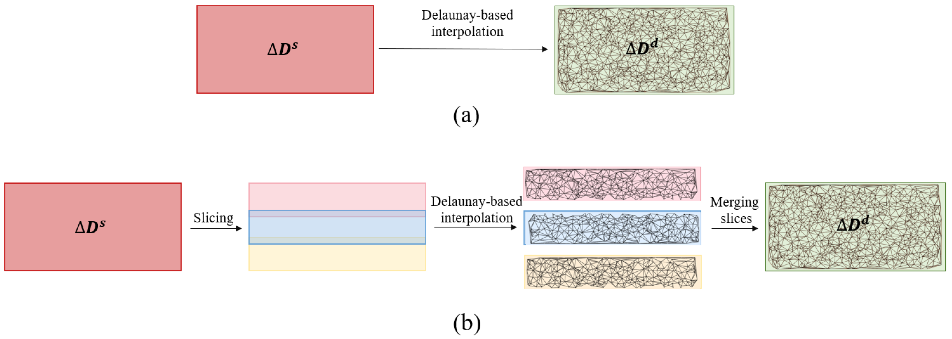
3.1. Delaunay-Based Interpolation
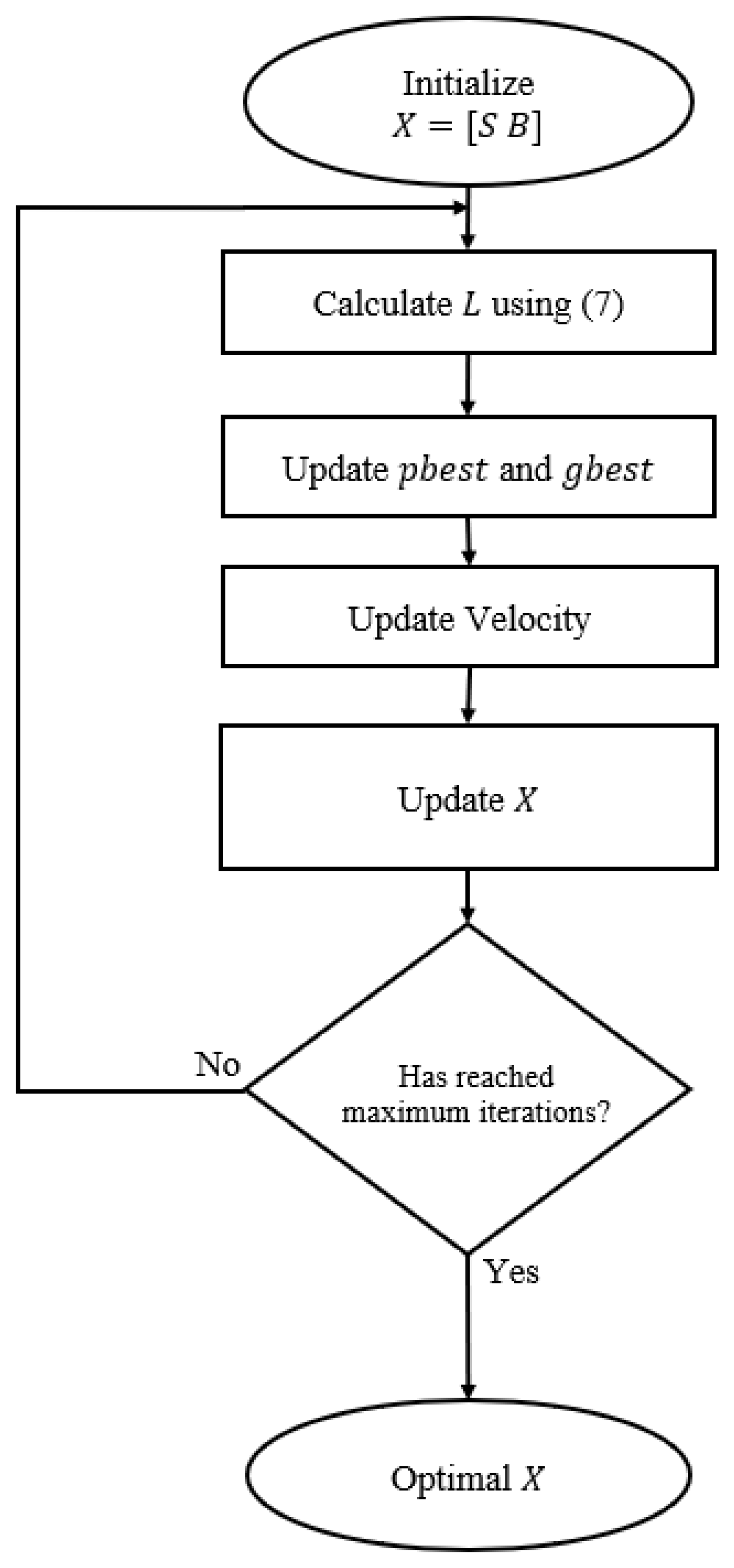
3.2. PSO
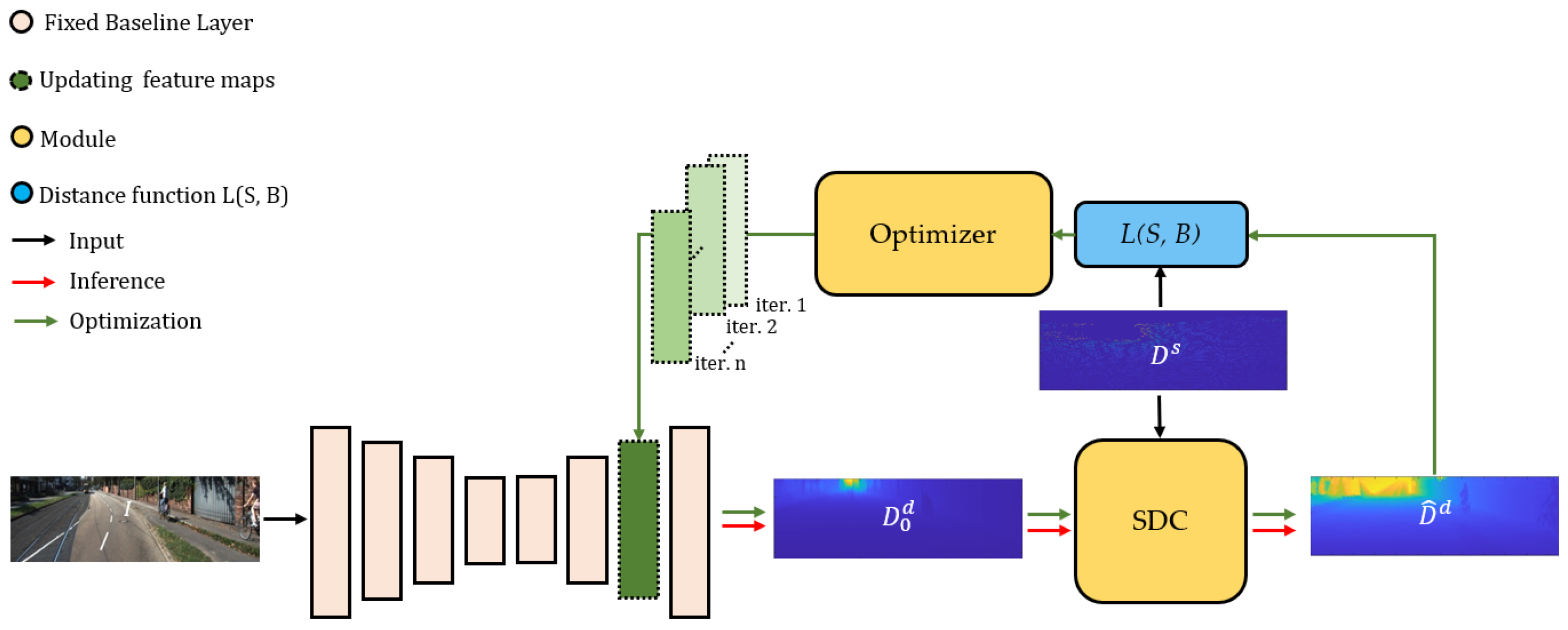
4. Proposed Method
4.1. Baseline
4.2. Correction
4.3. Activation Optimization
4.3.1. Overall Scheme
4.3.2. Optimizer
5. Experiments
5.1. Datasets
5.1.1. KITTI
5.1.2. NYUv2
5.2. Assessment Criteria
5.3. Network Architecture
5.4. Implementation Details
5.5. Ablation Studies
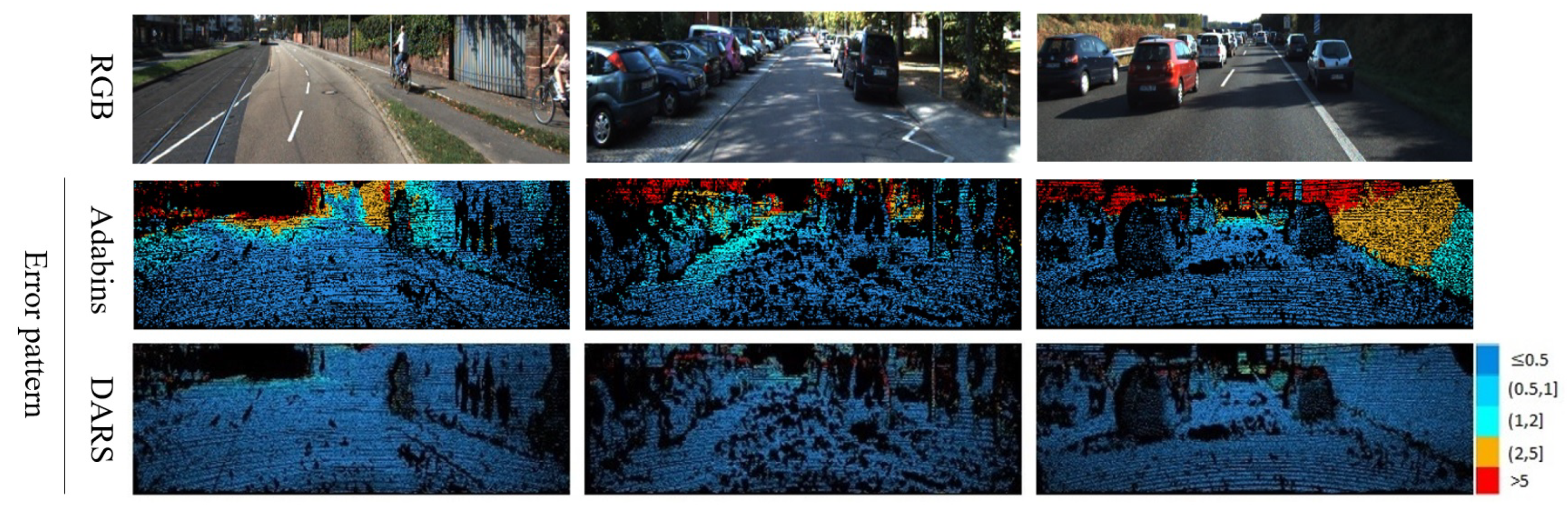
5.6. Comparison with SOTA
6. Conclusions
Author Contributions
Funding
Institutional Review Board Statement
Informed Consent Statement
Data Availability Statement
Conflicts of Interest
References
- Yousif, K.; Taguchi, Y.; Ramalingam, S. MonoRGBD-SLAM: Simultaneous localization and mapping using both monocular and RGBD cameras. In Proceedings of the 2017 IEEE International Conference on Robotics and Automation (ICRA), Singapore, 29 May–3 June 2017; IEEE: Piscataway Township, NJ, USA, 2017; pp. 4495–4502. [Google Scholar]
- Li, R.; Wang, S.; Long, Z.; Gu, D. Undeepvo: Monocular visual odometry through unsupervised deep learning. In Proceedings of the 2018 IEEE international conference on robotics and automation (ICRA), Brisbane, Australia, 21–25 May 2018; IEEE: Piscataway Township, NJ, USA, 2018; pp. 7286–7291. [Google Scholar]
- Dimas, G.; Gatoula, P.; Iakovidis, D.K. MonoSOD: Monocular Salient Object Detection based on Predicted Depth. In Proceedings of the 2021 IEEE International Conference on Robotics and Automation (ICRA), Xi’an, China, 30 May–5 June 2021; IEEE: Piscataway Township, NJ, USA, 2021; pp. 4377–4383. [Google Scholar]
- Hu, M.; Wang, S.; Li, B.; Ning, S.; Fan, L.; Gong, X. PENet: Towards Precise and Efficient Image Guided Depth Completion. arXiv 2021, arXiv:2103.00783. [Google Scholar]
- Park, J.; Joo, K.; Hu, Z.; Liu, C.K.; So Kweon, I. Non-local spatial propagation network for depth completion. In Proceedings of the Computer Vision–ECCV 2020: 16th European Conference, Glasgow, UK, 23–28 August 2020; Springer: Berlin/Heidelberg, Germany, 2020; pp. 120–136. [Google Scholar]
- Gurram, A.; Tuna, A.F.; Shen, F.; Urfalioglu, O.; López, A.M. Monocular Depth Estimation through Virtual-world Supervision and Real-world SfM Self-Supervision. arXiv 2021, arXiv:2103.12209. [Google Scholar] [CrossRef]
- Hirose, N.; Koide, S.; Kawano, K.; Kondo, R. Plg-in: Pluggable geometric consistency loss with wasserstein distance in monocular depth estimation. In Proceedings of the 2021 IEEE International Conference on Robotics and Automation (ICRA), Xi’an, China, 30 May–5 June 2021; IEEE: Piscataway Township, NJ, USA, 2021; pp. 12868–12874. [Google Scholar]
- Liu, J.; Li, Q.; Cao, R.; Tang, W.; Qiu, G. MiniNet: An extremely lightweight convolutional neural network for real-time unsupervised monocular depth estimation. ISPRS J. Photogramm. Remote Sens. 2020, 166, 255–267. [Google Scholar] [CrossRef]
- Hwang, S.J.; Park, S.J.; Kim, G.M.; Baek, J.H. Unsupervised Monocular Depth Estimation for Colonoscope System Using Feedback Network. Sensors 2021, 21, 2691. [Google Scholar] [CrossRef]
- Wang, Y.; Zhu, H. Monocular Depth Estimation: Lightweight Convolutional and Matrix Capsule Feature-Fusion Network. Sensors 2022, 22, 6344. [Google Scholar] [CrossRef]
- Cheng, X.; Wang, P.; Guan, C.; Yang, R. Cspn++: Learning context and resource aware convolutional spatial propagation networks for depth completion. In Proceedings of the AAAI Conference on Artificial Intelligence, New York, NY, USA, 7–12 February 2020; Volume 34, pp. 10615–10622. [Google Scholar]
- Kuznietsov, Y.; Stuckler, J.; Leibe, B. Semi-supervised deep learning for monocular depth map prediction. In Proceedings of the IEEE Conference on Computer Vision and Pattern Recognition, Honolulu, HI, USA, 21–26 July 2017; pp. 6647–6655. [Google Scholar]
- Huang, Y.K.; Liu, Y.C.; Wu, T.H.; Su, H.T.; Chang, Y.C.; Tsou, T.L.; Wang, Y.A.; Hsu, W.H. S3: Learnable Sparse Signal Superdensity for Guided Depth Estimation. In Proceedings of the IEEE/CVF Conference on Computer Vision and Pattern Recognition, Nashville, TN, USA, 20–25 June 2021; pp. 16706–16716. [Google Scholar]
- Bhat, S.F.; Alhashim, I.; Wonka, P. Adabins: Depth estimation using adaptive bins. In Proceedings of the IEEE/CVF Conference on Computer Vision and Pattern Recognition, Nashville, TN, USA, 20–25 June 2021; pp. 4009–4018. [Google Scholar]
- Lee, J.H.; Han, M.K.; Ko, D.W.; Suh, I.H. From big to small: Multi-scale local planar guidance for monocular depth estimation. arXiv 2019, arXiv:1907.10326. [Google Scholar]
- Lee, S.; Lee, J.; Kim, B.; Yi, E.; Kim, J. Patch-Wise Attention Network for Monocular Depth Estimation. In Proceedings of the AAAI Conference on Artificial Intelligence, Virtual, 2–9 February 2021; Volume 35, pp. 1873–1881. [Google Scholar]
- Liu, Y.; Yixuan, Y.; Liu, M. Ground-aware monocular 3d object detection for autonomous driving. IEEE Robot. Autom. Lett. 2021, 6, 919–926. [Google Scholar] [CrossRef]
- Jang, W.D.; Kim, C.S. Interactive Image Segmentation via Backpropagating Refinement Scheme. In Proceedings of the IEEE/CVF Conference on Computer Vision and Pattern Recognition (CVPR), Long Beach, CA, USA, 15–20 June 2019. [Google Scholar]
- Sofiiuk, K.; Petrov, I.; Barinova, O.; Konushin, A. f-brs: Rethinking backpropagating refinement for interactive segmentation. In Proceedings of the IEEE/CVF Conference on Computer Vision and Pattern Recognition, Seattle, WA, USA, 14–19 June 2020; pp. 8623–8632. [Google Scholar]
- Lau, M.M.; Lim, K.H. Review of adaptive activation function in deep neural network. In Proceedings of the 2018 IEEE-EMBS Conference on Biomedical Engineering and Sciences (IECBES), Sarawak, Malaysia, 3–6 December 2018; IEEE: Piscataway Township, NJ, USA, 2018; pp. 686–690. [Google Scholar]
- Huang, X.; Belongie, S. Arbitrary style transfer in real-time with adaptive instance normalization. In Proceedings of the IEEE International Conference on Computer Vision, Venice, Italy, 22–29 October 2017; pp. 1501–1510. [Google Scholar]
- Kennedy, J.; Eberhart, R. Particle swarm optimization. In Proceedings of the ICNN’95-International Conference on Neural Networks, Perth, WA, Australia, 27 November–1 December 1995; IEEE: Piscataway Township, NJ, USA, 1995; Volume 4, pp. 1942–1948. [Google Scholar]
- Godard, C.; Mac Aodha, O.; Firman, M.; Brostow, G.J. Digging into self-supervised monocular depth estimation. In Proceedings of the IEEE/CVF International Conference on Computer Vision, Montreal, BC, Canada, 11–17 October 2017; pp. 3828–3838. [Google Scholar]
- Zhou, T.; Brown, M.; Snavely, N.; Lowe, D.G. Unsupervised learning of depth and ego-motion from video. In Proceedings of the IEEE Conference on Computer Vision and Pattern Recognition, Honolulu, HI, USA, 21–26 July 2017; pp. 1851–1858. [Google Scholar]
- Ye, X.; Ji, X.; Sun, B.; Chen, S.; Wang, Z.; Li, H. DRM-SLAM: Towards dense reconstruction of monocular SLAM with scene depth fusion. Neurocomputing 2020, 396, 76–91. [Google Scholar] [CrossRef]
- Godard, C.; Mac Aodha, O.; Brostow, G.J. Unsupervised monocular depth estimation with left-right consistency. In Proceedings of the IEEE Conference on Computer Vision and Pattern Recognition, Honolulu, HI, USA, 21–26 July 2017; pp. 270–279. [Google Scholar]
- Bian, J.; Li, Z.; Wang, N.; Zhan, H.; Shen, C.; Cheng, M.M.; Reid, I. Unsupervised scale-consistent depth and ego-motion learning from monocular video. Adv. Neural Inf. Process. Syst. 2019, 32, 35–45. [Google Scholar]
- Yin, Z.; Shi, J. Geonet: Unsupervised learning of dense depth, optical flow and camera pose. In Proceedings of the IEEE Conference on Computer Vision and Pattern Recognition, Salt Lake City, UT, USA, 18–20 June 2018; pp. 1983–1992. [Google Scholar]
- Cai, H.; Matai, J.; Borse, S.; Zhang, Y.; Ansari, A.; Porikli, F. X-Distill: Improving Self-Supervised Monocular Depth via Cross-Task Distillation. arXiv 2021, arXiv:2110.12516. [Google Scholar]
- Feng, T.; Gu, D. Sganvo: Unsupervised deep visual odometry and depth estimation with stacked generative adversarial networks. IEEE Robot. Autom. Lett. 2019, 4, 4431–4437. [Google Scholar] [CrossRef]
- Ji, P.; Li, R.; Bhanu, B.; Xu, Y. Monoindoor: Towards good practice of self-supervised monocular depth estimation for indoor environments. In Proceedings of the IEEE/CVF International Conference on Computer Vision, Montreal, BC, Canada, 11–17 October 2021; pp. 12787–12796. [Google Scholar]
- Fei, X.; Wong, A.; Soatto, S. Geo-supervised visual depth prediction. IEEE Robot. Autom. Lett. 2019, 4, 1661–1668. [Google Scholar] [CrossRef]
- dos Santos Rosa, N.; Guizilini, V.; Grassi, V. Sparse-to-continuous: Enhancing monocular depth estimation using occupancy maps. In Proceedings of the 2019 19th International Conference on Advanced Robotics (ICAR), Belo Horizonte, Brazil, 2–6 December 2019; IEEE: Piscataway Township, NJ, USA, 2019; pp. 793–800. [Google Scholar]
- Ma, F.; Cavalheiro, G.V.; Karaman, S. Self-supervised sparse-to-dense: Self-supervised depth completion from lidar and monocular camera. In Proceedings of the 2019 International Conference on Robotics and Automation (ICRA), Montreal, QC, Canada, 20–24 May 2019; IEEE: Piscataway Township, NJ, USA, 2019; pp. 3288–3295. [Google Scholar]
- Ming, Y.; Meng, X.; Fan, C.; Yu, H. Deep learning for monocular depth estimation: A review. Neurocomputing 2021, 438, 14–33. [Google Scholar] [CrossRef]
- Palnitkar, R.M.; Cannady, J. A review of adaptive neural networks. In Proceedings of the IEEE SoutheastCon, Greensboro, NC, USA, 26–29 March 2004; IEEE: Piscataway Township, NJ, USA, 2004; pp. 38–47. [Google Scholar]
- Kontogianni, T.; Gygli, M.; Uijlings, J.; Ferrari, V. Continuous adaptation for interactive object segmentation by learning from corrections. In European Conference on Computer Vision; Springer: Cham, Switzerland, 2020; pp. 579–596. [Google Scholar]
- Gatys, L.; Ecker, A.S.; Bethge, M. Texture synthesis using convolutional neural networks. In Advances in Neural Information Processing Systems 28; Curran Associates, Inc.: Red Hook, NY, USA, 2015. [Google Scholar]
- Gatys, L.A.; Ecker, A.S.; Bethge, M. Image style transfer using convolutional neural networks. In Proceedings of the IEEE Conference on Computer Vision and Pattern Recognition, Las Vegas, NV, USA, 27–30 June 2016; pp. 2414–2423. [Google Scholar]
- Simonyan, K.; Vedaldi, A.; Zisserman, A. Deep inside convolutional networks: Visualising image classification models and saliency maps. arXiv 2013, arXiv:1312.6034. [Google Scholar]
- Zhang, J.; Bargal, S.A.; Lin, Z.; Brandt, J.; Shen, X.; Sclaroff, S. Top-down neural attention by excitation backprop. Int. J. Comput. Vis. 2018, 126, 1084–1102. [Google Scholar] [CrossRef]
- Amidror, I. Scattered data interpolation methods for electronic imaging systems: A survey. J. Electron. Imaging 2002, 11, 157–176. [Google Scholar] [CrossRef]
- Zhu, C.; Byrd, R.H.; Lu, P.; Nocedal, J. Algorithm 778: L-BFGS-B: Fortran subroutines for large-scale bound-constrained optimization. ACM Trans. Math. Softw. (TOMS) 1997, 23, 550–560. [Google Scholar] [CrossRef]
- Byrd, R.H.; Lu, P.; Nocedal, J.; Zhu, C. A limited memory algorithm for bound constrained optimization. SIAM J. Sci. Comput. 1995, 16, 1190–1208. [Google Scholar] [CrossRef]
- Geiger, A.; Lenz, P.; Stiller, C.; Urtasun, R. Vision meets robotics: The kitti dataset. Int. J. Robot. Res. 2013, 32, 1231–1237. [Google Scholar] [CrossRef]
- Silberman, N.; Hoiem, D.; Kohli, P.; Fergus, R. Indoor segmentation and support inference from rgbd images. In European Conference on Computer Vision; Springer: Berlin/Heidelberg, Germany, 2012; pp. 746–760. [Google Scholar]
- Eigen, D.; Puhrsch, C.; Fergus, R. Depth map prediction from a single image using a multi-scale deep network. arXiv 2014, arXiv:1406.2283. [Google Scholar]
- Paszke, A.; Gross, S.; Massa, F.; Lerer, A.; Bradbury, J.; Chanan, G.; Killeen, T.; Lin, Z.; Gimelshein, N.; Antiga, L.; et al. PyTorch: An Imperative Style, High-Performance Deep Learning Library. In Advances in Neural Information Processing Systems 32; Wallach, H., Larochelle, H., Beygelzimer, A., d’Alché-Buc, F., Fox, E., Garnett, R., Eds.; Curran Associates, Inc.: Red Hook, NY, USA, 2019; pp. 8024–8035. [Google Scholar]
- Luo, C.; Yang, Z.; Wang, P.; Wang, Y.; Xu, W.; Nevatia, R.; Yuille, A. Every pixel counts++: Joint learning of geometry and motion with 3d holistic understanding. IEEE Trans. Pattern Anal. Mach. Intell. 2019, 42, 2624–2641. [Google Scholar] [CrossRef] [PubMed]
- Zhang, J.; Li, W.; Gou, H.; Fang, L.; Yang, R. LEAD: LiDAR Extender for Autonomous Driving. arXiv 2021, arXiv:2102.07989. [Google Scholar]
- Lee, M.; Hwang, S.; Park, C.; Lee, S. EdgeConv with Attention Module for Monocular Depth Estimation. arXiv 2021, arXiv:2106.08615. [Google Scholar]


| Dataset | Modules | Lower Is Better | Higher Is Better | ||||||
|---|---|---|---|---|---|---|---|---|---|
| Baseline | Correction | Optimizer | AbsRel | RMSE | |||||
| KITTI | Monodepth2 | - | - | 0.090 | 3.942 | 0.137 | 0.914 | 0.983 | 0.995 |
| Monodepth2* | - | - | 0.996 | 19.324 | 5.715 | 0.000 | 0.000 | 0.000 | |
| Monodepth2* | DC | - | 0.864 | 16.888 | 3.149 | 0.183 | 0.330 | 0.447 | |
| Monodepth2* | SDC | - | 0.046 | 1.676 | 0.091 | 0.976 | 0.991 | 0.995 | |
| Monodepth2* | SDC | L-BFGS | 0.046 | 1.676 | 0.091 | 0.976 | 0.991 | 0.995 | |
| Monodepth2* | SDC | PSO | 0.024 | 1.440 | 0.071 | 0.985 | 0.993 | 0.996 | |
| NYUv2 | Monodepth2* | SDC | - | 0.018 | 0.766 | 0.747 | 0.972 | 0.974 | 0.975 |
| Monodepth2* | SDC | L-BFGS | 0.018 | 0.766 | 0.747 | 0.972 | 0.974 | 0.975 | |
| Monodepth2* | SDC | PSO | 0.017 | 0.109 | 0.044 | 0.993 | 0.996 | 0.999 | |
| Method | Lower Is Better | Higher Is Better | |||||
|---|---|---|---|---|---|---|---|
| AbsRel | SqRel | RMSE | |||||
| [49] | 0.120 | 0.789 | 4.755 | 0.177 | 0.856 | 0.961 | 0.987 |
| [28] | 0.132 | 0.994 | 5.240 | 0.193 | 0.833 | 0.953 | 0.985 |
| [26] | 0.114 | 0.898 | 4.935 | 0.206 | 0.861 | 0.949 | 0.976 |
| [23] | 0.090 | 0.545 | 3.942 | 0.137 | 0.914 | 0.983 | 0.995 |
| [50] | 0.090 | 0.424 | 3.419 | 0.133 | 0.916 | 0.984 | 0.996 |
| [51] | 0.060 | 0.231 | 2.642 | 0.094 | 0.958 | 0.994 | 0.999 |
| [14] | 0.058 | 0.190 | 2.360 | 0.088 | 0.964 | 0.995 | 0.999 |
| DARS | 0.024 | 0.137 | 1.442 | 0.071 | 0.985 | 0.993 | 0.996 |
| Method | Lower Is Better | Higher Is Better | ||||
|---|---|---|---|---|---|---|
| AbsRel | RMSE | |||||
| [47] | 0.158 | 0.641 | - | 0.769 | 0.950 | 0.988 |
| [15] | 0.110 | 0.392 | 0.047 | 0.885 | 0.978 | 0.994 |
| [51] | 0.107 | 0.373 | 0.046 | 0.893 | 0.985 | 0.997 |
| [14] | 0.103 | 0.364 | 0.044 | 0.903 | 0.984 | 0.997 |
| DARS | 0.017 | 0.109 | 0.044 | 0.993 | 0.996 | 0.999 |
Publisher’s Note: MDPI stays neutral with regard to jurisdictional claims in published maps and institutional affiliations. |
© 2022 by the authors. Licensee MDPI, Basel, Switzerland. This article is an open access article distributed under the terms and conditions of the Creative Commons Attribution (CC BY) license (https://creativecommons.org/licenses/by/4.0/).
Share and Cite
Alizadeh Naeini, A.; Sheikholeslami, M.M.; Sohn, G. An Adaptive Refinement Scheme for Depth Estimation Networks. Sensors 2022, 22, 9755. https://doi.org/10.3390/s22249755
Alizadeh Naeini A, Sheikholeslami MM, Sohn G. An Adaptive Refinement Scheme for Depth Estimation Networks. Sensors. 2022; 22(24):9755. https://doi.org/10.3390/s22249755
Chicago/Turabian StyleAlizadeh Naeini, Amin, Mohammad Moein Sheikholeslami, and Gunho Sohn. 2022. "An Adaptive Refinement Scheme for Depth Estimation Networks" Sensors 22, no. 24: 9755. https://doi.org/10.3390/s22249755
APA StyleAlizadeh Naeini, A., Sheikholeslami, M. M., & Sohn, G. (2022). An Adaptive Refinement Scheme for Depth Estimation Networks. Sensors, 22(24), 9755. https://doi.org/10.3390/s22249755