
Learning for Data Synthesis: Joint Local Salient Projection and Adversarial Network Optimization for Vehicle Re-Identification


Abstract
1. Introduction
- Incorporation of an attention mechanism to locate the perspective region and the intensity of the perspective.
- Data augmentation by increasing the difficulty rather than adding more images, without losing the original structure of a dataset.
- An innovative framework that combines an attention mechanism, geometric data augmentation, and deep learning.
- An innovative adversarial strategy that integrates the salient projection region location and the local region projection transformation.
2. Related Work
2.1. Vehicle ReID
2.2. Generative Adversarial Networks
2.3. Data Augmentation
2.4. Salient Region Locating
3. Methodology
3.1. Overall Framework
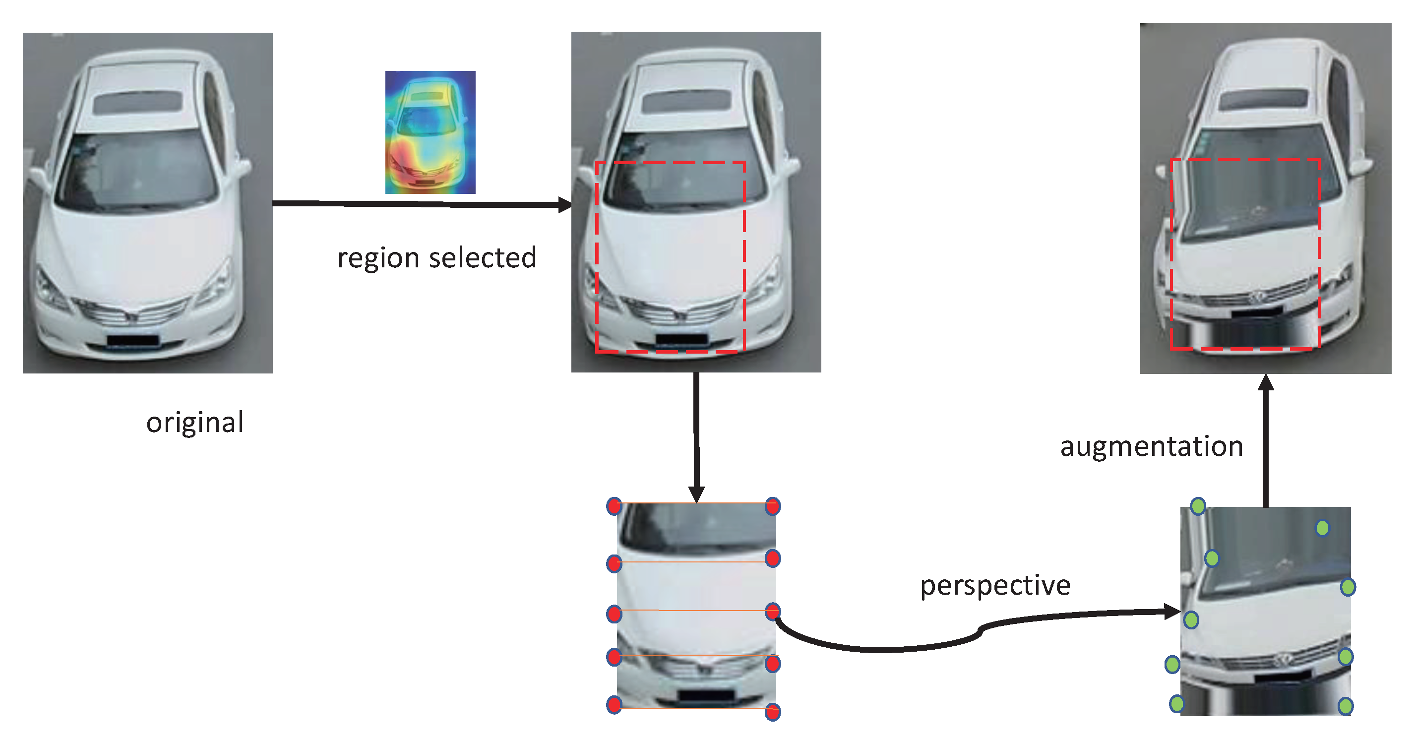
3.2. Salient Projection Region Location
| Algorithm 1: Salient Projection Region Location Procedure |
| Input: image P, area A, ratio of width and height R, area ratio ranging from to , aspect ratio ranging from to ; |
| Output: selected region |
| 1: |
| 2: |
| 3: |
| 4: |
| 5: |
| 6: |
| 7: |
| 8: SRA is Spatial Relation-Aware Attention [13]. The weight matrix W with rows and columns can be obtained from the SRA [13]. Obtain the weights. |
| 9: for i In do |
| 10: for j In do |
| 11: |
| 12: if then |
| 13: |
| 14: end if |
| 15: end for |
| 16: end for |
| 17: Use the loop to find the and its |
| 18: return region |
3.3. Local Region Projection Transformation
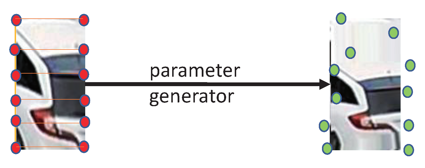
3.3.1. Parameter Agent Network
3.3.2. Projection Transformation
3.4. Transformation State Adversarial Module
| Algorithm 2: Adversarial Process of Parameter Agent Network (PAN) and Recognizer |
| Input: input image P, selected region A |
| Output: optimized |
| 1: sample transformation state from predicted distribution: |
| 2: generate random transformation states from to state , based on state |
| 3: all states including contain anchor points |
| 4: obtain augmented images from and based on states to state : |
| 5: The following i all represent 1 to 11 |
| 6: |
| 7: identify images: |
| 8: if then |
| 9: test distance between and |
| 10: if then |
| 11: = update with |
| 12: end if |
| 13: else |
| 14: = |
| 15: end if |
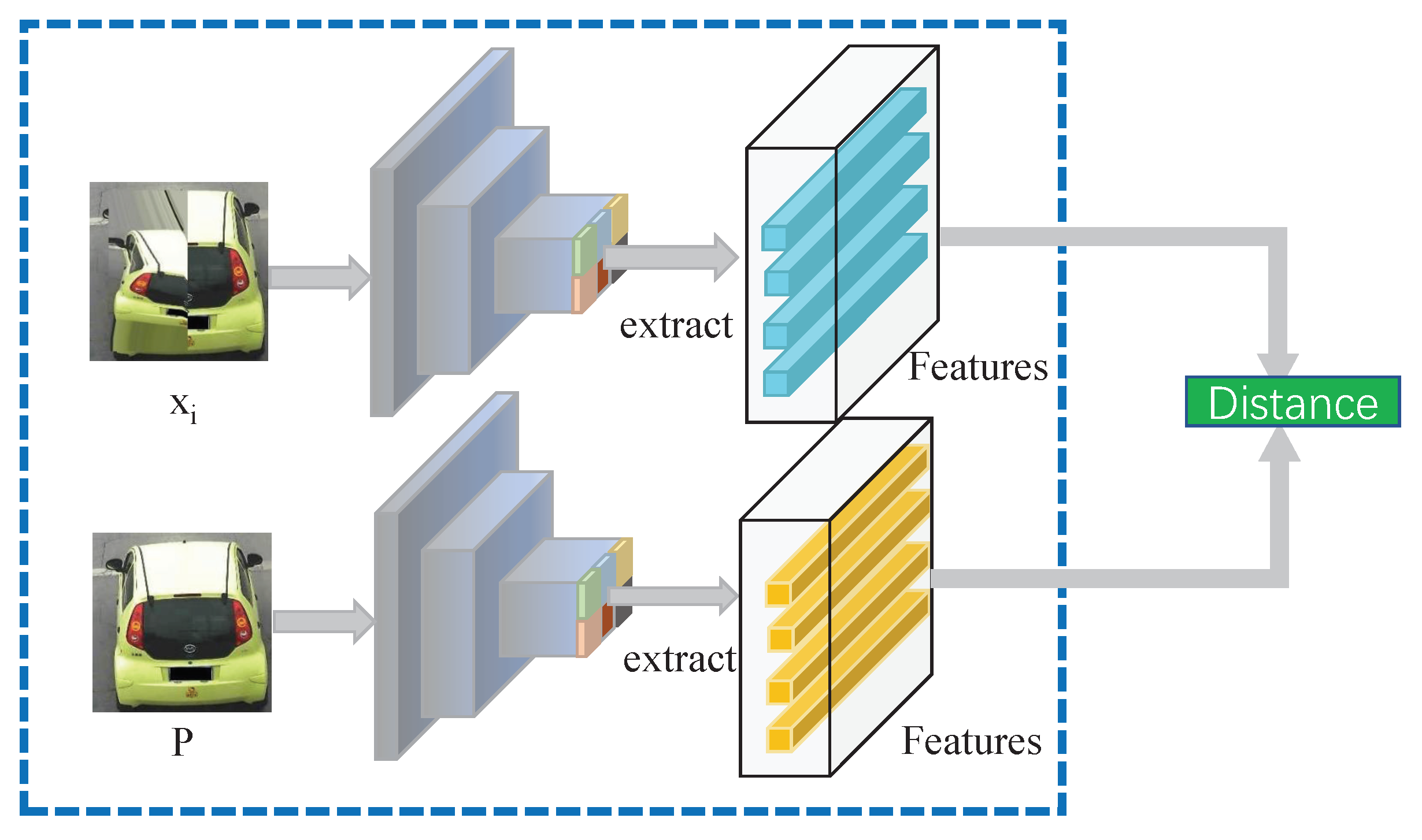
3.4.1. Recognizer
3.4.2. Learning Target Selection
4. Experiments and Discussion
4.1. Datasets
4.1.1. VehicleID
4.1.2. VeRi-776
4.1.3. VERI-Wild
4.2. Implementation
4.3. Ablation Study
4.3.1. Our Model vs. Baseline Model
4.3.2. Internal Comparison
4.4. Comparison with the SOTA
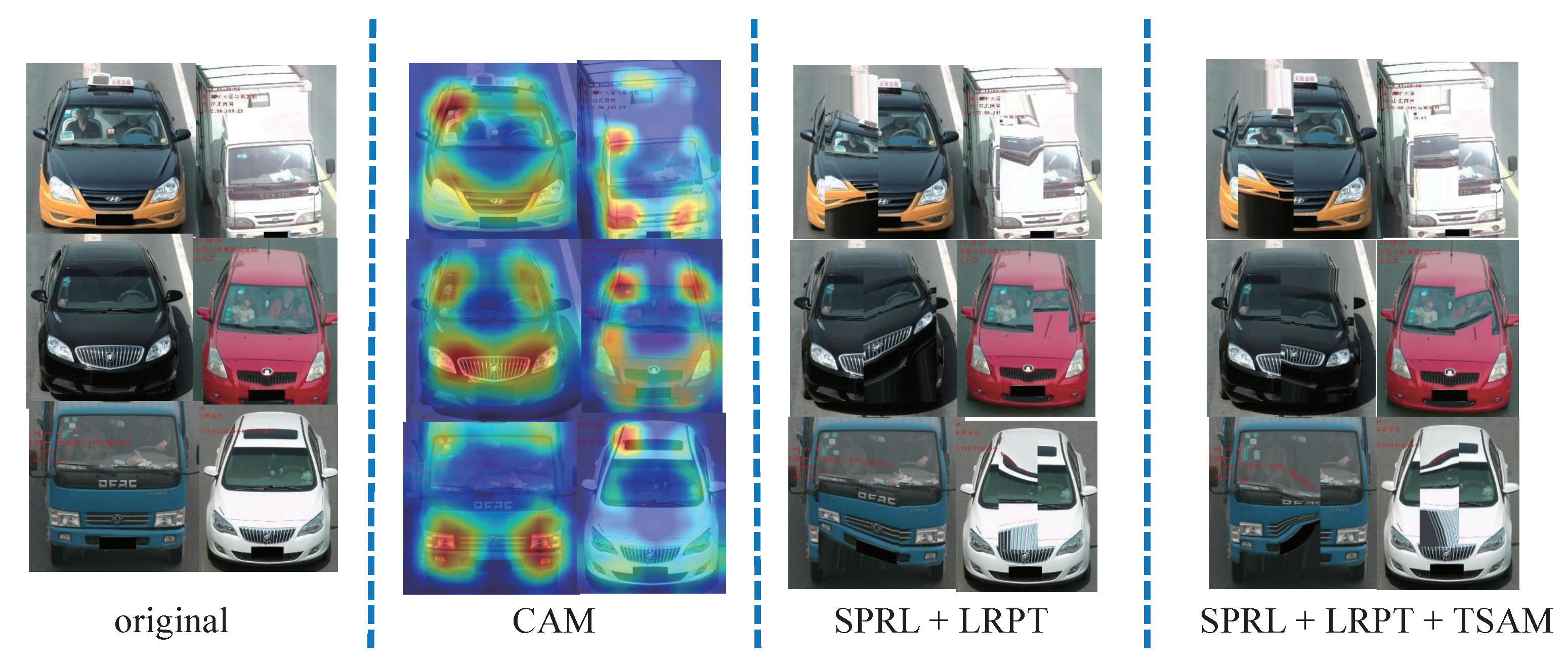
4.5. Visualization results
5. Conclusions
Author Contributions
Funding
Institutional Review Board Statement
Informed Consent Statement
Data Availability Statement
Acknowledgments
Conflicts of Interest
Abbreviations
| ReID | Re-Identification |
| SPRL | Salient Projection Region Location |
| LRPT | Local Region Projection Transformation |
| TSAM | Transformation State Adversarial Module |
| GAN | Generative Adversarial Networks |
| PAN | Parameter Agent Network |
Appendix A

| Symbol | Meaning |
|---|---|
| u | the pixel to be moved |
| t | the target’s moved position |
| M | the matrix having the property |
| the values within a range | |
| the weight of the 10 anchor points | |
| the weight of the 10 transformed anchor points |
References
- Li, J.; Cong, Y.; Zhou, L.; Tian, Z.; Qiu, J. Super-resolution-based part collaboration network for vehicle re-identification. World Wide Web 2022, 1–20. [Google Scholar] [CrossRef]
- Pan, B.; Qian, K.; Xie, H.; Asundi, A. Two-dimensional digital image correlation for in-plane displacement and strain measurement: A review. Meas. Sci. Technol. 2009, 20, 062001. [Google Scholar] [CrossRef]
- Xu, H.; Cai, Z.; Li, R.; Li, W. Efficient CityCam-to-Edge Cooperative Learning for Vehicle Counting in ITS. IEEE Trans. Intell. Transp. Syst. 2022, 23, 16600–16611. [Google Scholar] [CrossRef]
- Khan, S.D.; Ullah, H. A survey of advances in vision-based vehicle re-identification. Comput. Vis. Image Underst. 2019, 182, 50–63. [Google Scholar] [CrossRef]
- Rusk, N. Deep learning. Nat. Methods 2016, 13, 35. [Google Scholar] [CrossRef]
- Shorten, C.; Khoshgoftaar, T.M. A survey on image data augmentation for deep learning. J. Big Data 2019, 6, 60. [Google Scholar] [CrossRef]
- Xia, R.; Chen, Y.; Ren, B. Improved anti-occlusion object tracking algorithm using Unscented Rauch-Tung-Striebel smoother and kernel correlation filter. J. King Saud-Univ.-Comput. Inf. Sci. 2022, 34, 6008–6018. [Google Scholar] [CrossRef]
- Zhou, B.; Khosla, A.; Lapedriza, A.; Oliva, A.; Torralba, A. Learning deep features for discriminative localization. In Proceedings of the IEEE Conference on Computer Vision and Pattern Recognition, Las Vegas, NV, USA, 27–30 June 2016; pp. 2921–2929. [Google Scholar]
- Selvaraju, R.R.; Cogswell, M.; Das, A.; Vedantam, R.; Parikh, D.; Batra, D. Grad-cam: Visual explanations from deep networks via gradient-based localization. In Proceedings of the IEEE International Conference on Computer Vision, Venice, Italy, 22–29 October 2017; pp. 618–626. [Google Scholar]
- Chattopadhay, A.; Sarkar, A.; Howlader, P.; Balasubramanian, V.N. Grad-cam++: Generalized gradient-based visual explanations for deep convolutional networks. In Proceedings of the 2018 IEEE Winter Conference on Applications of Computer Vision (WACV), Lake Tahoe, NV, USA, 12–15 March 2018; pp. 839–847. [Google Scholar]
- Yang, W.; Huang, H.; Zhang, Z.; Chen, X.; Huang, K.; Zhang, S. Towards rich feature discovery with class activation maps augmentation for person re-identification. In Proceedings of the IEEE/CVF Conference on Computer Vision and Pattern Recognition, Long Beach, CA, USA, 16–20 June 2019; pp. 1389–1398. [Google Scholar]
- Zheng, M.; Karanam, S.; Wu, Z.; Radke, R.J. Re-identification with consistent attentive siamese networks. In Proceedings of the IEEE/CVF Conference on Computer Vision and Pattern Recognition, Long Beach, CA, USA, 16–20 June 2019; pp. 5735–5744. [Google Scholar]
- Zhang, Z.; Lan, C.; Zeng, W.; Jin, X.; Chen, Z. Relation-aware global attention. arXiv 2019, arXiv:1904.02998. [Google Scholar]
- Liu, X.; Liu, W.; Ma, H.; Fu, H. Large-scale vehicle re-identification in urban surveillance videos. In Proceedings of the 2016 IEEE International Conference on Multimedia and Expo (ICME), Seattle, WA, USA, 11–15 July 2016; pp. 1–6. [Google Scholar]
- Liu, H.; Tian, Y.; Yang, Y.; Pang, L.; Huang, T. Deep relative distance learning: Tell the difference between similar vehicles. In Proceedings of the IEEE Conference on Computer Vision and Pattern Recognition, Las Vegas, NV, USA, 27–30 June 2016; pp. 2167–2175. [Google Scholar]
- Lou, Y.; Bai, Y.; Liu, J.; Wang, S.; Duan, L. Veri-wild: A large dataset and a new method for vehicle re-identification in the wild. In Proceedings of the IEEE Conference on Computer Vision and Pattern Recognition, Long Beach, CA, USA, 16–20 June 2019; pp. 3235–3243. [Google Scholar]
- Zhang, J.; Feng, W.; Yuan, T.; Wang, J.; Sangaiah, A.K. SCSTCF: Spatial-channel selection and temporal regularized correlation filters for visual tracking. Appl. Soft Comput. 2022, 118, 108485. [Google Scholar] [CrossRef]
- Li, Y.; Li, Y.; Yan, H.; Liu, J. Deep joint discriminative learning for vehicle re-identification and retrieval. In Proceedings of the 2017 IEEE International Conference on Image Processing (ICIP), BeiJing, China, 17–20 September 2017; pp. 395–399. [Google Scholar]
- Shen, Y.; Xiao, T.; Li, H.; Yi, S.; Wang, X. Learning deep neural networks for vehicle re-id with visual-spatio-temporal path proposals. In Proceedings of the IEEE International Conference on Computer Vision, Venice, Italy, 22–29 October 2017; pp. 1900–1909. [Google Scholar]
- Wang, G.; Yuan, Y.; Chen, X.; Li, J.; Zhou, X. Learning discriminative features with multiple granularities for person re-identification. In Proceedings of the 26th ACM International Conference on Multimedia, Seoul, Republic of Korea, 22–26 October 2018; pp. 274–282. [Google Scholar]
- Stevenson, J.A.; Sun, X.; Mitchell, N.C. Despeckling SRTM and other topographic data with a denoising algorithm. Geomorphology 2010, 114, 238–252. [Google Scholar] [CrossRef]
- Teng, S.; Liu, X.; Zhang, S.; Huang, Q. Scan: Spatial and channel attention network for vehicle re-identification. In Pacific Rim Conference on Multimedia; Springer: Berlin/Heidelberg, Germany, 2018; pp. 350–361. [Google Scholar]
- Zhou, T.; Tulsiani, S.; Sun, W.; Malik, J.; Efros, A.A. View synthesis by appearance flow. In European Conference on Computer Vision; Springer: Berlin/Heidelberg, Germany, 2016. [Google Scholar]
- Isola, P.; Zhu, J.Y.; Zhou, T.; Efros, A.A. Image-to-image translation with conditional adversarial networks. In Proceedings of the IEEE Conference on Computer Vision and Pattern Recognition, Honolulu, HI, USA, 21–26 July 2017; pp. 1125–1134. [Google Scholar]
- Johnson, J.; Alahi, A.; Fei-Fei, L. Perceptual losses for real-time style transfer and super-resolution. In European Conference on Computer Vision; Springer: Berlin/Heidelberg, Germany, 2016; pp. 694–711. [Google Scholar]
- Odena, A.; Olah, C.; Shlens, J. Conditional image synthesis with auxiliary classifier gans. In Proceedings of the International Conference on Machine Learning, PMLR, Sydney, Australia, 6–11 August 2017; pp. 2642–2651. [Google Scholar]
- Goodfellow, I.; Pouget-Abadie, J.; Mirza, M.; Xu, B.; Warde-Farley, D.; Ozair, S.; Courville, A.; Bengio, Y. Generative adversarial nets. Adv. Neural Inf. Process. Syst. 2014, 27, 2672–2680. [Google Scholar]
- Bowles, C.; Chen, L.; Guerrero, R.; Bentley, P.; Gunn, R.; Hammers, A.; Dickie, D.A.; Hernández, M.V.; Wardlaw, J.; Rueckert, D. Gan augmentation: Augmenting training data using generative adversarial networks. arXiv 2018, arXiv:1810.10863. [Google Scholar]
- Radford, A.; Metz, L.; Chintala, S. Unsupervised representation learning with deep convolutional generative adversarial networks. arXiv 2015, arXiv:1511.06434. [Google Scholar]
- Zhu, X.; Liu, Y.; Li, J.; Wan, T.; Qin, Z. Emotion classification with data augmentation using generative adversarial networks. In Pacific-Asia Conference on Knowledge Discovery and Data Mining; Springer: Berlin/Heidelberg, Germany, 2018; pp. 349–360. [Google Scholar]
- Ruder, S. An overview of multi-task learning in deep neural networks. arXiv 2017, arXiv:1706.05098. [Google Scholar]
- Luo, H.; Chen, W.; Xu, X.; Gu, J.; Li, H. An Empirical Study of Vehicle Re-Identification on the AI City Challenge. Available online: https://arxiv.org/abs/2105.09701 (accessed on 20 October 2022).
- Melekhov, I.; Kannala, J.; Rahtu, E. Siamese network features for image matching. In Proceedings of the 2016 23rd International Conference on Pattern Recognition (ICPR), Cancun, Mexico, 4–8 December 2016; pp. 378–383. [Google Scholar]
- Wang, W.; Zheng, V.W.; Yu, H.; Miao, C. A survey of zero-shot learning: Settings, methods, and applications. ACM Trans. Intell. Syst. Technol. 2019, 10, 1–37. [Google Scholar] [CrossRef]
- Schaefer, S.; McPhail, T.; Warren, J. Image deformation using moving least squares. In Proceedings of the ACM SIGGRAPH: Applied Perception in Graphics & Visualization 2006 Papers, New York, NY, USA, 30 July–3 August 2006; pp. 533–540. [Google Scholar]
- Chan, K.H.; Ke, W.; Im, S.K. A General Method for Generating Discrete Orthogonal Matrices. IEEE Access 2021, 9, 120380–120391. [Google Scholar] [CrossRef]
- He, K.; Zhang, X.; Ren, S.; Sun, J. Deep residual learning for image recognition. In Proceedings of the IEEE Conference on Computer Vision and Pattern Recognition, Caesar’s Palace, Las Vegas, NV, USA, 26 June–1 July 2016; pp. 770–778. [Google Scholar]
- Krizhevsky, A.; Sutskever, I.; Hinton, G.E. Imagenet classification with deep convolutional neural networks. Adv. Neural Inf. Process. Syst. 2012, 25, 1097–1105. [Google Scholar] [CrossRef]
- Deng, J.; Dong, W.; Socher, R.; Li, L.J.; Li, K.; Fei-Fei, L. Imagenet: A large-scale hierarchical image database. In Proceedings of the 2009 IEEE Conference on Computer Vision And Pattern Recognition, Miami, FL, USA, 20–25 June 2009; pp. 248–255. [Google Scholar]
- Jung, H.; Choi, M.K.; Jung, J.; Lee, J.H.; Kwon, S.; Young Jung, W. ResNet-based vehicle classification and localization in traffic surveillance systems. In Proceedings of the IEEE Conference on Computer Vision and Pattern Recognition Workshops, the Hawaii Convention Center, Honolulu, HI, USA, 21–26 July 2017; pp. 61–67. [Google Scholar]
- Zhang, S.; Choromanska, A.; LeCun, Y. Deep learning with elastic averaging SGD. arXiv 2014, arXiv:1412.6651. [Google Scholar]
- Yuan, Y.; Chen, W.; Yang, Y.; Wang, Z. In defense of the triplet loss again: Learning robust person re-identification with fast approximated triplet loss and label distillation. In Proceedings of the IEEE/CVF Conference on Computer Vision and Pattern Recognition Workshops, Online, 14–19 July 2020; pp. 354–355. [Google Scholar]
- He, S.; Luo, H.; Chen, W.; Zhang, M.; Zhang, Y.; Wang, F.; Li, H.; Jiang, W. Multi-domain learning and identity mining for vehicle re-identification. In Proceedings of the IEEE/CVF Conference on Computer Vision and Pattern Recognition Workshops, Online, 14–19 July 2020; pp. 582–583. [Google Scholar]
- Luo, H.; Gu, Y.; Liao, X.; Lai, S.; Jiang, W. Bag of tricks and a strong baseline for deep person re-identification. In Proceedings of the IEEE/CVF Conference on Computer Vision and Pattern Recognition Workshops, Long Beach, CA, USA, 16–20 July 2019. [Google Scholar]
- Luo, H.; Jiang, W.; Gu, Y.; Liu, F.; Liao, X.; Lai, S.; Gu, J. A strong baseline and batch normalization neck for deep person re-identification. IEEE Trans. Multimed. 2019, 22, 2597–2609. [Google Scholar] [CrossRef]
- Liu, X.; Liu, W.; Mei, T.; Ma, H. Provid: Progressive and multimodal vehicle reidentification for large-scale urban surveillance. IEEE Trans. Multimed. 2017, 20, 645–658. [Google Scholar] [CrossRef]
- Khorramshahi, P.; Kumar, A.; Peri, N.; Rambhatla, S.S.; Chen, J.C.; Chellappa, R. A dual-path model with adaptive attention for vehicle re-identification. In Proceedings of the IEEE International Conference on Computer Vision, Seoul, Republic of Korea, 27 October–2 November 2019; pp. 6132–6141. [Google Scholar]
- Kuma, R.; Weill, E.; Aghdasi, F.; Sriram, P. Vehicle re-identification: An efficient baseline using triplet embedding. In Proceedings of the 2019 International Joint Conference on Neural Networks (IJCNN), Budapest, Hungary, 14–19 July 2019; pp. 1–9. [Google Scholar]
- Peng, J.; Jiang, G.; Chen, D.; Zhao, T.; Wang, H.; Fu, X. Eliminating cross-camera bias for vehicle re-identification. Multimed. Tools Appl. 2020, 81, 34195–34211. [Google Scholar] [CrossRef]
- He, B.; Li, J.; Zhao, Y.; Tian, Y. Part-regularized near-duplicate vehicle re-identification. In Proceedings of the IEEE Conference on Computer Vision and Pattern Recognition, Long Beach, CA, USA, 16–20 July 2019; pp. 3997–4005. [Google Scholar]
- Zheng, A.; Lin, X.; Li, C.; He, R.; Tang, J. Attributes guided feature learning for vehicle re-identification. arXiv 2019, arXiv:1905.08997. [Google Scholar]
- Tang, Z.; Naphade, M.; Birchfield, S.; Tremblay, J.; Hodge, W.; Kumar, R.; Wang, S.; Yang, X. Pamtri: Pose-aware multi-task learning for vehicle re-identification using highly randomized synthetic data. In Proceedings of the IEEE International Conference on Computer Vision, the COEX Convention Center, Seoul, Republic of Korea, 27 October–2 November 2019; pp. 211–220. [Google Scholar]
- Yao, Y.; Zheng, L.; Yang, X.; Naphade, M.; Gedeon, T. Simulating content consistent vehicle datasets with attribute descent. arXiv 2019, arXiv:1912.08855. [Google Scholar]
- Zhou, Y.; Shao, L. Aware attentive multi-view inference for vehicle re-identification. In Proceedings of the IEEE Conference on Computer Vision and Pattern Recognition, the Calvin L. Rampton Salt Palace Convention Center, Salt Lake City, UT, USA, 18–22 June 2018; pp. 6489–6498. [Google Scholar]
- Wang, Z.; Tang, L.; Liu, X.; Yao, Z.; Yi, S.; Shao, J.; Yan, J.; Wang, S.; Li, H.; Wang, X. Orientation invariant feature embedding and spatial temporal regularization for vehicle re-identification. In Proceedings of the IEEE International Conference on Computer Vision, Venice, Italy, 22–29 October 2017; pp. 379–387. [Google Scholar]
- Yang, L.; Luo, P.; Change Loy, C.; Tang, X. A large-scale car dataset for fine-grained categorization and verification. In Proceedings of the IEEE Conference on Computer Vision and Pattern Recognition, Boston, MA, USA, 7–12 June 2015; pp. 3973–3981. [Google Scholar]
- Alfasly, S.; Hu, Y.; Li, H.; Liang, T.; Jin, X.; Liu, B.; Zhao, Q. Multi-Label-Based Similarity Learning for Vehicle Re-Identification. IEEE Access 2019, 7, 162605–162616. [Google Scholar] [CrossRef]


| Module | Type |
|---|---|
| Initial | |
| Conv16, ReLU, MP | |
| Conv64, ReLU, MP | |
| Conv128, BN, ReLU | |
| Conv128, ReLU, MP | |
| Conv64, BN, ReLU | |
| Conv16, BN, ReLU, MP | |
| FC Layer |
| Models | VehicleID | VERI-Wild | ||||||||||||
|---|---|---|---|---|---|---|---|---|---|---|---|---|---|---|
| VeRi-776 | Small | Medium | Large | Small | Medium | Large | ||||||||
| Rank1 | MAP | Rank1 | MAP | Rank1 | MAP | Rank1 | MAP | Rank1 | MAP | Rank1 | MAP | Rank1 | MAP | |
| Baseline | 95.71 | 76.59 | 83.02 | 77.02 | 80.74 | 75.04 | 79.24 | 73.98 | 93.11 | 72.60 | 90.54 | 66.51 | 86.40 | 58.52 |
| SPRL + LRPT (Ours) | 96.66 | 80.5 | 84.26 | 77.8 | 83.38 | 77.9 | 79.91 | 74.44 | 91.81 | 72.73 | 90.38 | 66.64 | 87.66 | 58.73 |
| SPRL + LRPT + TSAM (Ours) | 96.84 | 81.55 | 84.34 | 77.85 | 83.42 | 77.96 | 79.96 | 74.52 | 93.31 | 72.75 | 91.03 | 66.68 | 87.7 | 58.78 |
| Models | MAP | Rank1 | Rank5 |
|---|---|---|---|
| siameseCNN [19] | 54.20 | 79.30 | 88.90 |
| fdaNet [16] | 55.50 | 84.30 | 92.40 |
| siameseCNN+ST [19] | 58.30 | 83.50 | 90.00 |
| provid [46] | 53.40 | 81.60 | 95.10 |
| aaver [47] | 66.35 | 90.17 | 94.34 |
| bs [48] | 67.55 | 90.23 | 96.42 |
| cca [49] | 68.05 | 91.71 | 94.34 |
| prn [50] | 70.20 | 92.20 | 97.90 |
| agNet [51] | 71.59 | 95.61 | 96.56 |
| pamtri [52] | 71.80 | 92.90 | 97.00 |
| vehicleX [53] | 73.26 | 94.99 | 97.97 |
| mdl [43] | 79.40 | 90.70 | - |
| ours | 81.55 | 96.84 | 98.99 |
| Models | Small | Medium | Large | |||
|---|---|---|---|---|---|---|
| Rank1 | Rank5 | Rank1 | Rank5 | Rank1 | Rank5 | |
| vami [54] | 63.10 | 83.30 | 52.90 | 75.10 | 47.30 | 70.30 |
| fdaNet [16] | - | - | 59.80 | 77.10 | 55.50 | 74.70 |
| agNet [51] | 71.15 | 83.78 | 69.23 | 81.41 | 65.74 | 78.28 |
| aaver [47] | 74.70 | 93.80 | 68.60 | 90.00 | 63.50 | 85.60 |
| oife [55] | - | - | - | - | 67.00 | 82.90 |
| cca [49] | 75.51 | 91.14 | 73.60 | 86.46 | 70.08 | 83.20 |
| prn [50] | 78.40 | 92.3 | 75.00 | 88.30 | 74.20 | 86.40 |
| bs [48] | 78.80 | 96.17 | 73.41 | 92.57 | 69.33 | 89.45 |
| vehicleX [53] | 79.81 | 93.17 | 76.74 | 90.34 | 73.88 | 88.18 |
| ours | 84.34 | 93.48 | 83.42 | 90.63 | 79.96 | 86.52 |
| Models | Small | Medium | Large | |||
|---|---|---|---|---|---|---|
| MAP | Rank1 | MAP | Rank1 | MAP | Rank1 | |
| googLeNet [56] | 24.30 | 57.20 | 24.20 | 53.20 | 21.50 | 44.60 |
| fdaNet [16] | 35.10 | 64.00 | 29.80 | 57.80 | 22.80 | 49.40 |
| mlsl [57] | 46.30 | 86.00 | 42.40 | 83.00 | 36.60 | 77.50 |
| aaver [47] | 62.23 | 75.80 | 53.66 | 68.24 | 41.68 | 58.69 |
| bs [48] | 70.05 | 84.17 | 62.83 | 78.22 | 51.63 | 69.99 |
| ours | 72.75 | 93.31 | 66.68 | 91.03 | 58.78 | 87.70 |
Publisher’s Note: MDPI stays neutral with regard to jurisdictional claims in published maps and institutional affiliations. |
© 2022 by the authors. Licensee MDPI, Basel, Switzerland. This article is an open access article distributed under the terms and conditions of the Creative Commons Attribution (CC BY) license (https://creativecommons.org/licenses/by/4.0/).
Share and Cite
Chen, Y.; Ke, W.; Zhang, W.; Wang, C.; Sheng, H.; Xiong, Z. Learning for Data Synthesis: Joint Local Salient Projection and Adversarial Network Optimization for Vehicle Re-Identification. Sensors 2022, 22, 9539. https://doi.org/10.3390/s22239539
Chen Y, Ke W, Zhang W, Wang C, Sheng H, Xiong Z. Learning for Data Synthesis: Joint Local Salient Projection and Adversarial Network Optimization for Vehicle Re-Identification. Sensors. 2022; 22(23):9539. https://doi.org/10.3390/s22239539
Chicago/Turabian StyleChen, Yanbing, Wei Ke, Wei Zhang, Cui Wang, Hao Sheng, and Zhang Xiong. 2022. "Learning for Data Synthesis: Joint Local Salient Projection and Adversarial Network Optimization for Vehicle Re-Identification" Sensors 22, no. 23: 9539. https://doi.org/10.3390/s22239539
APA StyleChen, Y., Ke, W., Zhang, W., Wang, C., Sheng, H., & Xiong, Z. (2022). Learning for Data Synthesis: Joint Local Salient Projection and Adversarial Network Optimization for Vehicle Re-Identification. Sensors, 22(23), 9539. https://doi.org/10.3390/s22239539