
Deep Learning Based Infrared Thermal Image Analysis of Complex Pavement Defect Conditions Considering Seasonal Effect


Abstract
1. Introduction
- This deep learning algorithm categorises pavement features accurately irrespective of the weather season to illustrate the feasibility of replacing one image type with other beneficially.
- Sunny conditions during summer and winter presented prediction accuracy for DC images, followed by MSX and then IR-T.
- An inexpensive IR-T imaging camera with medium resolution level can be economical, unlike expensive alternate options; however, its usage is limited to summer sunny conditions.
2. Materials and Methods
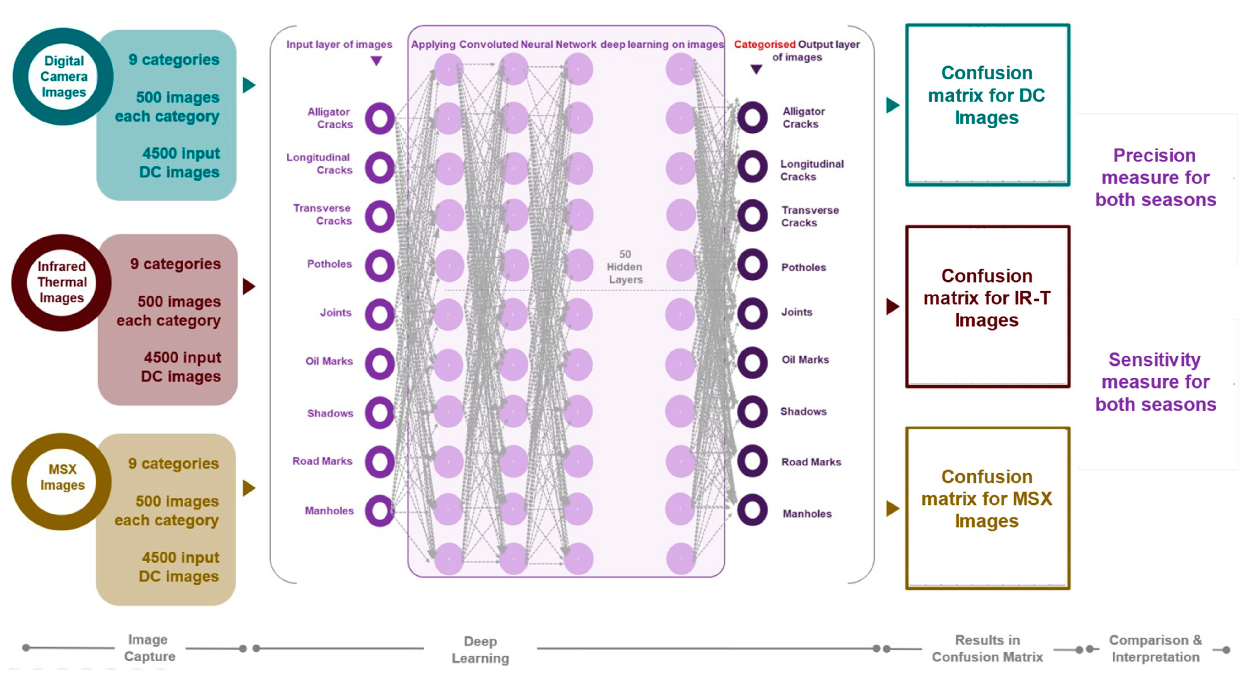
2.1. Overall Procedure
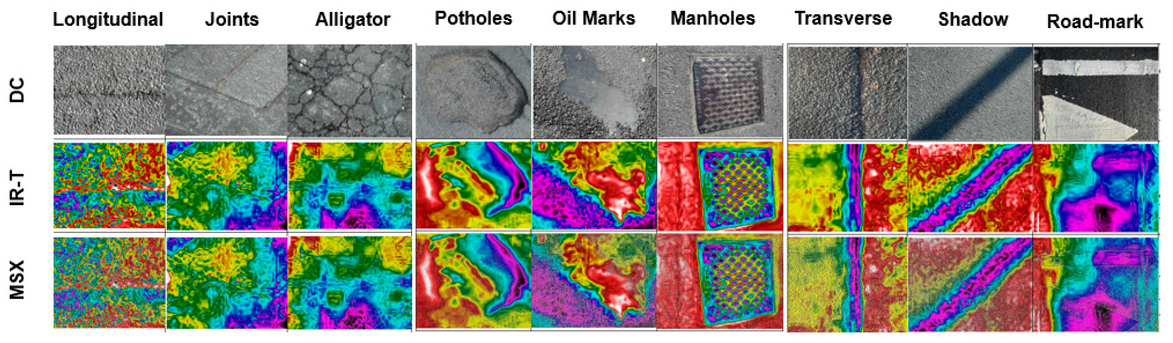
2.2. Experimental Setup and Data Collection
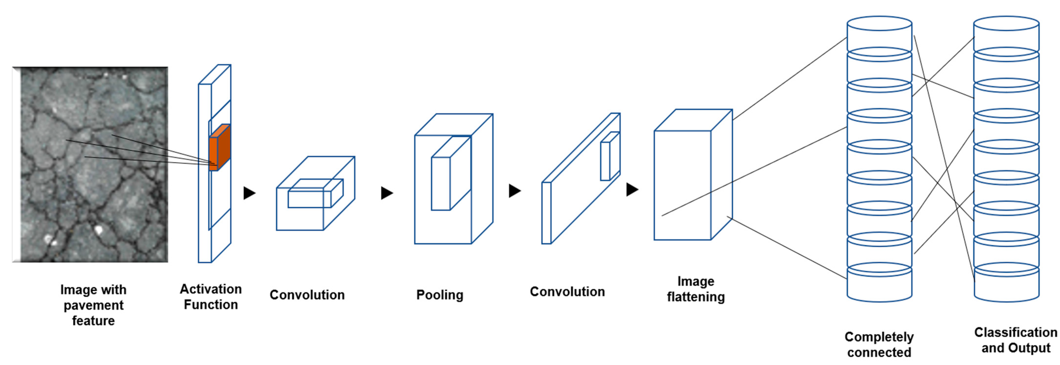
2.3. Data Augmentation, Multi Spectral Dynamic Imaging (MSX) and Test/Training Algorithm
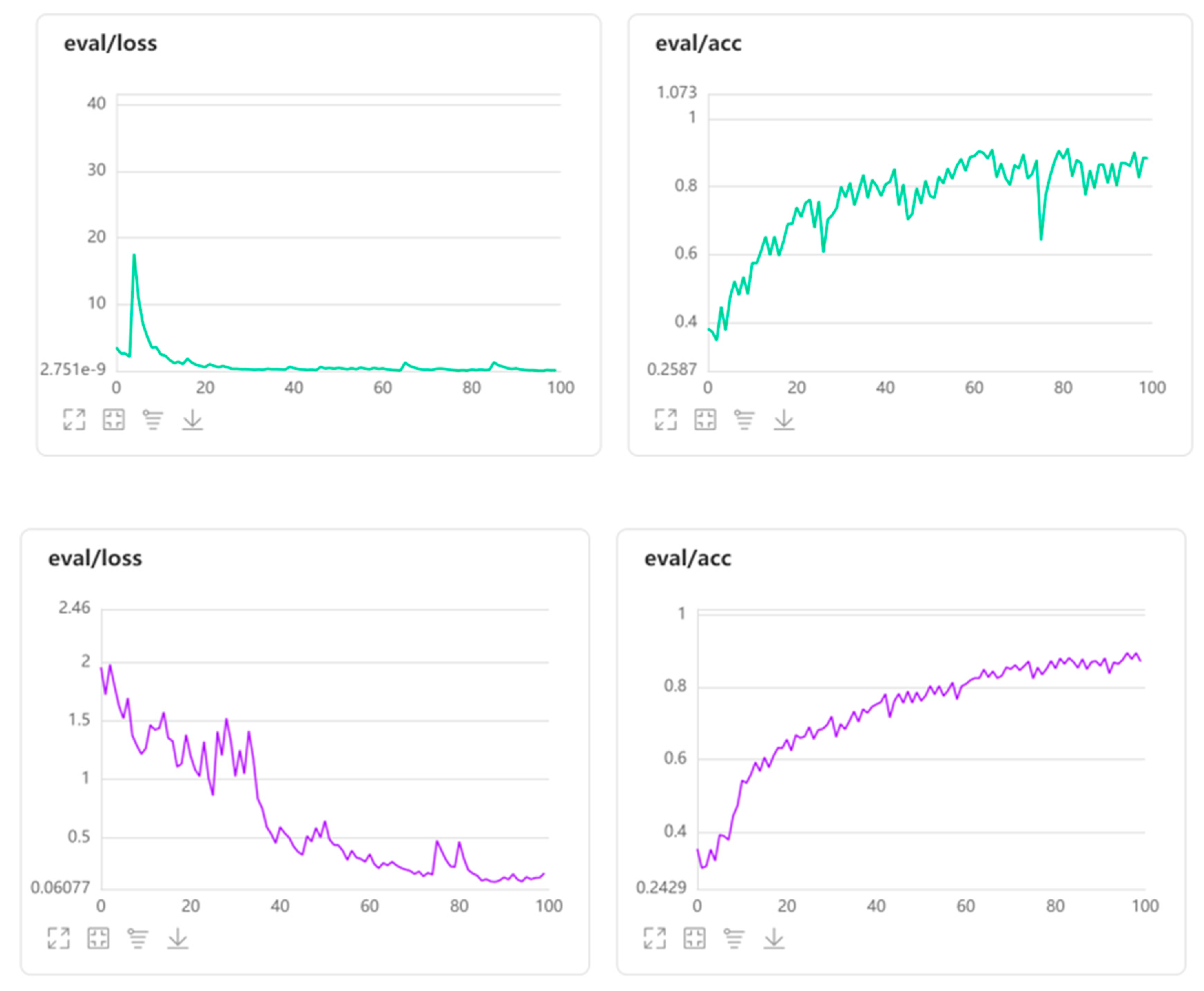
- Convolution layers: The number of layers within each image that will be assessed for feature extractions. Fifty layers were employed for this assessment,Loss function type: The convergence of the prediction with ideal output. The cross-entropy loss type was employed for this assessment. This loss function measures the level of deviation between the prediction and the actual image. Specifically, this measures loss as log loss (y-axis) that handles two different probabilistic distributions. Evidently, the higher the log loss, the higher the distinction between the probability distributions.Performing this on the summer conditions data, the profile for all three image types exhibited a converse nature of losses with the accuracy profile and the level of deviation drops (converges) for all three image types. Commencing at a high logarithmic scale of error, the level of convergence reached 0.039, 0.098 and 0.163 for DC, IR-T and MSX image types, respectively, as the model’s learning progressed.
- Epoch: Refers to the number of times the algorithm puts a test (or evaluation) image through the training data (higher passes results in better results). A hundred epoch passes were employed for this assessment,
- Batch size: Each epoch pass is executed within an interior loop enabling a batch of on input image processed. A batch size of 48 was employed for this assessment,
- Optimiser: Application of statistical optimization approach for convergence. A stochastic/paddle type optimiser was employed for this assessment, and
- Momentum: Parameter that dictates the subsequent step’s direction from the current step (preventing back and forth oscillations), usually a slope measure. A momentum of 0.9 was employed for this assessment.
3. Results
3.1. Evaluation Metrics
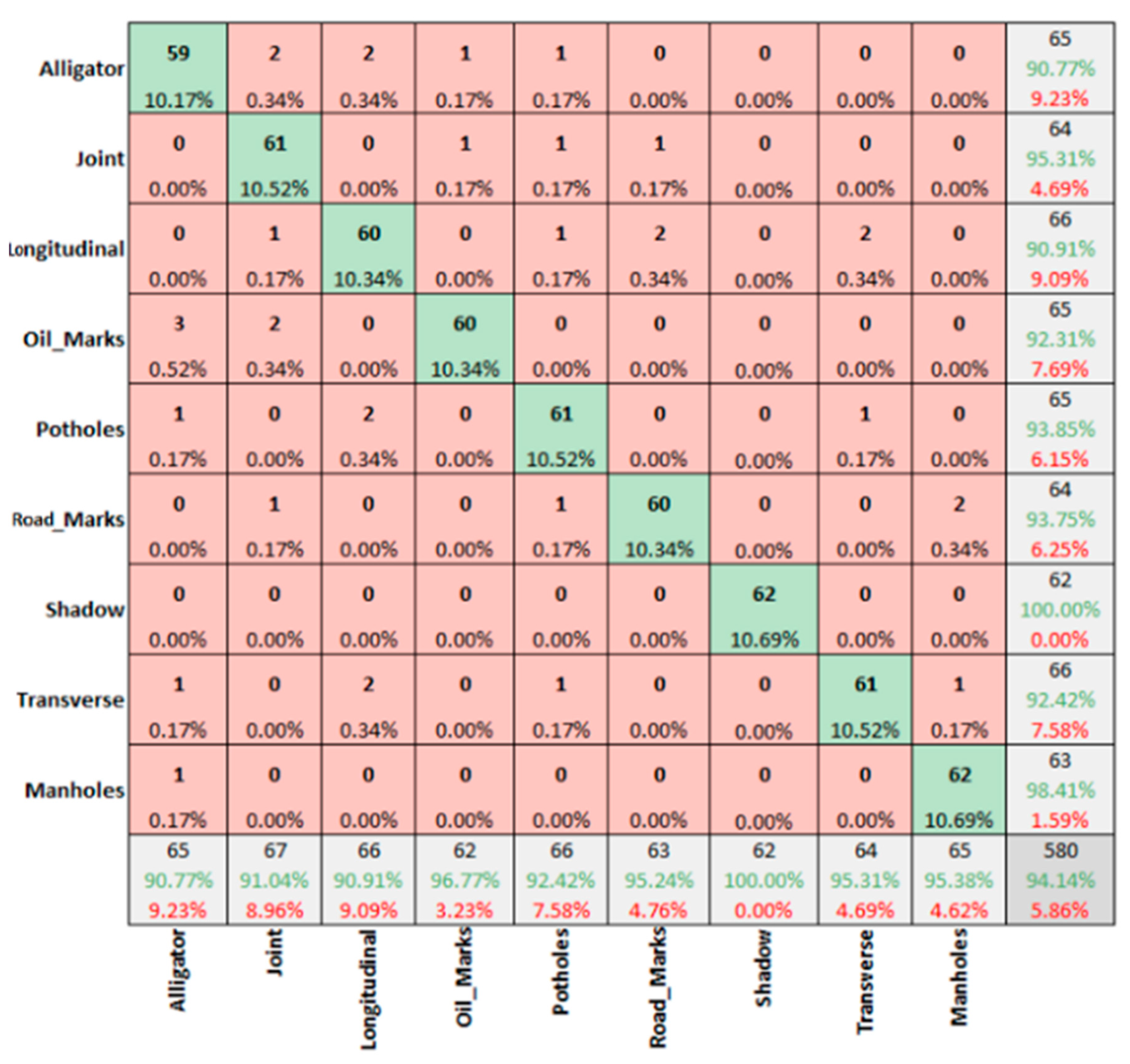
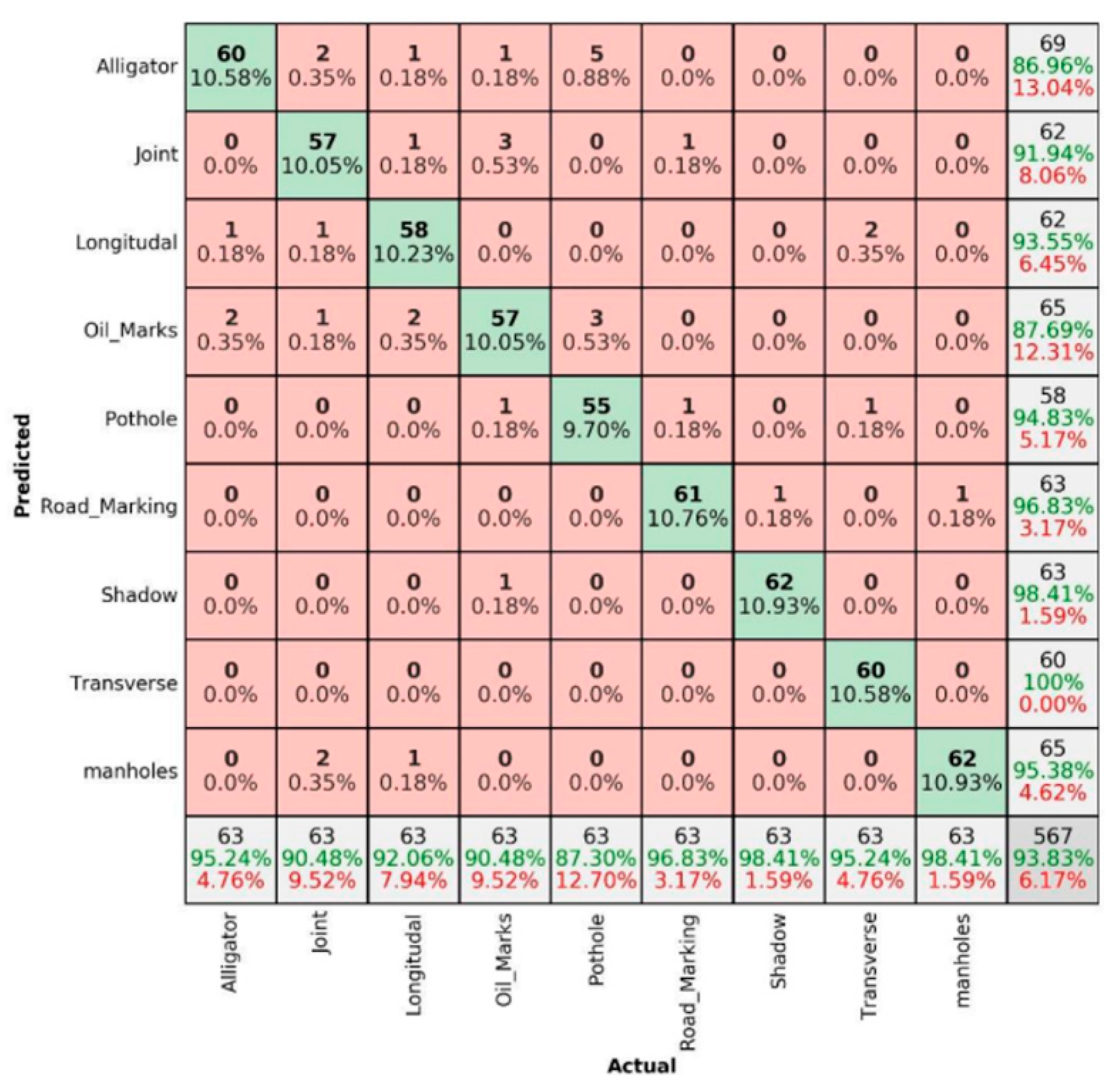
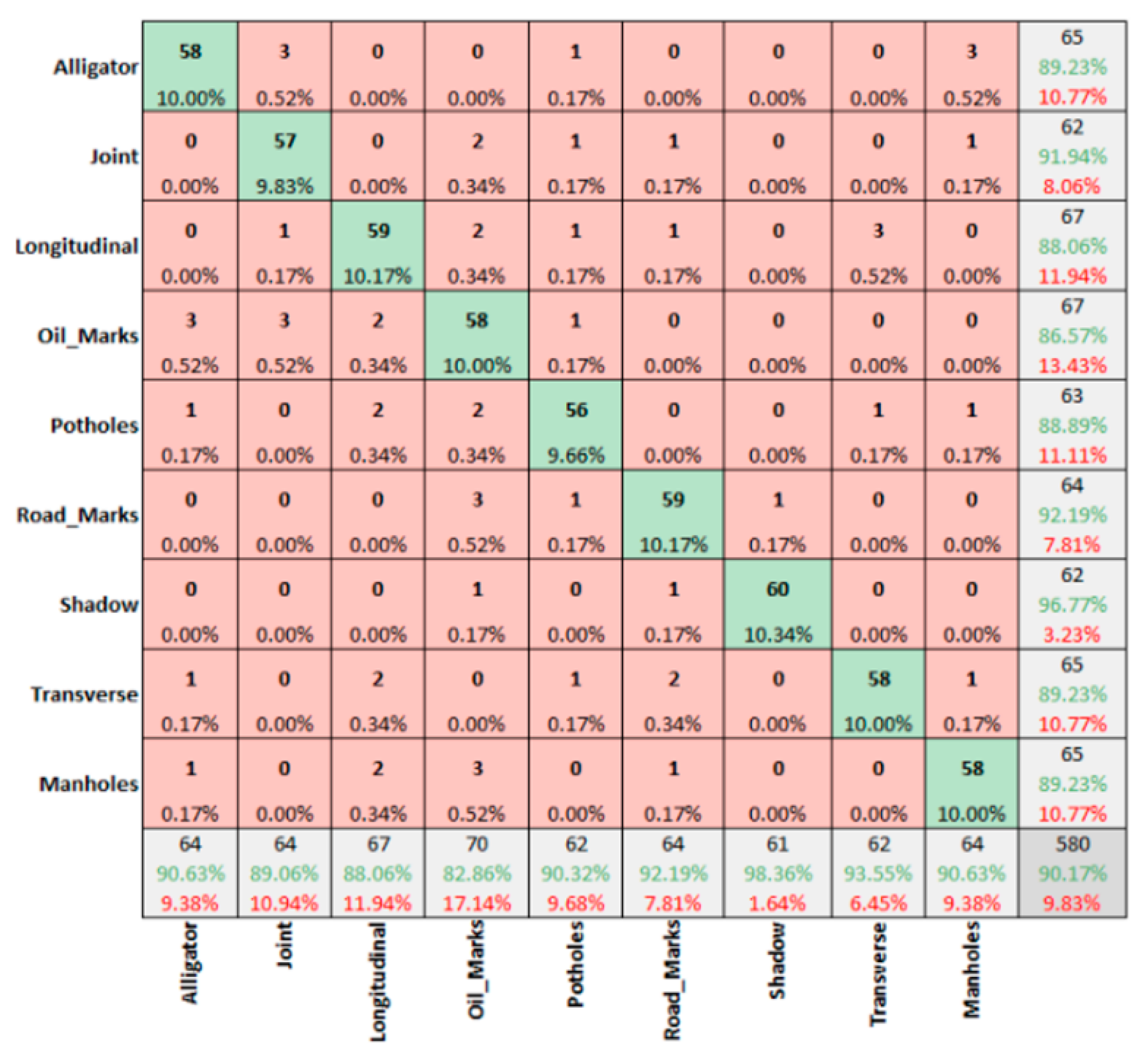
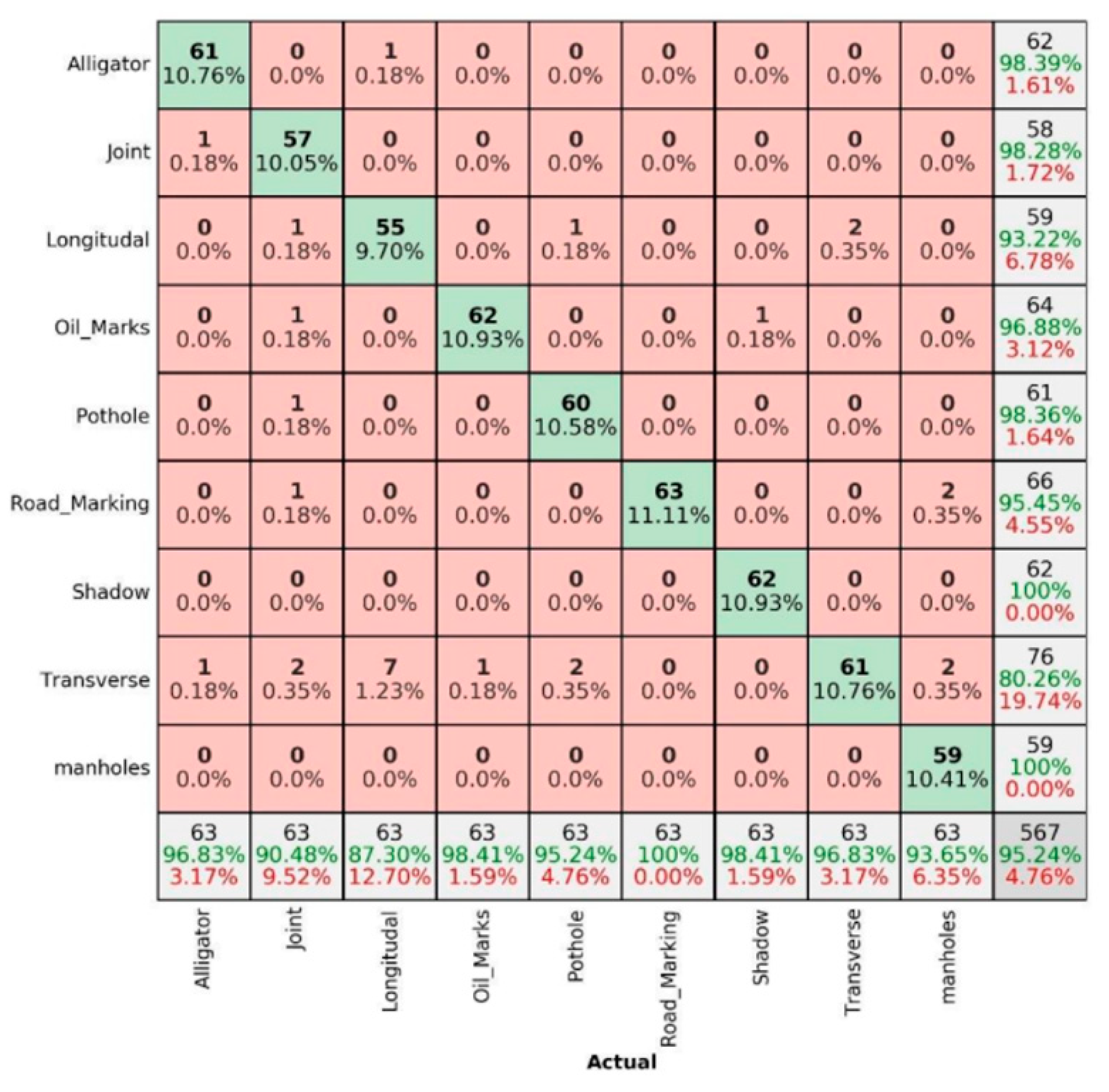
3.2. Comparing of Confusion Matrices for Summer and Winter Season in Sunny Conditions
4. Discussion
5. Conclusions
- The deep learning algorithm categorises pavement features (both damages and non-damages) around 92% accurately (95.18% in summer and 91.67% in winter conditions) irrespective of the weather season to illustrate the feasibility of replacing one image type with the other beneficially. Additionally, despite limited resolution, higher accuracy levels can be attained by providing the algorithm with more learning opportunities through a large input dataset.
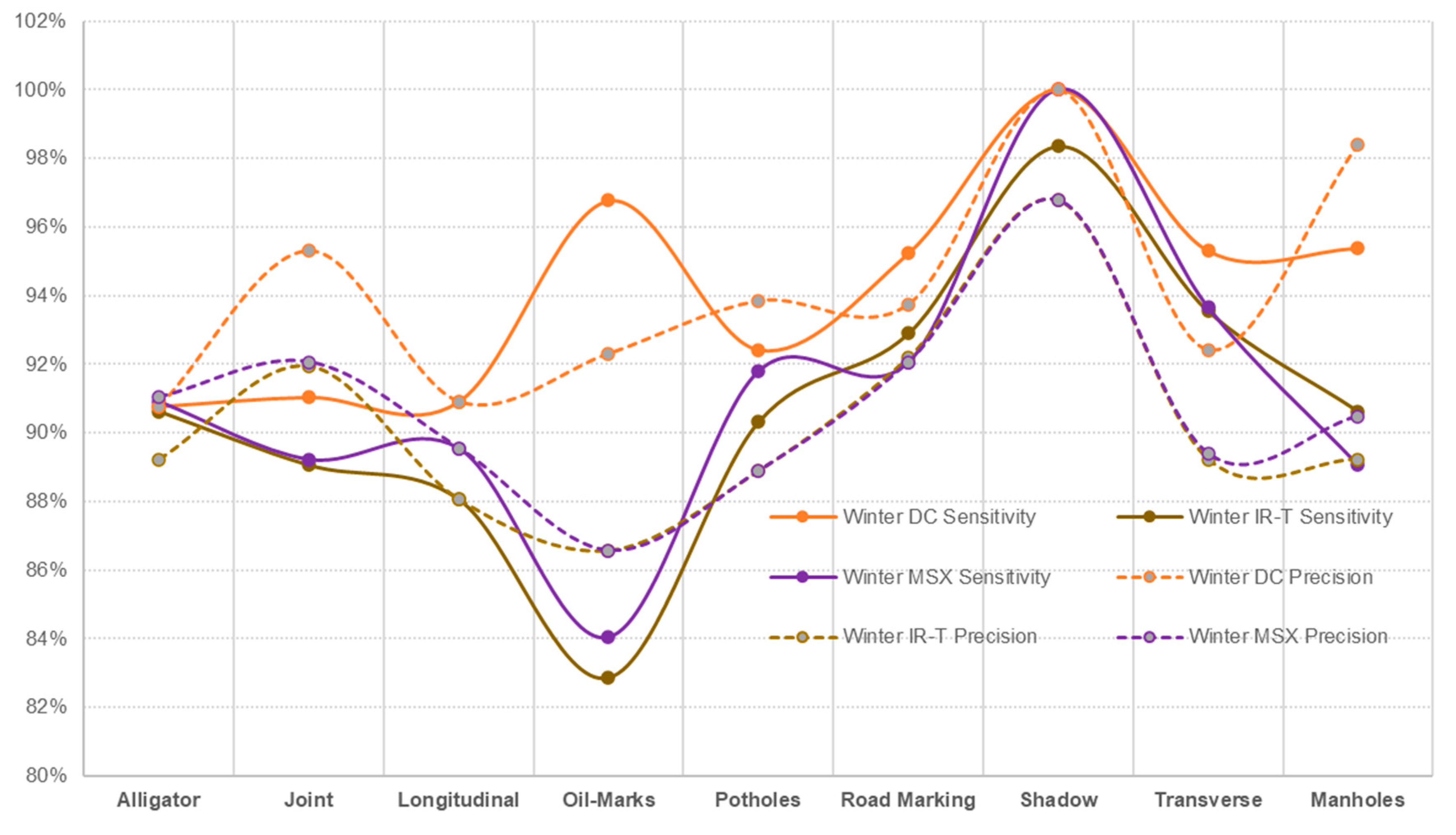
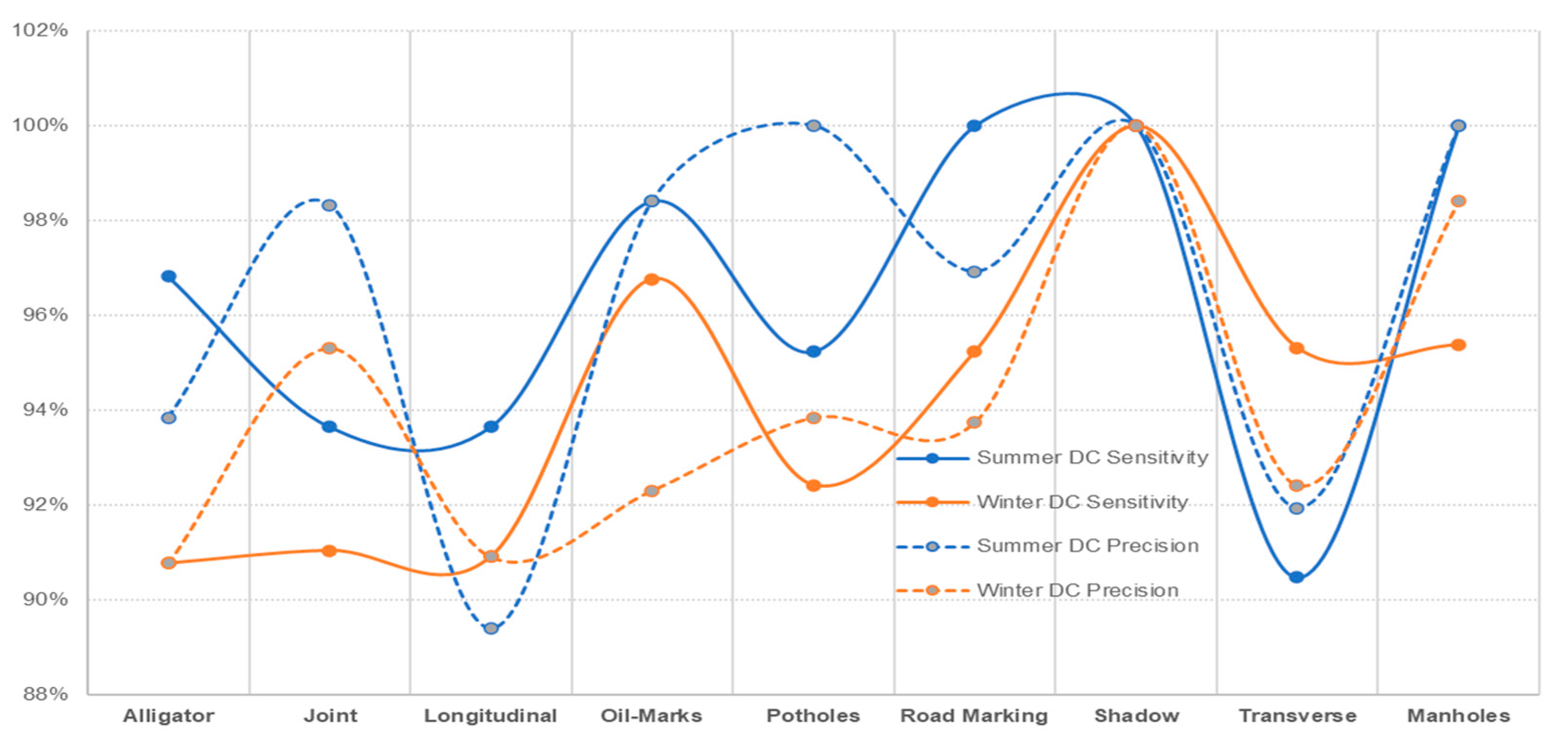
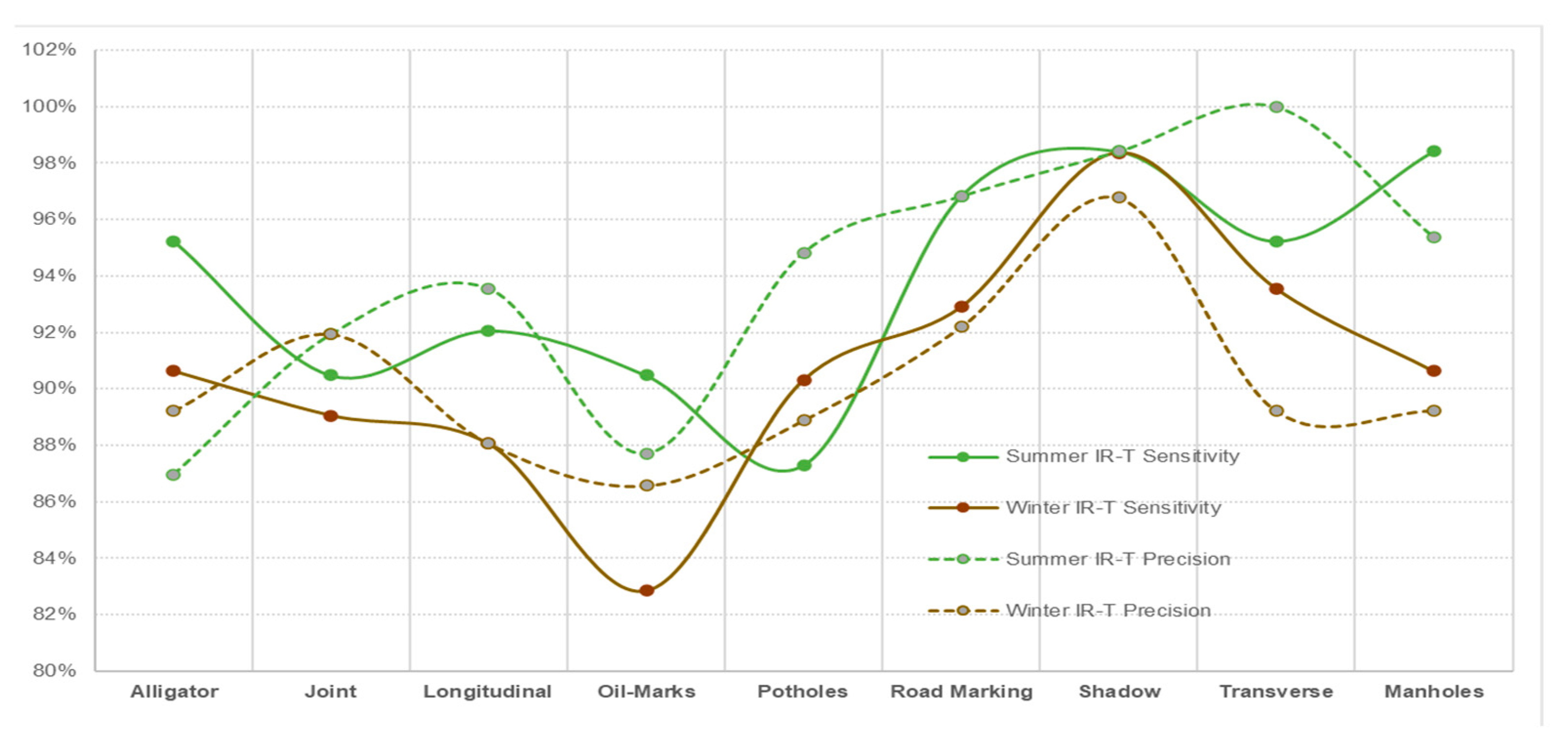
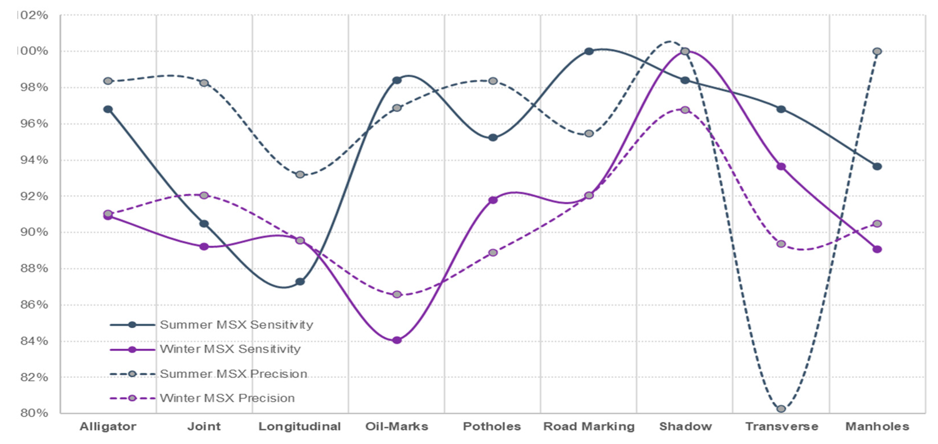
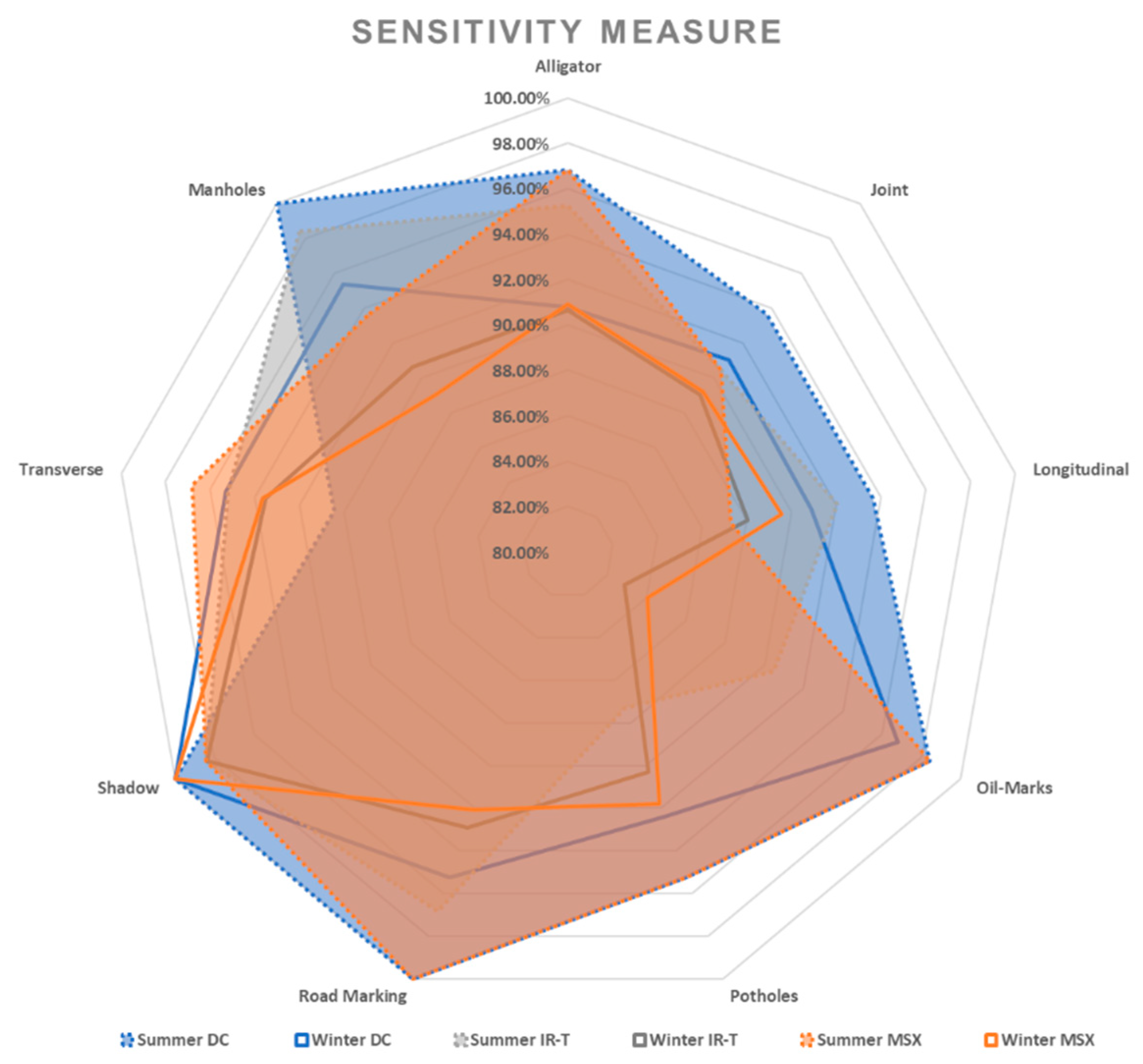
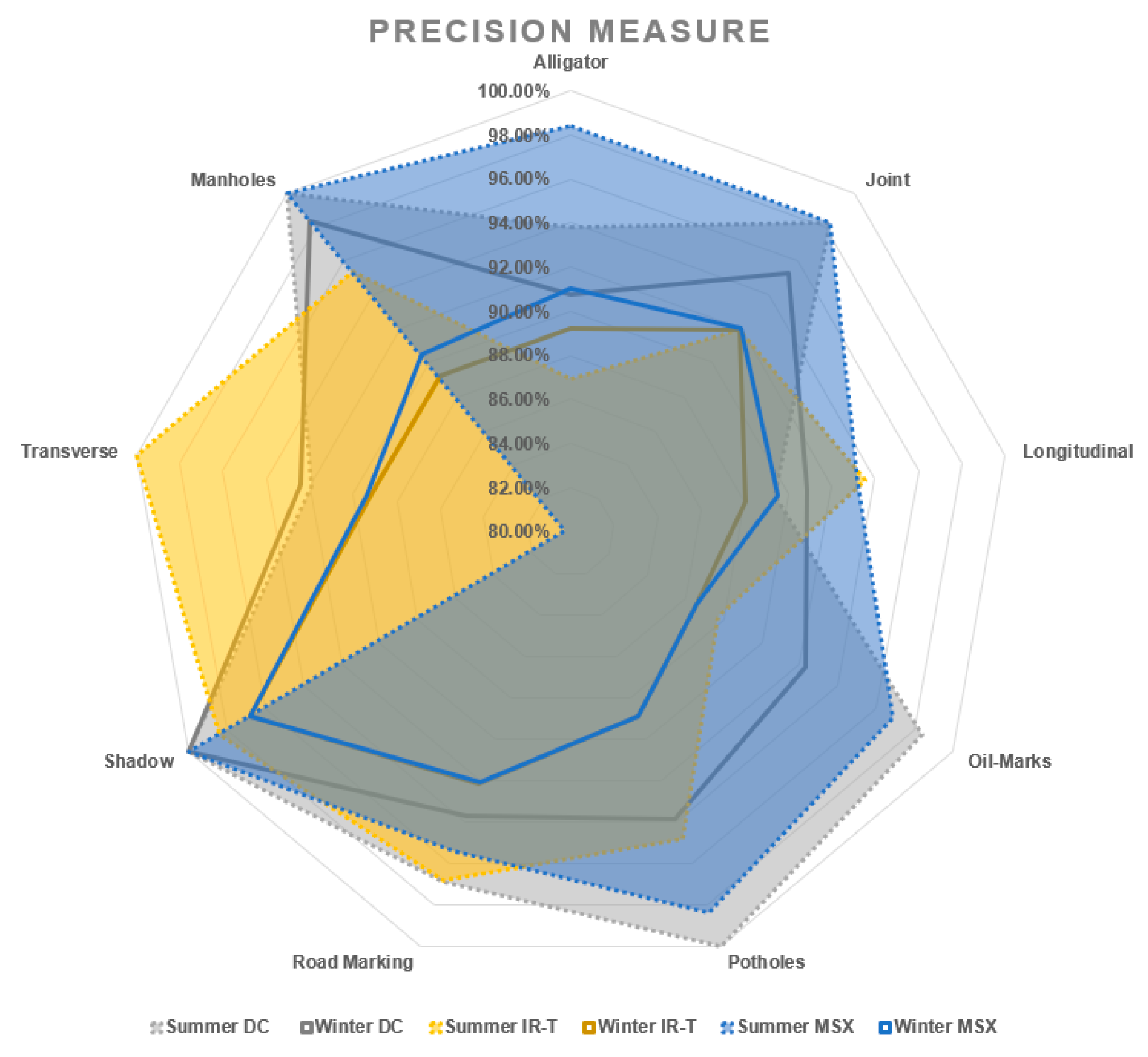
- The data captured in sunny conditions during summer and winter show a prediction accuracy of DC = 96.47% > MSX = 95.24% > IR-T = 93.83% and DC = 94.14% > MSX = 90.69% > IR-T = 90.173%, respectively.
- From DC image input, the sensitivity was 96.47% for summer conditions and 94.20% for winter conditions. With the capturing method being manual, the deep learning technique can categorise pavement features reliably irrespective of the weather season.
- From IR-T and MSX image input, over 90% precision (93.95% summer IR-T, 90.23% for winter conditions IR-T, 95.65% for summer MSX and 90.76% for winter MSX) suggests that the prevalence of the temperature profile in pavement features can be gainfully utilised to categorise them irrespective of the weather season.
- With summer conditions showing better overall prediction accuracy than winter conditions, we suggest that an inexpensive IR-T imaging camera with a medium resolution level can still be economical, unlike expensive alternate options; however, its usage is limited to summer sunny conditions.
Author Contributions
Funding
Institutional Review Board Statement
Informed Consent Statement
Data Availability Statement
Conflicts of Interest
References
- Chen, C.; Seo, H.; Jun, C.H.; Zhao, Y. Pavement crack detection and classification based on fusion feature of LBP and PCA with SVM. Int. J. Pavement Eng. 2021, 23, 3274–3283. [Google Scholar] [CrossRef]
- Kamdi, S.; Krishna, R.K. Image Segmentation and region growing algorithm. Int. J. Comput. Technol. Electron. Eng. 2012, 2, 103–107. [Google Scholar]
- Shrivakshan, G.T.; Chandrasekar, C. A Comparison of various Edge Detection Techniques used in Image Processing. Int. J. Comput. Sci. 2012, 9, 269–276. [Google Scholar]
- Kang, C.L.; Wang, F.; Zong, M.M.; Cheng, Y.; Lu, T.N. Research on Improved Region Growing Point Cloud Algorithm. ISPRS Int. Arch. Photogramm. Remote Sens. Spat. Inf. Sci. 2020, XLII-3/W10, 153–157. [Google Scholar] [CrossRef]
- Cao, W.; Liu, Q.; He, Z. Review of Pavement Defect Detection Methods. IEEE Access 2020, 8, 14531–14544. [Google Scholar] [CrossRef]
- Hou, Y.; Li, Q.; Zhang, C.; Lu, G.; Ye, Z.; Chen, Y.; Wang, L.; Cao, D. The State-of-the-Art Review on Applications of Intrusive Sensing, Image Processing Techniques, and Machine Learning Methods in Pavement Monitoring and Analysis. Engineering 2020, 7, 845–856. [Google Scholar] [CrossRef]
- Yusof, N.A.M.; Ibrahim, A.; Noor, M.H.M.; Tahir, N.M.; Abidin, N.Z.; Osman, M.K. Deep convolution neural network for crack detection on asphalt pavement. J. Phys. Conf. Ser. 2019, 1349, 012020. [Google Scholar] [CrossRef]
- Cha, Y.-J.; Choi, W.; Büyüköztürk, O. Deep Learning-Based Crack Damage Detection Using Convolutional Neural Networks. Comput. Civ. Infrastruct. Eng. 2017, 32, 361–378. [Google Scholar] [CrossRef]
- Gopalakrishnan, K.; Khaitan, S.K.; Choudhary, A.; Agrawal, A. Deep Convolutional Neural Networks with transfer learning for computer vision-based data-driven pavement distress detection. Constr. Build. Mater. 2017, 157, 322–330. [Google Scholar] [CrossRef]
- Zhang, K.; Cheng, H.-D.; Gai, S. Efficient Dense-Dilation Network for Pavement Cracks Detection with Large Input Image Size. In Proceedings of the 21st International Conference on Intelligent Transportation Systems (ITSC), Maui, HI, USA, 4–7 November 2018; pp. 884–889. [Google Scholar]
- Majidifard, H.; Adu-Gyamfi, Y.; Buttlar, W.G. Deep machine learning approach to develop a new asphalt pavement condition index. Constr. Build. Mater. 2020, 247, 118513. [Google Scholar] [CrossRef]
- Chen, C.; Seo, H.; Zhao, Y. A novel pavement transverse cracks detection model using WT-CNN and STFT-CNN for smartphone data analysis. Int. J. Pavement Eng. 2021, 23, 4372–4384. [Google Scholar] [CrossRef]
- Chen, C.; Seo, H.; Jun, C.; Zhao, Y. A potential crack region method to detect crack using image processing of multiple thresholding. Signal Image Video Process. 2022, 16, 1673–1681. [Google Scholar] [CrossRef]
- Zhu, J.; Song, J. Weakly supervised network based intelligent identification of cracks in asphalt concrete bridge deck. Alex. Eng. J. 2020, 59, 1307–1317. [Google Scholar] [CrossRef]
- Guan, J.; Yang, X.; Ding, L.; Cheng, X.; Lee, V.C.; Jin, C. Automated pixel-level pavement distress detection based on stereo vision and deep learning. Autom. Constr. 2021, 129, 103788. [Google Scholar] [CrossRef]
- Szegedy, C.; Liu, W.; Jia, Y.; Sermanet, P.; Reed, S.; Anguelov, D.; Rabinovich, A. Going deeper with convolutions. In Proceedings of the IEEE Conference on Computer Vision and Pattern Recognition, Boston, MA, USA, 7–12 June 2015; pp. 1–9. [Google Scholar]
- Zheng, Q.; Yang, M.; Yang, J.; Zhang, Q.; Zhang, X. Improvement of generalization ability of deep CNN via implicit regularization in two-stage training process. IEEE Access 2018, 6, 15844–15869. [Google Scholar] [CrossRef]
- Seo, H. Infrared thermography for detecting cracks in pillar models with different reinforcing systems. Tunn. Undergr. Space Technol. 2021, 116, 104118. [Google Scholar] [CrossRef]
- Seo, H.; Choi, H.; Park, J.; Lee, I.-M. Crack detection in pillars using infrared thermographic imaging. Geotech. Test. J. 2017, 40, 371–380. [Google Scholar] [CrossRef]
- Seo, H.; Zhao, Y.; Chen, C. Displacement Mapping of Point Clouds for Retaining Structure Considering Shape of Sheet Pile and Soil Fall Effects during Excavation. J. Geotech. Geoenviron. Eng. 2022, 148, 04022016. [Google Scholar] [CrossRef]
- Seo, H. Long-term Monitoring of zigzag-shaped concrete panel in retaining structure using laser scanning and analysis of influencing factors. Opt. Lasers Eng. 2021, 139, 106498. [Google Scholar] [CrossRef]
- Seo, H. Monitoring of CFA pile test using three dimensional laser scanning and distributed fiber optic sensors. Opt. Lasers Eng. 2020, 130, 106089. [Google Scholar] [CrossRef]
- Seo, H. 3D roughness measurement of failure surface in CFA pile samples using three-dimensional laser scanning. Appl. Sci. 2021, 11, 2713. [Google Scholar] [CrossRef]
- Zhao, Y.; Seo, H.; Chen, C. Displacement analysis of point cloud removed ground collapse effect in SMW by CANUPO machine learning algorithm. J. Civ. Struct. Health Monit. 2022, 12, 447–463. [Google Scholar] [CrossRef]
- Chen, C.; Chandra, S.; Han, Y.; Seo, H. Deep Learning-Based Thermal Image Analysis for Pavement Defect Detection and Classification Considering Complex Pavement Conditions. Remote Sens. 2021, 14, 106. [Google Scholar] [CrossRef]
- Chen, C.; Chandra, S.; Seo, H. Automatic Pavement Defect Detection and Classification Using RGB-Thermal Images Based on Hierarchical Residual Attention Network. Sensors 2022, 22, 5781. [Google Scholar] [CrossRef] [PubMed]
- Huang, Y.; Li, Y.; Zhang, Y. A Retinex Image Enhancement based on L Channel Illumination Estimation and Gamma Function. In Proceedings of the 2018 Joint International Advanced Engineering and Technology Research Conference, Xi’an, China, 26–27 May 2018; pp. 312–317. [Google Scholar]
- Jin, B.; Cruz, L.; Goncalves, N. Pseudo RGB-D Face Recognition. IEEE Sens. J. 2022, 22, 21780–21794. [Google Scholar] [CrossRef]
- PyTorch, 2020. PyTorch Tutorials. Available online: https://pytorch.org/tutorials/beginner/nlp/deep_learning_tutorial.html#creating-network-components-in-pytorch (accessed on 20 August 2021).
- Zhang, Q.L.; Yang, Y.B. SA-NET: Shuffle attention for deep convolutional Neural Networks. In Proceedings of the IEEE International Conference on Acoustics, Speech and Signal Processing, Virtual, 6–12 June 2021; pp. 2235–2239. [Google Scholar]
- Zhao, M.; Jha, A.; Liu, Q.; Millis, B.A.; Mahadevan-Jansen, A.; Lu, L.; Landman, B.A.; Tyska, M.J.; Huo, Y. Faster Mean-shift: GPU-accelerated clustering for cosine embedding-based cell segmentation and tracking. Med Image Anal. 2021, 71, 102048. [Google Scholar] [CrossRef]
- Zhao, M.; Liu, Q.; Jha, A.; Deng, R.; Yao, T.; Mahadevan-Jansen, A.; Tyska, M.J.; Millis, B.A.; Huo, Y. VoxelEmbed: 3D instance segmentation and tracking with voxel embedding based deep learning. In International Workshop on Machine Learning in Medical Imaging; Springer: Cham, Switzerland, 2021; pp. 437–446. [Google Scholar]


| Deep Learning Algorithm Parameters | Parameter Details |
|---|---|
| Dataset considerations | Every 8th image identified as evaluation image |
| Evaluation = 567 DC + 567 IR + 567 MSX images | |
| Training = 3933 DC + 3933 IR + 3933 MSX images | |
| Functional parameter | Cross-entropy loss function |
| Stochastic paddle optimiser | |
| Model parameters | Hyperparameter-tuned learning rate |
| 0.9 momentum | |
| 100 epoch times | |
| Batch size 48 |
| Layer (Type) | Output Shape | Parameter |
|---|---|---|
| Input layer | [(None, 256, 256, 3)] | 0 |
| Functional | (None, 8, 8, 512) | 14,714,688 |
| Global average pooling | (None, 512) | 0 |
| Dense | (None, 1024) | 525,312 |
| Additional dense | (None, 8) | 8200 |
| Total parameters: 15,248,200 | ||
| Trainable parameters: 533,512 | ||
| Non-trainable parameters: 14,714,688 | ||
| Total | Train (60%) | Validation (20%) | Test (20%) | |
|---|---|---|---|---|
| Original dataset | 13,500 | 8100 | 2700 | 2700 |
| Augmented dataset | 18,945 | 11,367 | 3789 | 3789 |
| Actual (Summer Conditions) | Precision | ||||
|---|---|---|---|---|---|
| Alligator Cracks | Other Categories | Total | |||
| Predicted | Alligator cracks | 61 | 4 | 65 | 61/65 = 93.85% |
| Other categories | 2 | 500 | 502 | ||
| Total | 63 | 504 | 567 | ||
| Sensitivity | 61/63 = 96.83% | 561/561 = 98.94% | |||
| Summer Sunny Condition | Winter Sunny Condition | |||||
|---|---|---|---|---|---|---|
| Accuracy | Precision | Recall | Accuracy | Precision | Recall | |
| DC | 96.57% | 96.59% | 96.57% | 94.14% | 92.19% | 92.20% |
| IR-T | 93.83% | 93.95% | 93.83% | 90.17% | 90.23% | 90.63% |
| MSX | 96.83% | 96.92% | 96.83% | 90.69% | 90.76% | 91.15% |
| Summer Sunny Conditions | Winter Sunny Conditions | |||||
|---|---|---|---|---|---|---|
| DC | IR-T | MSX | DC | IR-T | MSX | |
| Alligator | 96.83% | 95.24% | 96.83% | 90.77% | 90.63% | 90.91% |
| Joint | 93.65% | 90.48% | 90.48% | 91.04% | 89.06% | 89.23% |
| Longitudinal | 93.65% | 92.06% | 87.30% | 90.91% | 88.06% | 89.55% |
| Oil marking | 98.41% | 90.48% | 98.41% | 96.77% | 82.86% | 84.06% |
| Pothole | 95.24% | 87.30% | 95.24% | 92.42% | 90.32% | 91.80% |
| Road marking | 100% | 96.83% | 100% | 95.24% | 92.19% | 92.06% |
| Shadow | 100% | 98.41% | 98.41% | 100% | 98.36% | 96.77% |
| Transverse | 90.48% | 95.24% | 96.93% | 95.31% | 93.55% | 89.39% |
| Manholes | 100% | 98.41% | 93.65% | 95.38% | 90.63% | 90.48% |
| Average | 96.47% | 93.83% | 95.24% | 94.20% | 90.17% | 90.76% |
Publisher’s Note: MDPI stays neutral with regard to jurisdictional claims in published maps and institutional affiliations. |
© 2022 by the authors. Licensee MDPI, Basel, Switzerland. This article is an open access article distributed under the terms and conditions of the Creative Commons Attribution (CC BY) license (https://creativecommons.org/licenses/by/4.0/).
Share and Cite
Chandra, S.; AlMansoor, K.; Chen, C.; Shi, Y.; Seo, H. Deep Learning Based Infrared Thermal Image Analysis of Complex Pavement Defect Conditions Considering Seasonal Effect. Sensors 2022, 22, 9365. https://doi.org/10.3390/s22239365
Chandra S, AlMansoor K, Chen C, Shi Y, Seo H. Deep Learning Based Infrared Thermal Image Analysis of Complex Pavement Defect Conditions Considering Seasonal Effect. Sensors. 2022; 22(23):9365. https://doi.org/10.3390/s22239365
Chicago/Turabian StyleChandra, Sindhu, Khaled AlMansoor, Cheng Chen, Yunfan Shi, and Hyungjoon Seo. 2022. "Deep Learning Based Infrared Thermal Image Analysis of Complex Pavement Defect Conditions Considering Seasonal Effect" Sensors 22, no. 23: 9365. https://doi.org/10.3390/s22239365
APA StyleChandra, S., AlMansoor, K., Chen, C., Shi, Y., & Seo, H. (2022). Deep Learning Based Infrared Thermal Image Analysis of Complex Pavement Defect Conditions Considering Seasonal Effect. Sensors, 22(23), 9365. https://doi.org/10.3390/s22239365