
Algorithm to Correct Measurement Offsets Introduced by Inactive Elements of Transducer Arrays in Ultrasonic Flow Metering

 , , , , and
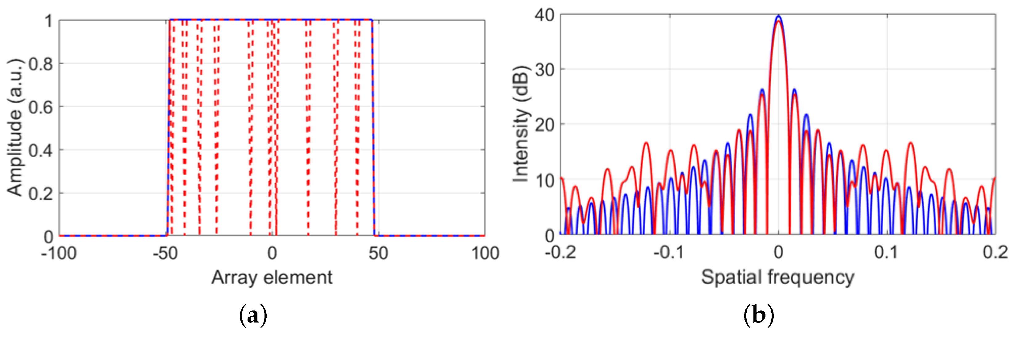
Abstract
1. Introduction
2. Measurement Offsets Introduced by Inactive Transducer Array Elements
2.1. On the Shape of the Beam
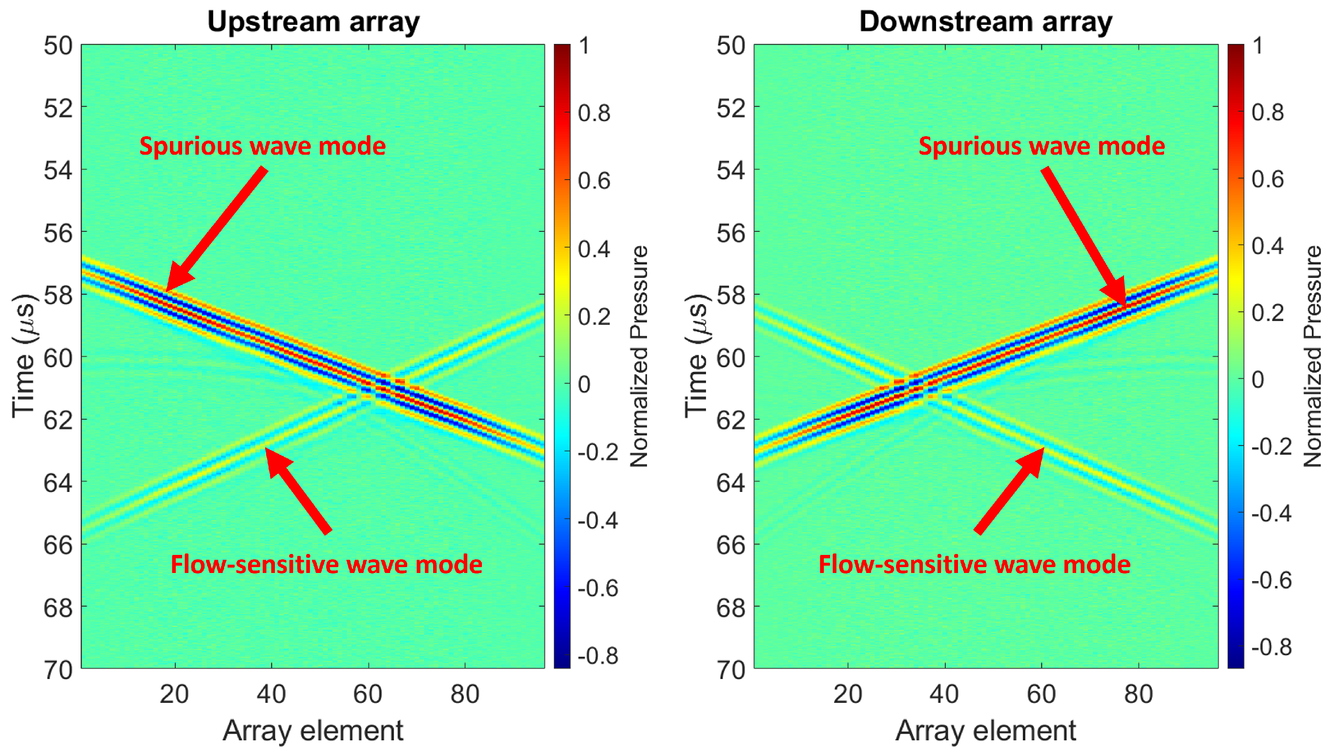
2.2. On the Travel Path
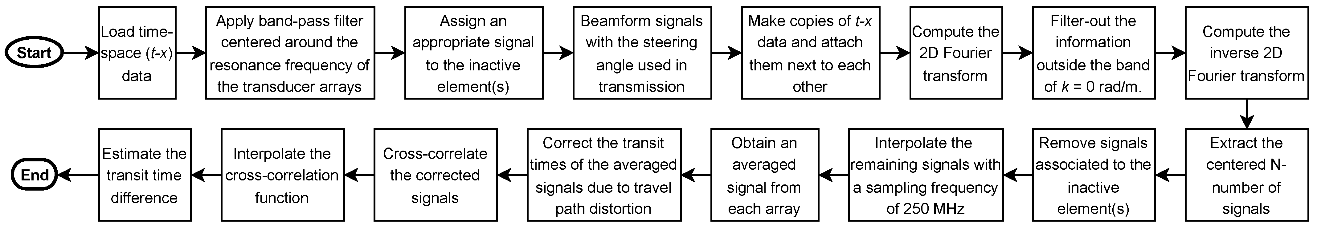
3. Algorithm
4. Validation of the Algorithm
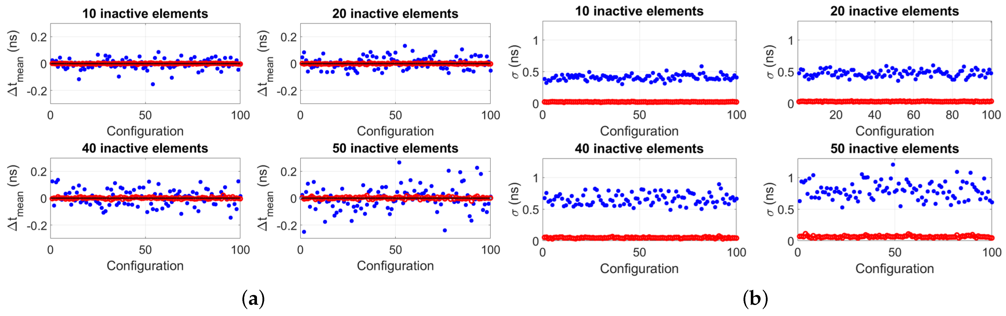
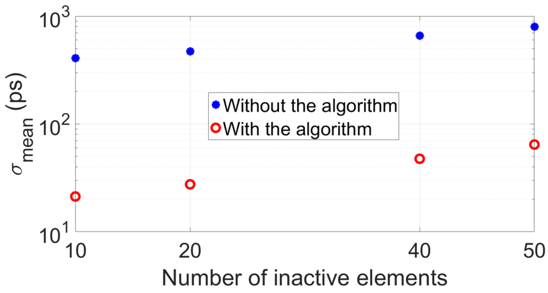
4.1. Simulation
4.1.1. Settings
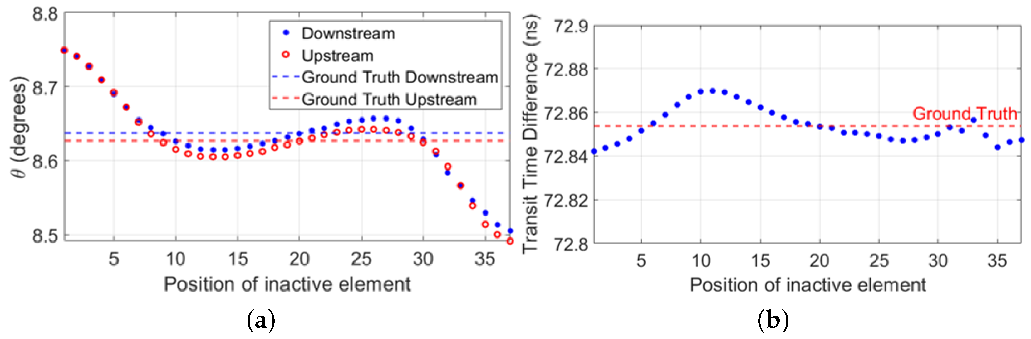
4.1.2. Results
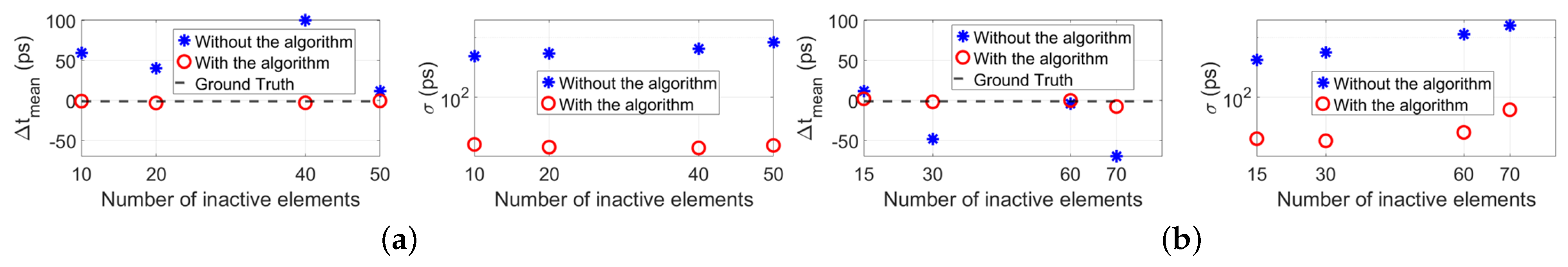
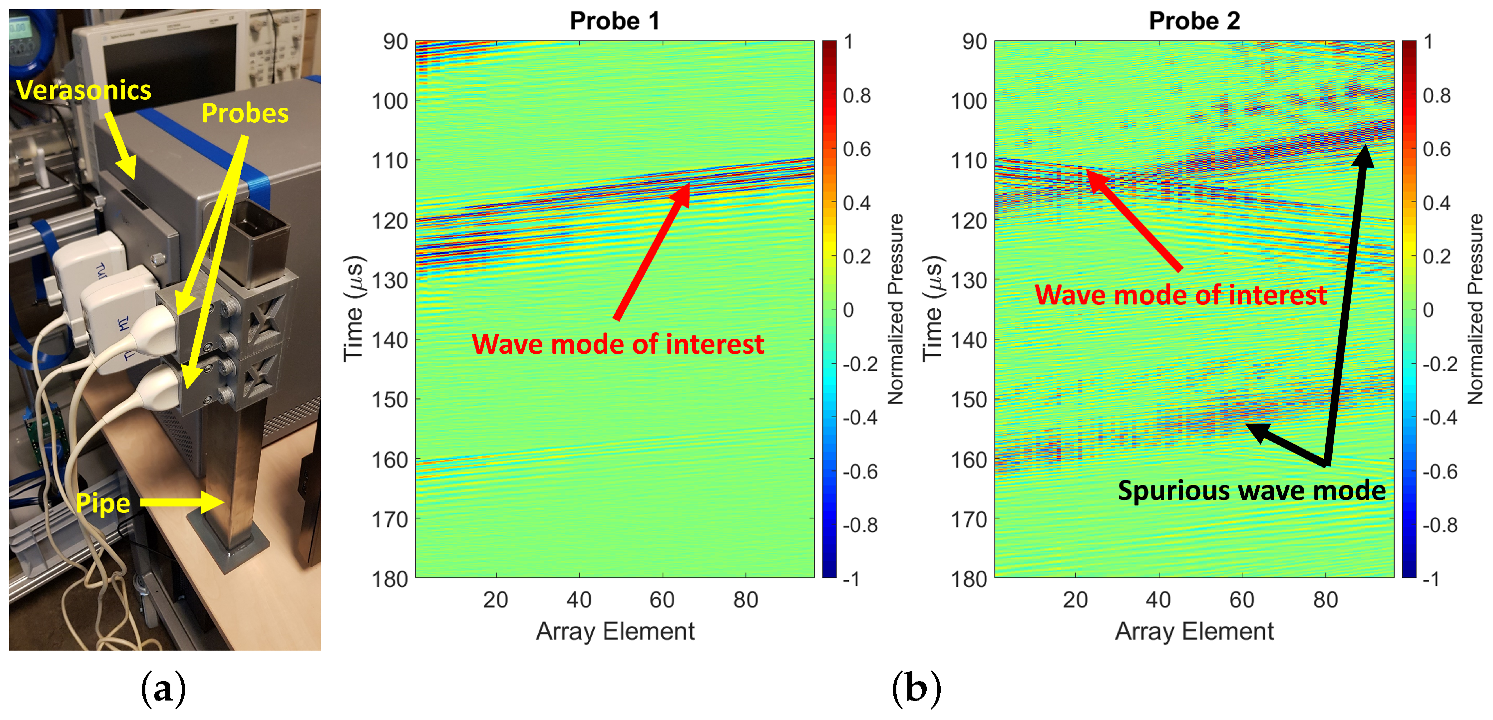
4.2. Experiment
4.2.1. Setup
4.2.2. Results
5. Discussion
6. Conclusions
Author Contributions
Funding
Institutional Review Board Statement
Informed Consent Statement
Data Availability Statement
Conflicts of Interest
Abbreviations
| UFMs | Ultrasonic flow meters |
| SNR | Signal-to-noise ratio |
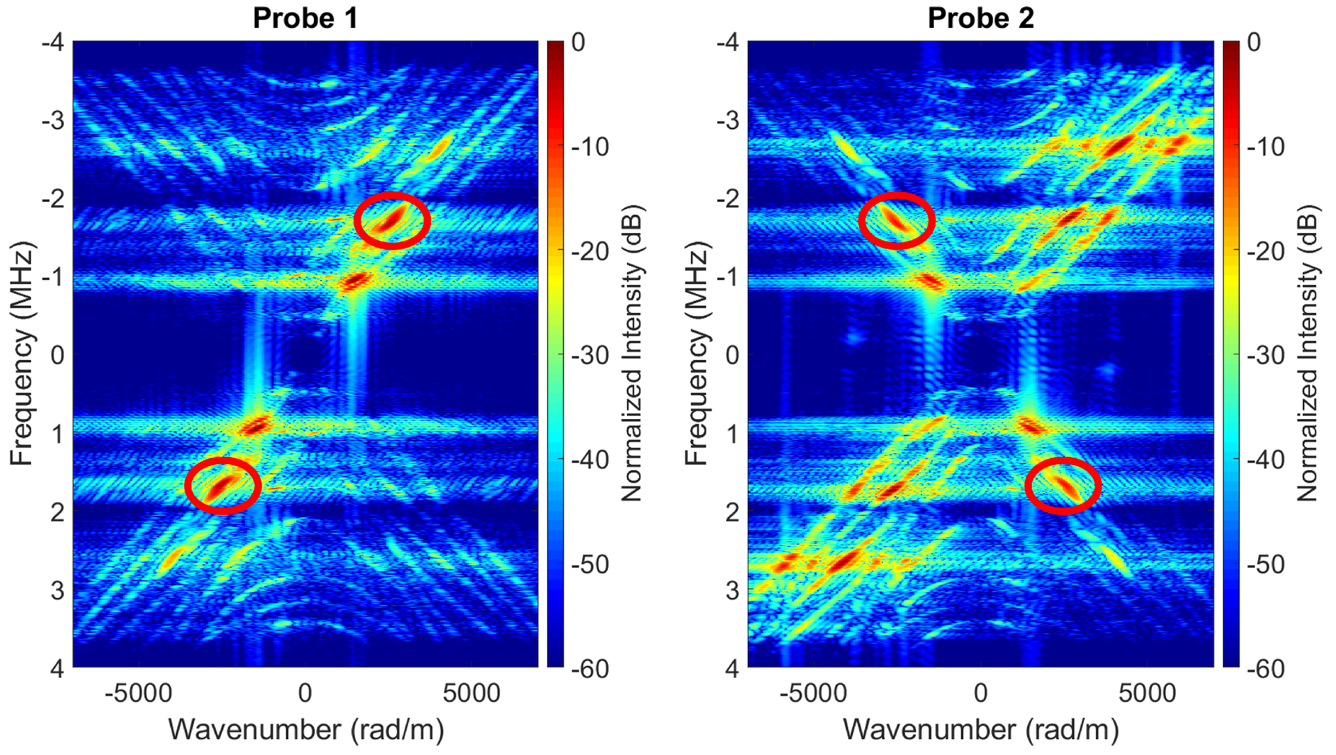
| t-x | time-space |
| f-kx | frequency-wavenumber |
References
- Baker, R.C. Flow Measurement Handbook: Industrial Designs, Operating Principles, Performance, and Applications; Cambridge University Press: Cambridge, UK, 2005. [Google Scholar]
- Kang, L.; Feeney, A.; Su, R.; Lines, D.; Ramadas, S.N.; Rowlands, G.; Dixon, S. Flow velocity measurement using a spatial averaging method with two-dimensional flexural ultrasonic array technology. Sensors 2019, 19, 4786. [Google Scholar] [CrossRef] [PubMed]
- Wendoloski, J.C. On the theory of acoustic flow measurement. J. Acoust. Soc. Am. 2001, 110, 724–737. [Google Scholar] [CrossRef]
- Lynnworth, L.C. Ultrasonic Measurements for Process Control: Theory, Techniques, Applications; Academic Press: Cambridge, MA, USA, 2013. [Google Scholar]
- Massaad, J.; van Neer, P.L.M.J.; van Willigen, D.M.; de Jong, N.; Pertijs, M.A.; Verweij, M.D. Exploiting nonlinear wave propagation to improve the precision of ultrasonic flow meters. Ultrasonics 2021, 116, 106476. [Google Scholar] [CrossRef] [PubMed]
- Clay, A.C.; Wooh, S.C.; Azar, L.; Wang, J.Y. Experimental study of phased array beam steering characteristics. J. Nondestruct. Eval. 1999, 18, 59–71. [Google Scholar] [CrossRef]
- Dai, Y.X.; Yan, S.G.; Zhang, B.X. Ultrosonic beam steering behavior of linear phased arrays in solid. In Proceedings of the 2019 14th Symposium on Piezoelectrcity, Acoustic Waves and Device Applications (SPAWDA), Shijiazhuang, China, 1–4 November 2019; pp. 1–5. [Google Scholar]
- Massaad, J.; van Neer, P.L.M.J.; van Willigen, D.M.; Pertijs, M.A.; de Jong, N.; Verweij, M.D. Measurement of Pipe and Liquid Parameters Using the Beam Steering Capabilities of Array-Based Clamp-On Ultrasonic Flow Meters. Sensors 2022, 22, 5068. [Google Scholar] [CrossRef] [PubMed]
- Massaad, J.; Van Neer, P.L.M.J.; Van Willigen, D.M.; Noothout, E.C.; De Jong, N.; Pertijs, M.A.; Verweij, M.D. Design and Proof-of-Concept of a Matrix Transducer Array for Clamp-On Ultrasonic Flow Measurements. IEEE Trans. Ultrason. Ferroelectr. Freq. Control 2022, 69, 2555–2568. [Google Scholar] [CrossRef] [PubMed]
- Lee, Y.C.; Cheng, S.W. Measuring Lamb wave dispersion curves of a bi-layered plate and its application on material characterization of coating. IEEE Trans. Ultrason. Ferroelectr. Freq. Control 2001, 48, 830–837. [Google Scholar] [PubMed]
- Bernal, M.; Nenadic, I.; Urban, M.W.; Greenleaf, J.F. Material property estimation for tubes and arteries using ultrasound radiation force and analysis of propagating modes. J. Acoust. Soc. Am. 2011, 129, 1344–1354. [Google Scholar] [CrossRef]
- Foiret, J.; Minonzio, J.G.; Chappard, C.; Talmant, M.; Laugier, P. Combined estimation of thickness and velocities using ultrasound guided waves: A pioneering study on in vitro cortical bone samples. IEEE Trans. Ultrason. Ferroelectr. Freq. Control 2014, 61, 1478–1488. [Google Scholar] [CrossRef]
- Chillara, V.K.; Sturtevant, B.T.; Pantea, C.; Sinha, D.N. Ultrasonic sensing for noninvasive characterization of oil-water-gas flow in a pipe. In Proceedings of the AIP Conference Proceedings; AIP Publishing LLC: Atlanta, GA, USA, 2017; Volume 1806, p. 090014. [Google Scholar]
- Chillara, V.K.; Sturtevant, B.; Pantea, C.; Sinha, D.N. A Physics-Based Signal Processing Approach for Noninvasive Ultrasonic Characterization of Multiphase Oil–Water–Gas Flows in a Pipe. IEEE Trans. Ultrason. Ferroelectr. Freq. Control 2020, 68, 1328–1346. [Google Scholar] [CrossRef]
- Greenhall, J.; Hakoda, C.; Davis, E.S.; Chillara, V.K.; Pantea, C. Noninvasive acoustic measurements in cylindrical shell containers. IEEE Trans. Ultrason. Ferroelectr. Freq. Control 2021, 68, 2251–2258. [Google Scholar] [CrossRef] [PubMed]
- Massaad, J.; Van Neer, P.L.M.J.; Van Willigen, D.M.; Sabbadini, A.; De Jong, N.; Pertijs, M.A.; Verweij, M.D. Measurement of Pipe and Fluid Properties With a Matrix Array-Based Ultrasonic Clamp-On Flow Meter. IEEE Trans. Ultrason. Ferroelectr. Freq. Control 2021, 69, 309–322. [Google Scholar] [CrossRef] [PubMed]
- Massaad, J.; van Neer, P.L.M.J.; van Willigen, D.M.; Pertijs, M.A.; de Jong, N.; Verweij, M.D. Suppression of Lamb wave excitation via aperture control of a transducer array for ultrasonic clamp-on flow metering. J. Acoust. Soc. Am. 2020, 147, 2670–2681. [Google Scholar] [CrossRef] [PubMed]
- Alleyne, D.; Cawley, P. A two-dimensional Fourier transform method for the measurement of propagating multimode signals. J. Acoust. Soc. Am. 1991, 89, 1159–1168. [Google Scholar] [CrossRef]
- Weigang, B.; Moore, G.W.; Gessert, J.; Phillips, W.H.; Schafer, M. The methods and effects of transducer degradation on image quality and the clinical efficacy of diagnostic sonography. J. Diagn. Med. Sonogr. 2003, 19, 3–13. [Google Scholar] [CrossRef]
- Vachutka, J.; Dolezal, L.; Kollmann, C.; Klein, J. The effect of dead elements on the accuracy of Doppler ultrasound measurements. Ultrason. Imaging 2014, 36, 18–34. [Google Scholar] [CrossRef]
- Welsh, D.; Inglis, S.; Pye, S.D. Detecting failed elements on phased array ultrasound transducers using the Edinburgh Pipe Phantom. Ultrasound 2016, 24, 68–93. [Google Scholar] [CrossRef]
- Cobbold, R.S. Foundations of Biomedical Ultrasound; Oxford University Press: Oxford, UK, 2006. [Google Scholar]
- Spitz, S. Seismic trace interpolation in the FX domain. Geophysics 1991, 56, 785–794. [Google Scholar] [CrossRef]
- Gülünay, N. Seismic trace interpolation in the Fourier transform domain. Geophysics 2003, 68, 355–369. [Google Scholar] [CrossRef]
- Naghizadeh, M.; Sacchi, M.D. f-x adaptive seismic-trace interpolation. Geophysics 2009, 74, V9–V16. [Google Scholar] [CrossRef]
- van den Berg, E.; Friedlander, M.P. SPOT-A linear operator toolbox for Matlab. 2013. Available online: https://www.cs.ubc.ca/labs/scl/spot/ (accessed on 2 November 2022).
- Wang, Y.; Wang, B.; Tu, N.; Geng, J. Seismic trace interpolation for irregularly spatial sampled data using convolutional autoencoder. Geophysics 2020, 85, V119–V130. [Google Scholar] [CrossRef]
- Jensen, J.A.; Svendsen, N.B. Calculation of pressure fields from arbitrarily shaped, apodized, and excited ultrasound transducers. IEEE Trans. Ultrason. Ferroelectr. Freq. Control 1992, 39, 262–267. [Google Scholar] [CrossRef] [PubMed]
- Jensen, J.A. Field: A program for simulating ultrasound systems. In Proceedings of the 10th Nordic-Baltic Conference on Biomedical Imaging, Tampere, Finland, 9 June 1996; Volume 4. Supplement 1, Part 1: 351–353. [Google Scholar]


Publisher’s Note: MDPI stays neutral with regard to jurisdictional claims in published maps and institutional affiliations. |
© 2022 by the authors. Licensee MDPI, Basel, Switzerland. This article is an open access article distributed under the terms and conditions of the Creative Commons Attribution (CC BY) license (https://creativecommons.org/licenses/by/4.0/).
Share and Cite
Massaad, J.; van Neer, P.L.M.J.; van Willigen, D.M.; Pertijs, M.A.P.; de Jong, N.; Verweij, M.D. Algorithm to Correct Measurement Offsets Introduced by Inactive Elements of Transducer Arrays in Ultrasonic Flow Metering. Sensors 2022, 22, 9317. https://doi.org/10.3390/s22239317
Massaad J, van Neer PLMJ, van Willigen DM, Pertijs MAP, de Jong N, Verweij MD. Algorithm to Correct Measurement Offsets Introduced by Inactive Elements of Transducer Arrays in Ultrasonic Flow Metering. Sensors. 2022; 22(23):9317. https://doi.org/10.3390/s22239317
Chicago/Turabian StyleMassaad, Jack, Paul L. M. J. van Neer, Douwe M. van Willigen, Michiel A. P. Pertijs, Nicolaas de Jong, and Martin D. Verweij. 2022. "Algorithm to Correct Measurement Offsets Introduced by Inactive Elements of Transducer Arrays in Ultrasonic Flow Metering" Sensors 22, no. 23: 9317. https://doi.org/10.3390/s22239317
APA StyleMassaad, J., van Neer, P. L. M. J., van Willigen, D. M., Pertijs, M. A. P., de Jong, N., & Verweij, M. D. (2022). Algorithm to Correct Measurement Offsets Introduced by Inactive Elements of Transducer Arrays in Ultrasonic Flow Metering. Sensors, 22(23), 9317. https://doi.org/10.3390/s22239317