
Real-Time Vehicle Classification System Using a Single Magnetometer


Abstract
1. Introduction
2. Related Work and Contributions
2.1. Vehicle Detection Using Magnetic Sensors
2.2. Vehicle Classification Using Magnetic Sensors
2.3. Motivation and Contributions
- In this study, nine vehicle classes were defined and utilized to explore the capabilities of the magnetometer-based technology. This number is much higher compared to relevant methods, where, as described in Section 2.2, vehicles were classified into two to five classes.
- Drawbacks of reported studies are, that most works applied only a small number of collected samples, and many do not consider unknown data to validate their developed algorithms. In this work, a very high number of samples were used to construct training and validation datasets.
- Related works mainly do not deal with the implementation of the algorithms. In the proposed system, all parts of the vehicle classification algorithm are realized on the used microcontroller-based hardware. To achieve online and real-time operation, the feature set consists of only time-domain features, which require less computation and memory resources than necessary for frequency-domain analysis, which were also widely used in other studies.
- Different novel feature extraction modes are proposed to minimize the number of used features and the possible cost of the system. Various combinations of applied sensor axes were also compared using the proposed feature set to find the optimal setup.
- Other disadvantages of many works include the utilization of the length of the detection as one of the inputs in the classification stage. This feature provides valuable information about the length of the vehicle, but it obviously has a negative effect on recognition efficiency if the unit is placed in a location where the speed is different to the location where the training samples were collected. The effect of this feature in the proposed system was also investigated to explore the suitability of the applied feature set.
3. Measurement
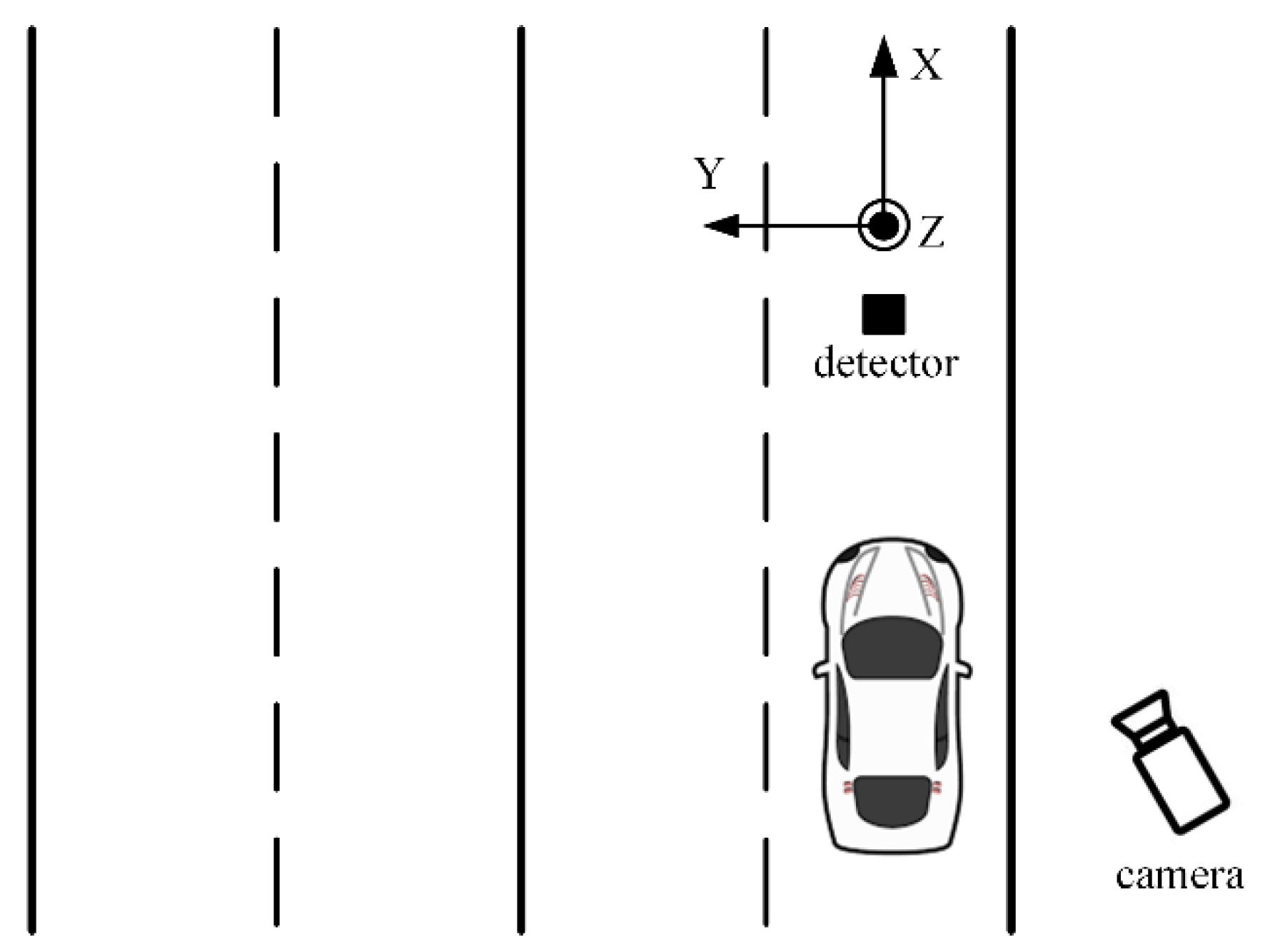
3.1. Measurement Unit
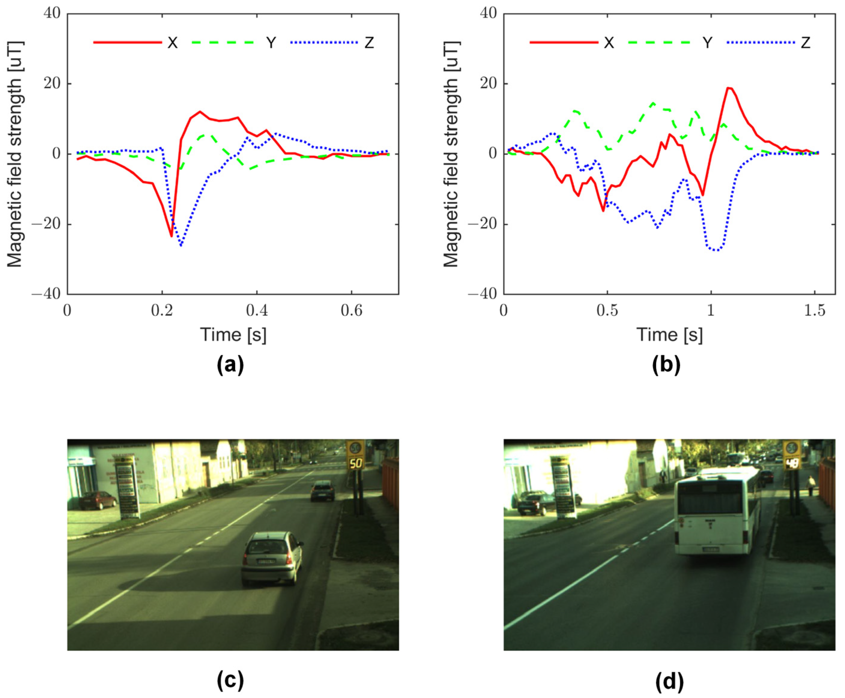
3.2. Data Acquisition
4. Vehicle Classification Algorithm
4.1. Vehicle Detection Algorithm
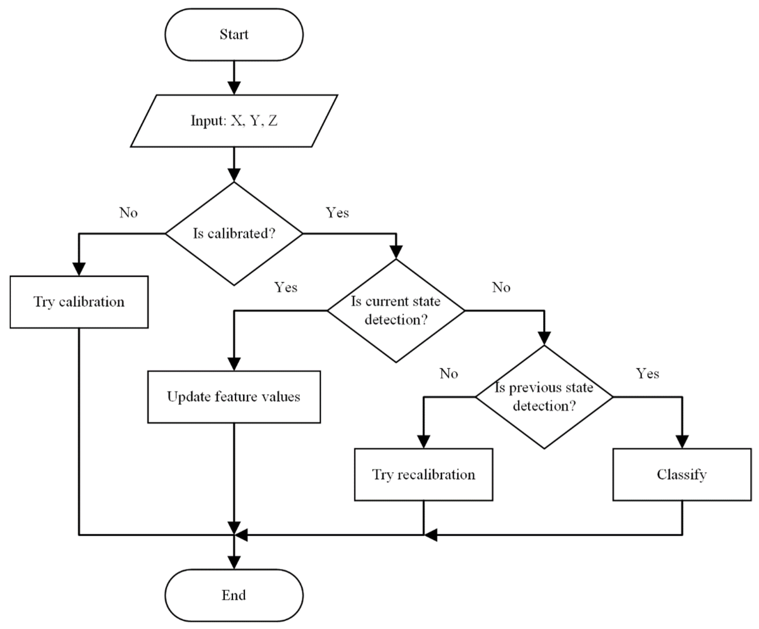
- When the unit is turned on, the calibration process is run. This process uses a calibration range size, which must be slightly larger than the peak-to-peak noise level, because it should follow the slow changes in the environment. This noise level should be estimated after the installation of the unit in the current location, when no vehicles are near to the sensor. During calibration, the highest and lowest measurement values are monitored in a measurement window for all three axes. The difference between the highest and lowest values must be smaller than the calibration range size. The calibration is restarted if the difference exceeds the range size at any time in the window at any of the axes. This filters the factors which affect the magnetic field near the sensor. The size of the measurement window should be at least 1 s based on experience. If the calibration is successful, the upper and lower calibration and detection thresholds are calculated for all axes. This is done by equally stretching the range determined by the highest and lowest values to the width defined by the range sizes.
- Vehicle presence is declared if the measurement values exceed the detection threshold at both X and Z axes.
- The detection flag is cleared if the measurement values on both X and Z axes are between the calibration thresholds for a previously defined number of measurements. The algorithm should be suitable for detecting vehicles with trailers, so the used length should be calculated using the potential speed on the location and the possible distance between the vehicle and the trailer.
- A recalibration is attempted always when vehicle presence is not declared. The process is the same as during calibration, but the measured highest and lowest measurements must fit into the previous calibration range. This enables the following of the environmental changes.
4.2. Feature Extraction
4.2.1. Feature Types
- Detection length (DL): The number of measurements in the detection window.
- Highest value (MAX) and lowest value (MIN): The highest and lowest measurement values in the detection window.
- Place of the highest and lowest values (PlaceMax, PlaceMin): The indexes of the measurements where the MAX and MIN points were found, both divided with the detection length.
- Range changes (RCH): The calibration thresholds define three ranges in the signal values, one above the upper threshold, one under the lower, and one between them. This feature measures how many times has the signal switched ranges.
- Number of local maxima and minima (NumLocMax, NumLocMin): The number of local maxima in the range above the upper threshold, and the number of local minima in the range under the lower threshold. A point is considered as a local maximum (minimum) if it has local minima (maxima) before and after it, and the differences in the amplitude are higher than the peak-to-peak noise value.
- Mean absolute value (MAV): The mean absolute amplitude value, which can be calculated aswhere N is the number of samples in the detection window and xi are the signal amplitudes at the given index.
- Mean value (MV): The mean amplitude value.
- Number of slope sign changes (NSSC): The number of direction changes, where among the three consecutive values the first or the last changes are larger than a predefined th threshold, which is the peak-to-peak noise level (2).
- Number of zero crossings (NZC): The number of times when the amplitude values cross the zero-amplitude level and the difference between the values with opposite signs is larger than the threshold:
- Average waveform length (AWL): The length of the waveform over the detection window divided by the number of samples in the window:
- Root mean square (RMS): The calculation of the RMS can be performed as given in (5).
- Willison amplitude (WAMP): The number of amplitude changes in the window, which are higher than the given threshold level (6).
4.2.2. Extraction Modes
- Measurement axes (X, Y, Z): The features were computed using the raw measurement values on each axis. The calibrated offsets were subtracted from the measured values.
- Absolute values (Xabs, Yabs, Zabs): The computed absolute values were applied on each measurement axis, which were calculated after the offsets were subtracted from the measurement values.
- Magnitude from the origin (XYO, XZO, YZO, XYZO): Magnitude values were computed in three dimensions and in two dimensions using different combination of the axes. The magnitude of the calibration point was subtracted from computed magnitudes. These data provide information about the changes in magnitude in different planes and in 3D based on the sensor frame compared to the magnitudes given by the calibration point.where Xcal, Ycal, and Zcal define the calibration point, which are the middle points between the upper and lower calibration thresholds on each sensor axis.
- Angles (XYA, XZA, YZA): The difference between the angle computed for a measurement point and the angle of the calibration point. The angles were determined for all three planes defined by the sensor axes using (11)–(13).
- Magnitude from the calibration point (XYC, XZC, YZC, XYZC): Magnitudes were computed using the differences between the measurement points and the calibration point. The computation was also conducted for two and three dimensions, as given in (14)–(17).
4.3. Classification
5. Experimental Results
5.1. Vehicle Classes
5.2. Datasets
- Measurement axes:
- X, Y, and Z;
- X;
- Z;
- X and Z.
- Absolute values:
- 5.
- Xabs, Yabs, and Zabs;
- 6.
- Xabs;
- 7.
- Zabs;
- 8.
- Xabs and Zabs.
- Magnitudes from the origin:
- 9.
- XYO, XZO, YZO, and XYZO;
- 10.
- XZO;
- 11.
- XYO, XZO, YZO;
- 12.
- XYZO.
- Angles:
- 13.
- XYA, XZA, YZA;
- 14.
- XZA.
- Magnitude from the calibration point:
- 15.
- XYC, XZC, YZC, and XYZC;
- 16.
- XZC;
- 17.
- XYC, XZC, YZC;
- 18.
- XYZC.
5.3. Performance Evaluation
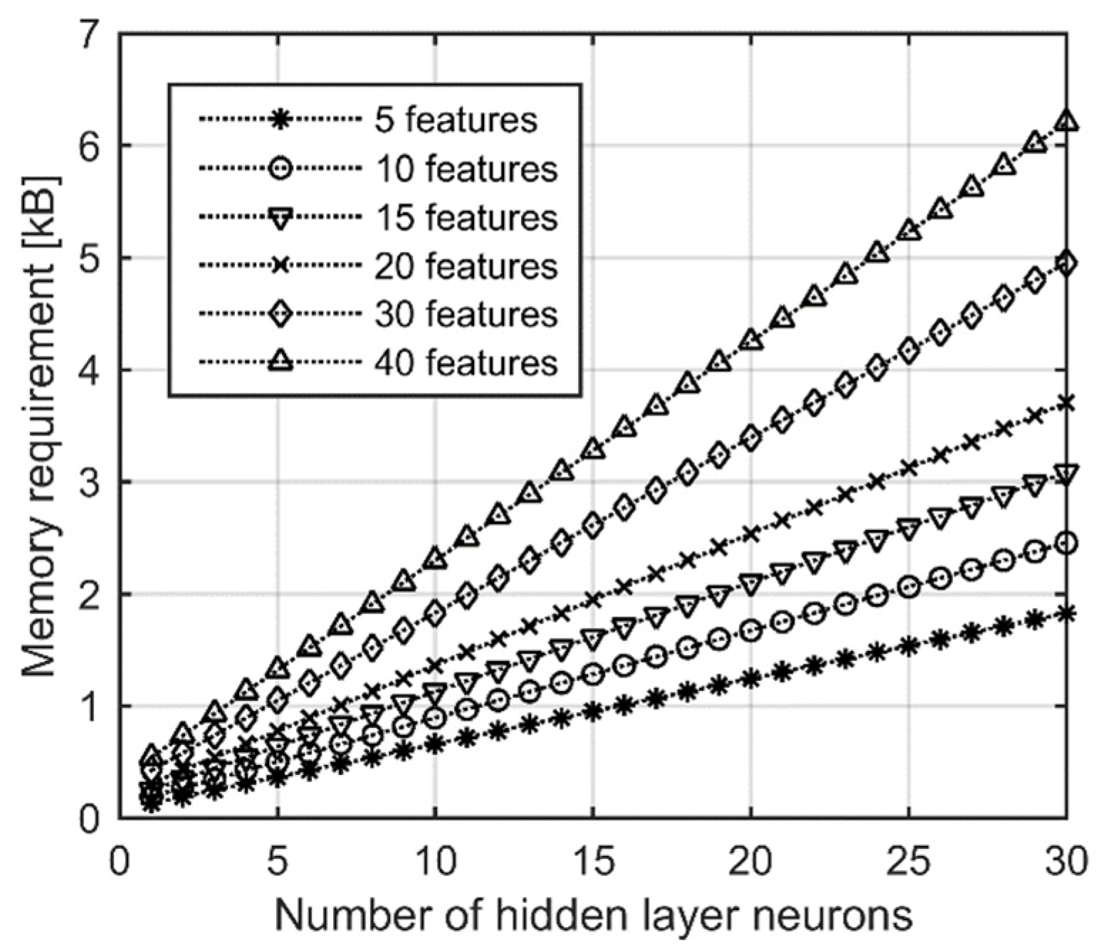
5.4. Implementation
6. Conclusions
Author Contributions
Funding
Institutional Review Board Statement
Informed Consent Statement
Data Availability Statement
Acknowledgments
Conflicts of Interest
References
- Cheung, S.; Varaiya, P. Traffic Surveillance by Wireless Sensor Networks: Final Report; University of California: Berkeley, CA, USA, 2007. [Google Scholar]
- Gheorghiu, R.A.; Iordache, V.; Stan, V.A. Urban traffic detectors—Comparison between inductive loop and magnetic sensors. In Proceedings of the International Conference on Electronics, Computers and Artificial Intelligence (ECAI), Pitesti, Romania, 29–30 June 2021. [Google Scholar] [CrossRef]
- Gajda, J.; Stencel, M. A highly selective vehicle classification utilizing dual-loop inductive detector. Metrol. Meas. Syst. 2014, 21, 473–484. [Google Scholar] [CrossRef]
- Meta, S.; Cinsdikici, M. Vehicle-classification algorithm based on component analysis for single-loop inductive detector. IEEE Trans. Veh. Technol. 2010, 59, 2795–2805. [Google Scholar] [CrossRef]
- Gajda, J.; Mielczarek, M. Automatic vehicle classification in systems with single inductive loop detector. Metrol. Meas. Syst. 2014, 21, 619–630. [Google Scholar] [CrossRef]
- Balid, W.; Tafish, H.; Refai, H. Intelligent vehicle counting and classification sensor for real-time traffic surveillance. IEEE Trans. Intell. Transp. Syst. 2018, 19, 1784–1794. [Google Scholar] [CrossRef]
- Fimbombaya, H.S.; Mvungi, N.H.; Hamisi, N.Y.; Iddi, H.U. Enhanced magnetic wireless sensor network algorithm for traffic flow monitoring in low-speed congested traffic. J. Electr. Comput. Eng. 2020, 2020, 5875398. [Google Scholar] [CrossRef]
- Feng, Y.; Zhang, J.A.; Cheng, B.; He, X.; Chen, J. Magnetic sensor-based multi-vehicle data association. IEEE Sens. J. 2021, 21, 24709–24719. [Google Scholar] [CrossRef]
- Valenti, G.; Biral, F.; Fontanelli, D. Vehicle Localisation using asphalt embedded magnetometer sensors. In Proceedings of the IEEE International Workshop on Metrology for Automotive (MetroAutomotive), Bologna, Italy, 2–3 July 2021. [Google Scholar] [CrossRef]
- Lan, J.; Xiang, Y.; Wang, L.; Shi, Y. Vehicle detection and classification by measuring and processing magnetic signal. Measurement 2011, 44, 174–180. [Google Scholar] [CrossRef]
- Wahlström, N.; Hostettler, R.; Gustafsson, F.; Birk, W. Classification of driving direction in traffic surveillance using magnetometers. IEEE Trans. Intell. Transp. Syst. 2014, 15, 1405–1418. [Google Scholar] [CrossRef]
- Zhu, Q.; Tong, G.; Li, B.; Yuan, X. A practicable method for ferromagnetic object moving direction identification. IEEE Trans. Magn. 2012, 48, 2340–2345. [Google Scholar] [CrossRef]
- Smidla, J.; Simon, G. Accelerometer-based event detector for low-power applications. Sensors 2013, 13, 13978–13997. [Google Scholar] [CrossRef] [PubMed]
- Hostettler, R.; Djurić, P. Vehicle tracking based on fusion of magnetometer and accelerometer sensor measurements with particle filtering. IEEE Trans. Veh. Technol. 2015, 64, 4917–4928. [Google Scholar] [CrossRef]
- Ma, W.; Xing, D.; McKee, A.; Bajwa, R.; Flores, C.; Fuller, B.; Varaiya, P. A wireless accelerometer-based automatic vehicle classification prototype system. IEEE Trans. Intell. Transp. Syst. 2014, 15, 104–111. [Google Scholar] [CrossRef]
- Kleyko, D.; Hostettler, R.; Birk, W.; Osipov, E. Comparison of machine learning techniques for vehicle classification using road side sensors. In Proceedings of the IEEE International Conference on Intelligent Transportation Systems (ITSC), Gran Canaria, Spain, 15–18 September 2015. [Google Scholar] [CrossRef]
- Miklusis, D.; Markevicius, V.; Navikas, D.; Cepenas, M.; Balamutas, J.; Valinevicius, A.; Zilys, M.; Cuinas, I.; Klimenta, D.; Andriukaitis, D. Research of distorted vehicle magnetic signatures recognitions, for length estimation in real traffic conditions. Sensors 2021, 21, 7872. [Google Scholar] [CrossRef]
- Zhang, Z.; Tao, M.; Yuan, H. A parking occupancy detection algorithm based on AMR sensor. IEEE Sens. J. 2015, 15, 1261–1269. [Google Scholar] [CrossRef]
- Zhu, H.; Yu, F. A vehicle parking detection method based on correlation of magnetic signals. Int. J. Distrib. Sens. Netw. 2015, 2015, 361242. [Google Scholar] [CrossRef]
- Zhu, H.; Yu, F. A cross-correlation technique for vehicle detections in wireless magnetic sensor network. IEEE Sens. J. 2016, 16, 4484–4494. [Google Scholar] [CrossRef]
- Taghvaeeyan, S.; Rajamani, R. Portable roadside sensors for vehicle counting, classification, and speed measurement. IEEE Trans. Intell. Transp. Syst. 2014, 15, 73–83. [Google Scholar] [CrossRef]
- Sifuentes, E.; Casas, O.; Pallas-Areny, R. Wireless magnetic sensor node for vehicle detection with optical wake-up. IEEE Sens. J. 2011, 11, 1669–1676. [Google Scholar] [CrossRef]
- Markevicius, V.; Navikas, D.; Zilys, M.; Andriukaitis, D.; Valinevicius, A.; Cepenas, M. Dynamic vehicle detection via the use of magnetic field sensors. Sensors 2016, 16, 78. [Google Scholar] [CrossRef]
- Burresi, G.; Giorgi, R. A field experience for a vehicle recognition system using magnetic sensors. In Proceedings of the Mediterranean Conference on Embedded Computing (MECO), Budva, Montenegro, 14–18 June 2015. [Google Scholar] [CrossRef]
- Vancin, S.; Erdem, E. Implementation of the vehicle recognition systems using wireless magnetic sensors. Sadhana 2017, 42, 841–854. [Google Scholar] [CrossRef]
- Yang, B.; Lei, Y. Vehicle detection and classification for low-speed congested traffic with anisotropic magnetoresistive sensor. IEEE Sens. J. 2015, 15, 1132–1138. [Google Scholar] [CrossRef]
- Dong, H.; Wang, X.; Zhang, C.; He, R.; Jia, L.; Qin, Y. Improved robust vehicle detection and identification based on single magnetic sensor. IEEE Access 2018, 6, 5247–5255. [Google Scholar] [CrossRef]
- Markevicius, V.; Navikas, D.; Idzkowski, A.; Andriukaitis, D.; Valinevicius, A.; Zilys, M. Practical methods for vehicle speed estimation using a microprocessor-embedded system with AMR sensors. Sensors 2018, 18, 2225. [Google Scholar] [CrossRef]
- Wang, Q.; Zheng, J.; Xu, H.; Xu, B.; Chen, R. Roadside magnetic sensor system for vehicle detection in urban environments. IEEE Trans. Intell. Transp. Syst. 2018, 19, 1365–1374. [Google Scholar] [CrossRef]
- Hodon, M.; Karpis, O.; Sevcik, P.; Kocianova, A. Which digital-output MEMS magnetometer meets the requirements of modern road traffic survey? Sensors 2021, 21, 266. [Google Scholar] [CrossRef] [PubMed]
- Spandonidis, C.; Giannopoulos, F.; Sedikos, E.; Reppas, D.; Theodoropoulos, P. Development of a MEMS-based IoV system for augmenting road traffic survey. IEEE Trans. Instrum. Meas. 2022, 71, 9510908. [Google Scholar] [CrossRef]
- Tafish, H.; Balid, W.; Refai, H. Cost effective vehicle classification using a single wireless magnetometer. In Proceedings of the International Wireless Communications and Mobile Computing Conference (IWCMC), Paphos, Cyprus, 5–9 September 2016. [Google Scholar] [CrossRef]
- Zhang, W.; Tan, G.; Ding, N.; Shang, Y.; Lin, M. Vehicle classification algorithm based on binary proximity magnetic sensors and neural network. In Proceedings of the IEEE International Conference on Intelligent Transportation Systems (ITSC), Beijing, China, 12–15 October 2008. [Google Scholar] [CrossRef]
- Velisavljevic, V.; Cano, E.; Dyo, V.; Allen, B. Wireless magnetic sensor network for road traffic monitoring and vehicle classification. Transp. Telecommun. 2016, 17, 274–288. [Google Scholar] [CrossRef]
- Wang, K.; Xiong, H.; Zhang, J.; Chen, H.; Dou, D.; Xu, C.-Z. SenseMag: Enabling low-cost traffic monitoring using non-invasive magnetic sensing. IEEE Internet Things J. 2021, 8, 16666–16679. [Google Scholar] [CrossRef]
- Xu, C.; Wang, Y.; Bao, X.; Li, F. Vehicle classification using an imbalanced dataset based on a single magnetic sensor. Sensors 2018, 18, 1690. [Google Scholar] [CrossRef]
- Zhang, X.; Huang, H. Vehicle classification based on feature selection with anisotropic magnetoresistive sensor. IEEE Sens. J. 2019, 19, 9976–9982. [Google Scholar] [CrossRef]
- Chen, X.; Kong, X.; Xu, M.; Sandrasegaran, K.; Zheng, J. Road vehicle detection and classification using magnetic field measurement. IEEE Access 2019, 7, 52622–52633. [Google Scholar] [CrossRef]
- Li, W.; Liu, Z.; Hui, Y.; Yang, L.; Chen, R.; Xiao, X. Vehicle classification and speed estimation based on a single magnetic sensor. IEEE Access 2020, 8, 126814–126824. [Google Scholar] [CrossRef]
- Li, H.; Dong, H.; Jia, L.; Ren, M. Vehicle classification with single multi-functional magnetic sensor and optimal MNS-based CART. Measurement 2014, 55, 142–152. [Google Scholar] [CrossRef]
- Feng, Y.; Mao, G.; Cheng, B.; Li, C.; Hui, Y.; Xu, Z.; Chen, J. MagMonitor: Vehicle speed estimation and vehicle classification through a magnetic sensor. IEEE Trans. Intell. Transp. Syst. 2022, 23, 1311–1322. [Google Scholar] [CrossRef]
- Kaewkamnerd, S.; Chinrungrueng, J.; Pongthornseri, R.; Dumnin, S. Vehicle classification based on magnetic sensor signal. In Proceedings of the International Conference on Information and Automation (ICIA), Harbin, China, 20–23 June 2010. [Google Scholar] [CrossRef]
- He, Y.; Du, Y.; Sun, L.; Wang, Y. Improved waveform-feature-based vehicle classification using a single-point magnetic sensor. J. Adv. Transp. 2015, 49, 663–682. [Google Scholar] [CrossRef]
- Sarcevic, P.; Pletl, S. Vehicle classification and false detection filtering using a single magnetic detector based intelligent sensor. In Proceedings of the International Conference on Information Society and Technology (ICIST), Kopaonik, Serbia, 9–13 March 2014. [Google Scholar]
- Sarcevic, P. New Methods in the Application of Inertial and Magnetic Sensors in Online Pattern Recognition Problems. Ph.D. Thesis, University of Szeged, Szeged, Hungary, 2019. [Google Scholar]
- Sarcevic, P.; Pletl, S. False detection filtering method for magnetic sensor-based vehicle detection systems. In Proceedings of the IEEE International Symposium on Intelligent Systems and Informatics (SISY), Subotica, Serbia, 13–15 September 2018. [Google Scholar] [CrossRef]
- Sarcevic, P.; Kincses, Z.; Pletl, S. Online human movement classification using wrist-worn wireless sensors. J. Ambient Intell. Humaniz. Comput. 2019, 10, 89–106. [Google Scholar] [CrossRef]


| Related Work | Sensor Placement | Vehicle Classes | Sample Number | Classifier | Efficiency |
|---|---|---|---|---|---|
| [10] | side of the road | 3 (heavy tracked vehicle; light tracked vehicle; light wheeled vehicle) | 93 | SVM | 86.27% |
| [26] | side of the road | 5 (motorcycle; hatchback; sedan; SUV; bus) | 100 | CT | 97% |
| [36] | side of the road | 4 (hatchback; sedan; bus; multi-purpose vehicle) | 300 | k-NN | 95.46% |
| [37] | side of the road | 3 (truck; saloon and SUV; bus) | 2346 | SVM | 95.36% |
| [38] | side of the road | 5 (sedan; van; truck; bus; non-vehicle) | 412 | DTW + VQ | 94.6% |
| [39] | side of the road | 7 (motorcycle; car; SUV; truck; crane; medium truck; bus) | 6042 | CNN | 97.09% |
| [1] | middle of the lane | 5 (passenger vehicle; SUV; van; pickup; bus) | 37 | Direct Hill-Pattern Matching | 63% |
| [40] | middle of the lane | 2 (car; bus) | 542 | CT | 97.0% on training data, 88.9% on validation data |
| [25] | middle of the lane | 4 (car; minibus; bus; truck) | 100 | CT | 95% |
| [27] | middle of the lane | 4 (sedan and SUV; van and seven-seat; light and medium truck; heavy truck and semi-trailer) | 4507 | CT | 80.55% on validation data |
| [41] | middle of the lane | 4 (sedan; SUV and van; bus; truck) | 115 | SVM | 87% |
| [42] | middle of the lane (1 board with 2 sensors) | 4 (motorcycle; car; van; pickup) | 130 | CT | 81.69% |
| [43] | middle of the lane (1 board with 2 sensors) | 3 (bus; small and medium truck; large truck) | 460 | SVM | 92.8% |
| [32] | atop of the roadway | 3 (passenger car, 2-axle single-unit vehicles; 2-axle and 3-axle single-unit trucks; 5-axle single-trailer trucks) | 1985 | SVM | 86.85% |
| Related Work | Data Type | Features |
|---|---|---|
| [10] | X | concavity area, convexity area, the angle of concave part, the angle of convex part of the waveform |
| [26] | X, Y | vehicle signal duration, signal energy, average energy, ratio of positive and negative energy |
| [36] | X, Y, Z, F | position of the maximum, position of the minimum, detection length, peak-to-peak value, mean value, standard deviation, number of extremes, the sign of the first extreme, the number of zero-crossings, energy of the detected signal, average energy, ratio of the energy of the signals on the sensor’s axis to the energy of the F signal, first non-zero samples of the frequency spectrum |
| [1] | X, Z | Hill-patterns |
| [40] | F | number of peaks, maximum peak time ratio, minimum trough time ratio, mean value, the standard deviation, the maximum peak amplitude, the minimum trough amplitude, maximum peak/trough amplitude ratio |
| [25] | F | magnetic signature length |
| [27] | Z | statistical features: magnetic length, mean, variance, maximum and minimum, position of the maximum and minimum, number of local maxima and minima, crossing mean counts; energy features: energy, mean energy; short-term features: mean, variance and energy computed in intra-frames of the detection window |
| [42] | Z | signal length, relative vehicle length, Hill-pattern peaks, three differential energy parameters |
| [43] | F | structural features: number of local maxima, local minima, extreme points, and negative local minima, relative time of minimum and maximum, penultimate minimum/minimum; spectrum features: highest spectrum power and the corresponding frequency; numerical features: maximum value, minimum value, sum of value, average value, max value/min value, max average value/average value, standard deviation, on-time speed |
| [37] | X, Y, Z | maximum, range, relative position of maximum, relative position of minimum, mean, ratio of positive and negative energy, number of local maxima, number of local minima, variance, approximate entropy, crossing mean counts, average energy |
| [38] | F | MFCC, energy |
| [41] | X, Y, Z | HOG features using image processing |
| [39] | X, Y, Z | 224 × 244 grayscale images containing the waveforms |
| [32] | F | FFT + PCA |
| Hyperparameter | Value |
|---|---|
| number of layers | 3 (1 input, 1 hidden, 1 output) |
| number of neurons in the input layer | the size of the feature vector |
| number of hidden layer neurons | optimal number given by the best results |
| transfer function in the hidden layer | tangent sigmoid |
| number of neurons in the output layer | the number of defined classes |
| transfer function in the output layer | linear |
| Class Number | Vehicle Types | Number of Axles |
|---|---|---|
| 1 | motorcycle | 2 |
| 2 | car | 2 |
| 3 | car with trailer | 2 + 1 |
| 4 | van, mini bus | 2 |
| 5 | truck | 2–3 |
| 6 | truck with trailer | 2–3 + 2–3 |
| 7 | tractor trailer | 2 + 3 |
| 8 | bus | 2 |
| 9 | articulated bus | 3 |
| Hyperparameter | Value |
|---|---|
| training function | Levenberg-Marquardt backpropagation |
| performance function | mean squared error (MSE) |
| maximum number of epochs to train | 5000 |
| performance goal | 0 |
| maximum validation failures | 15 |
| minimum performance gradient | 10−7 |
| maximum time to train in seconds | inf |
| Used Axes | |||||||||||
|---|---|---|---|---|---|---|---|---|---|---|---|
| Feature Number | |||||||||||
| Efficiency on Training Data | Efficiency on Validation Data | ||||||||||
| X, Y, Z | X, Y, Z, DL | X | X, DL | Z | Z, DL | ||||||
| 42 | 43 | 14 | 15 | 14 | 15 | ||||||
| 82.11 | 67.69 | 81.50 | 66.58 | 78.83 | 71.33 | 80.11 | 72.22 | 77.92 | 71.24 | 81.36 | 72.36 |
| X, Z | X, Z, DL | Xabs, Yabs, Zabs | Xabs, Yabs, Zabs, DL | Xabs | Xabs, DL | ||||||
| 28 | 29 | 27 | 28 | 9 | 10 | ||||||
| 81.61 | 70.13 | 81.97 | 71.64 | 81.00 | 71.20 | 81.81 | 69.73 | 73.86 | 68.18 | 76.14 | 70.04 |
| Zabs | Zabs, DL | Xabs, Zabs | Xabs, Zabs, DL | XYO, XZO, YZO, XYZO | XYO, XZO, YZO, XYZO, DL | ||||||
| 9 | 10 | 18 | 19 | 56 | 57 | ||||||
| 74.31 | 69.07 | 75.56 | 69.82 | 78.97 | 69.96 | 80.08 | 71.38 | 82.20 | 70.18 | 82.81 | 68.18 |
| XZO | XZO, DL | XYO, XZO, YZO | XYO, XZO, YZO, DL | XYZO | XYZO, DL | ||||||
| 14 | 15 | 42 | 43 | 14 | 15 | ||||||
| 80.75 | 73.73 | 80.14 | 74.44 | 81.03 | 69.82 | 84.06 | 71.51 | 77.97 | 72.76 | 81.39 | 74.67 |
| XYA, XZA, YZA | XYA, XZA, YZA, DL | XZA | XZA, DL | XYC, XZC, YZC, XYZC | XYC, XZC, YZC, XYZC, DL | ||||||
| 42 | 43 | 14 | 15 | 36 | 37 | ||||||
| 79.00 | 66.53 | 79.97 | 65.78 | 80.92 | 71.20 | 79.69 | 71.87 | 79.08 | 66.36 | 81.75 | 69.11 |
| XZC | XZC, DL | XYC, XZC, YZC | XYC, XZC, YZC, DL | XYZC | XYZC, DL | ||||||
| 9 | 10 | 27 | 28 | 9 | 10 | ||||||
| 72.78 | 68.49 | 76.53 | 70.53 | 80.83 | 68.36 | 79.28 | 68.27 | 73.61 | 68.93 | 75.69 | 71.38 |
| Output Class | Sum | ||||||||||
|---|---|---|---|---|---|---|---|---|---|---|---|
| 1 | 2 | 3 | 4 | 5 | 6 | 7 | 8 | 9 | |||
| Target class | 1 | 1.6 | 0.4 | 1.2 | 3.2 | ||||||
| 2.8 | 0.4 | 3.2 | |||||||||
| 2 | 2.0 | 2.8 | 4.8 | 0.4 | 10.0 | ||||||
| 2.0 | 2.4 | 6.8 | 1.2 | 12.4 | |||||||
| 3 | 4.8 | 7.2 | 10.8 | 1.2 | 1.2 | 25.2 | |||||
| 7.2 | 10.0 | 10.8 | 0.4 | 0.4 | 1.2 | 30.0 | |||||
| 4 | 0.8 | 10.4 | 7.6 | 24.0 | 0.4 | 1.6 | 44.8 | ||||
| 0.8 | 17.6 | 8.0 | 24.0 | 1.6 | 52.0 | ||||||
| 5 | 0.8 | 6.0 | 10.8 | 0.8 | 2.8 | 12.4 | 1.2 | 34.8 | |||
| 1.2 | 4.8 | 8.4 | 0.8 | 2.8 | 18.0 | 0.4 | 36.4 | ||||
| 6 | 0.8 | 0.4 | 2.4 | 16.8 | 4.4 | 13.2 | 38.0 | ||||
| 2.0 | 1.6 | 21.6 | 4.0 | 11.6 | 40.8 | ||||||
| 7 | 1.6 | 0.4 | 2.4 | 13.6 | 12.8 | 8.4 | 39.2 | ||||
| 0.4 | 2.0 | 16.4 | 10.8 | 9.6 | 39.2 | ||||||
| 8 | 0.8 | 3.2 | 1.2 | 3.6 | 2.4 | 11.2 | |||||
| 0.4 | 4.0 | 0.8 | 4.0 | 4.4 | 13.6 | ||||||
| 9 | 0.4 | 8.8 | 2.8 | 11.6 | 23.6 | ||||||
| 0.4 | 6.8 | 4.0 | 5.6 | 16.8 | |||||||
| Hidden Layer Neuron Number | 5 | 10 | 15 | 20 | 25 | 30 |
| Percentage of Convergence For Training Data | 0.00% | 2.78% | 19.44% | 30.56% | 38.89% | 8.33% |
| Percentage of Convergence For Validation Data | 0.00% | 58.33% | 30.56% | 8.33% | 2.78% | 0.00% |
Publisher’s Note: MDPI stays neutral with regard to jurisdictional claims in published maps and institutional affiliations. |
© 2022 by the authors. Licensee MDPI, Basel, Switzerland. This article is an open access article distributed under the terms and conditions of the Creative Commons Attribution (CC BY) license (https://creativecommons.org/licenses/by/4.0/).
Share and Cite
Sarcevic, P.; Pletl, S.; Odry, A. Real-Time Vehicle Classification System Using a Single Magnetometer. Sensors 2022, 22, 9299. https://doi.org/10.3390/s22239299
Sarcevic P, Pletl S, Odry A. Real-Time Vehicle Classification System Using a Single Magnetometer. Sensors. 2022; 22(23):9299. https://doi.org/10.3390/s22239299
Chicago/Turabian StyleSarcevic, Peter, Szilveszter Pletl, and Akos Odry. 2022. "Real-Time Vehicle Classification System Using a Single Magnetometer" Sensors 22, no. 23: 9299. https://doi.org/10.3390/s22239299
APA StyleSarcevic, P., Pletl, S., & Odry, A. (2022). Real-Time Vehicle Classification System Using a Single Magnetometer. Sensors, 22(23), 9299. https://doi.org/10.3390/s22239299