

EEG-Based Emotion Classification Using Stacking Ensemble Approach


Abstract
1. Introduction
- An advance ensemble model developed with random forest, light gradient boosting machine, and gradient-boosting-based stacking ensemble (RLGB-SE) classifier models is proposed to classify various emotional states.
- A new method of categorizing emotions into three categories (positive, neutral, and negative) allows for real-world mental states that are not primarily characterized by emotions.
- We conduct a comparison to validate the performance of the proposed ensemble model with advanced ML models and various ensemble model combinations.
2. Related Works
3. Methodology
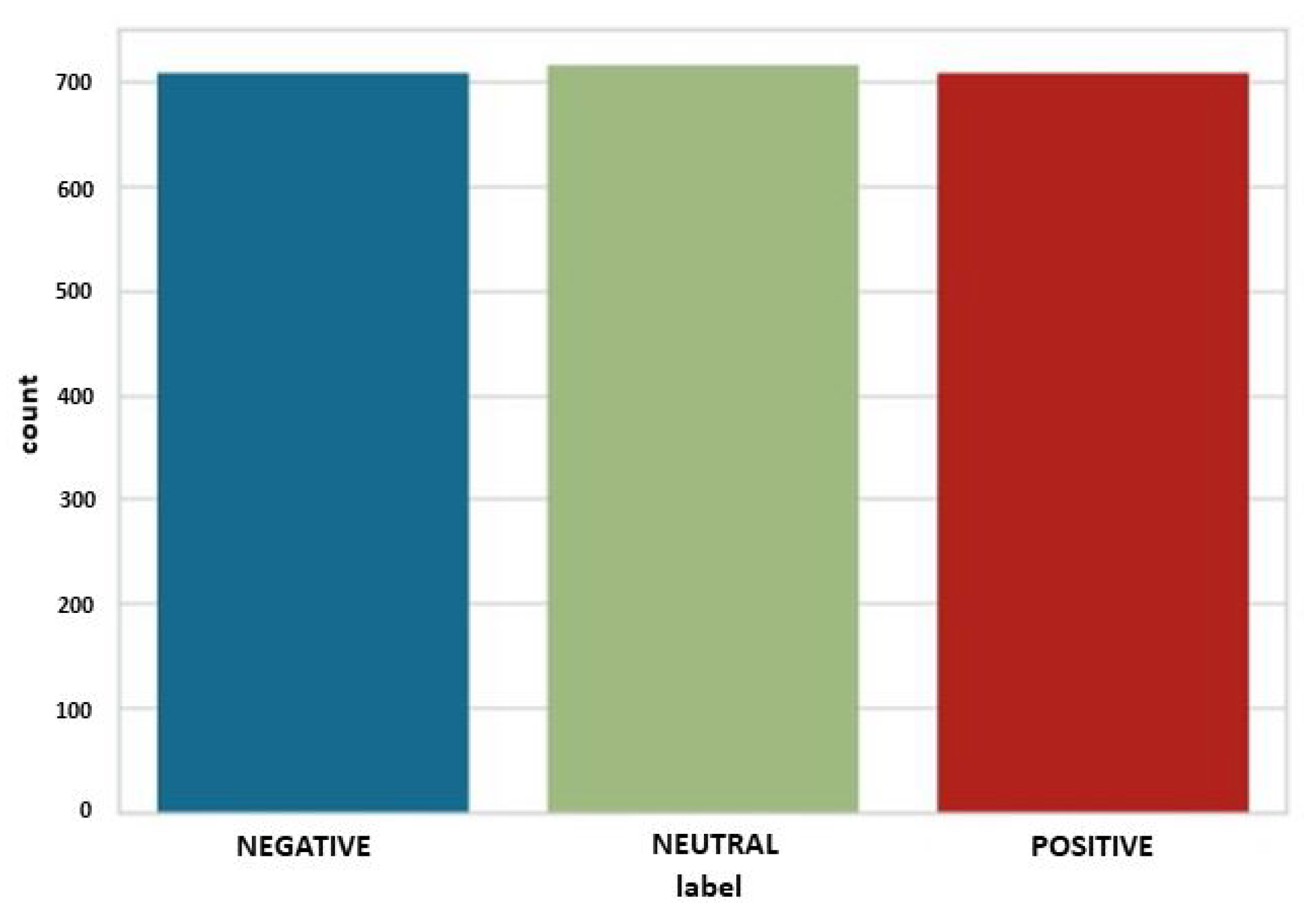
3.1. Data Analysis
3.2. Design of Stacking Ensemble Model
| Algorithm 1 Pseudocode of the proposed stacking ensemble strategy. |
|
3.2.1. Random Forest
3.2.2. Light Gradient Boosting Machine
3.2.3. Gradient Boosting Classifier
4. Results
4.1. Comparison with Confusion Matrix
4.2. Classification Result Compared with Different Models
5. Conclusions
Author Contributions
Funding
Institutional Review Board Statement
Informed Consent Statement
Data Availability Statement
Conflicts of Interest
Abbreviations
| EEG | Electroencephalography |
| ECoG | Electrocorticography |
| BCI | Brain–Computer Interface |
| RF | Random Forest |
| LightGBM | Light Gradient Boosting Machine |
| GBC | Gradient Boosting Classifier |
| ROC | Receiver Operation Characteristics |
| LSTM | Long Short-Term Memory |
| LDS | Linear Dynamical System |
| MRMR | Minimal-Redundancy-Maximal-Relevance |
| SVM | Support Vector Machine |
| KNN | K-nearest neighbors |
| CSP | Common Spatial Patterns |
| fMRI | Functional Magnetic Resonance Imaging |
| DWT | Discrete Wavelet Transform |
| LDA | Linear Discriminant Analysis |
References
- Mauss, I.B.; Robinson, M.D. Measures of emotion: A review. Cogn. Emot. 2009, 23, 209–237. [Google Scholar] [CrossRef]
- Zhong, P.; Wang, D.; Miao, C. EEG-based emotion recognition using regularized graph neural networks. IEEE Trans. Affect. Comput. 2020, 13, 1290–1301. [Google Scholar] [CrossRef]
- Ranganathan, H.; Chakraborty, S.; Panchanathan, S. Multimodal emotion recognition using deep learning architectures. In Proceedings of the 2016 IEEE Winter Conference on Applications of Computer Vision (WACV), Lake Placid, NY, USA, 7–10 March 2016; IEEE: Piscataway, NJ, USA, 2016; pp. 1–9. [Google Scholar]
- Petrushin, V. Emotion in speech: Recognition and application to call centers. In Proceedings of the Artificial Neural Networks in Engineering; Springer: Berlin/Heidelberg, Germany, 1999; Volume 710, p. 22. [Google Scholar]
- Black, M.J.; Yacoob, Y. Recognizing facial expressions in image sequences using local parameterized models of image motion. Int. J. Comput. Vis. 1997, 25, 23–48. [Google Scholar] [CrossRef]
- Anderson, K.; McOwan, P.W. A real-time automated system for the recognition of human facial expressions. IEEE Trans. Syst. Man Cybern. Part Cybern. 2006, 36, 96–105. [Google Scholar] [CrossRef]
- Coan, J.A.; Allen, J.J. Frontal EEG asymmetry as a moderator and mediator of emotion. Biol. Psychol. 2004, 67, 7–50. [Google Scholar] [CrossRef]
- Li, X.; Hu, B.; Zhu, T.; Yan, J.; Zheng, F. Towards affective learning with an EEG feedback approach. In Proceedings of the First ACM International Workshop on Multimedia Technologies for Distance Learning, Beijing, China, 23 October 2009; pp. 33–38. [Google Scholar]
- Davidson, R.J.; Fox, N.A. Asymmetrical brain activity discriminates between positive and negative affective stimuli in human infants. Science 1982, 218, 1235–1237. [Google Scholar] [CrossRef]
- Yuen, C.T.; San San, W.; Seong, T.C.; Rizon, M. Classification of human emotions from EEG signals using statistical features and neural network. Int. J. Integr. Eng. 2009, 1, 3. [Google Scholar]
- Tanaka, H.; Hayashi, M.; Hori, T. Statistical features of hypnagogic EEG measured by a new scoring system. Sleep 1996, 19, 731–738. [Google Scholar] [CrossRef]
- Alhagry, S.; Fahmy, A.A.; El-Khoribi, R.A. Emotion recognition based on EEG using LSTM recurrent neural network. Int. J. Adv. Comput. Sci. Appl. 2017, 8, 10. [Google Scholar] [CrossRef]
- Cheng, J.; Chen, M.; Li, C.; Liu, Y.; Song, R.; Liu, A.; Chen, X. Emotion recognition from multi-channel eeg via deep forest. IEEE J. Biomed. Health Inform. 2020, 25, 453–464. [Google Scholar] [CrossRef]
- Lin, W.; Li, C.; Sun, S. Deep convolutional neural network for emotion recognition using EEG and peripheral physiological signal. In Proceedings of the International Conference on Image and Graphics; Springer: Berlin, Germany, 2017; pp. 385–394. [Google Scholar]
- Zheng, W.L.; Lu, B.L. Investigating critical frequency bands and channels for EEG-based emotion recognition with deep neural networks. IEEE Trans. Auton. Ment. Dev. 2015, 7, 162–175. [Google Scholar] [CrossRef]
- Duan, R.N.; Zhu, J.Y.; Lu, B.L. Differential entropy feature for EEG-based emotion classification. In Proceedings of the 2013 6th International IEEE/EMBS Conference on Neural Engineering (NER), San Diego, CA, USA, 6–8 November 2013; pp. 81–84. [Google Scholar]
- Fan, J.; Wade, J.W.; Bian, D.; Key, A.P.; Warren, Z.E.; Mion, L.C.; Sarkar, N. A Step towards EEG-based brain computer interface for autism intervention. In Proceedings of the 2015 37th Annual International Conference of the IEEE Engineering in Medicine and Biology Society (EMBC), Milan, Italy, 25–29 August 2015; pp. 3767–3770. [Google Scholar]
- Schupp, H.T.; Cuthbert, B.N.; Bradley, M.M.; Cacioppo, J.T.; Ito, T.; Lang, P.J. Affective picture processing: The late positive potential is modulated by motivational relevance. Psychophysiology 2000, 37, 257–261. [Google Scholar] [CrossRef]
- Pizzagalli, D.; Regard, M.; Lehmann, D. Rapid emotional face processing in the human right and left brain hemispheres: An ERP study. Neuroreport 1999, 10, 2691–2698. [Google Scholar] [CrossRef]
- Eimer, M.; Holmes, A. An ERP study on the time course of emotional face processing. Neuroreport 2002, 13, 427–431. [Google Scholar] [CrossRef]
- Chanel, G.; Kronegg, J.; Grandjean, D.; Pun, T. Emotion assessment: Arousal evaluation using EEG’s and peripheral physiological signals. In Proceedings of the International Workshop on Multimedia Content Representation, Classification and Security, Istanbul, Turkey, 11 September 2006; Springer: Berlin/Heidelberg, Germany, 2006; pp. 530–537. [Google Scholar]
- Li, M.; Lu, B.L. Emotion classification based on gamma-band EEG. In Proceedings of the 2009 Annual International Conference of the IEEE Engineering in Medicine and Biology Society, Minneapolis, MN, USA, 3–6 September 2009; IEEE: Piscataway, NJ, USA, 2009; pp. 1223–1226. [Google Scholar]
- Zhang, Q.; Lee, M. Analysis of positive and negative emotions in natural scene using brain activity and GIST. Neurocomputing 2009, 72, 1302–1306. [Google Scholar] [CrossRef]
- Murugappan, M.; Ramachandran, N.; Sazali, Y. Classification of human emotion from EEG using discrete wavelet transform. J. Biomed. Sci. Eng. 2010, 3, 390. [Google Scholar] [CrossRef]
- Petrantonakis, P.C.; Hadjileontiadis, L.J. Emotion recognition from EEG using higher order crossings. IEEE Trans. Inf. Technol. Biomed. 2009, 14, 186–197. [Google Scholar] [CrossRef]
- Bird, J.J.; Manso, L.J.; Ribeiro, E.P.; Ekárt, A.; Faria, D.R. A study on mental state classification using eeg-based brain-machine interface. In Proceedings of the 2018 International Conference on Intelligent Systems (IS), Funchal, Portugal, 25–27 September 2018; pp. 795–800. [Google Scholar]
- Bird, J.J.; Ekart, A.; Buckingham, C.D.; Faria, D.R. Mental emotional sentiment classification with an eeg-based brain-machine interface. In Proceedings of the International Conference on Digital Image and Signal Processing (DISP’19), Oxford, UK, 29–30 April 2019. [Google Scholar]
- Ali, L.; Chakraborty, C.; He, Z.; Cao, W.; Imrana, Y.; Rodrigues, J.J. A novel sample and feature dependent ensemble approach for Parkinson’s disease detection. In Neural Computing and Applications; Springer: Berlin/Heidelberg, Germany, 2022; pp. 1–14. [Google Scholar]
- Chakravarthi, B.; Ng, S.C.; Ezilarasan, M.; Leung, M.F. EEG-based Emotion Recognition Using Hybrid CNN and LSTM Classification. Front. Comput. Neurosci. 2022. epub ahead of print. [Google Scholar] [CrossRef]
- Zhong, J.; Zeng, X.; Cao, W.; Wu, S.; Liu, C.; Yu, Z.; Wong, H.S. Semisupervised Multiple Choice Learning for Ensemble Classification. IEEE Trans. Cybern. 2020, 52, 3658–3668. [Google Scholar] [CrossRef]
- Niedermeyer, E.; da Silva, F.L. Electroencephalography: Basic Principles, Clinical Applications, and Related Fields; Lippincott Williams & Wilkins: New York, NY, USA, 2005; pp. 654–660. ISBN 978-0781789424. [Google Scholar]
- Bird, J.J.; Faria, D.R.; Manso, L.J.; Ekárt, A.; Buckingham, C.D. A deep evolutionary approach to bioinspired classifier optimisation for brain-machine interaction. Complexity 2019, 2019, 1–14. [Google Scholar] [CrossRef]
- Jasper, H.H. The ten-twenty electrode system of the International Federation. Electroencephalogr. Clin. Neurophysiol. 1958, 10, 370–375. [Google Scholar]
- Witten, I.H.; Frank, E. Data mining: Practical machine learning tools and techniques with Java implementations. Acm Sigmod Rec. 2002, 31, 76–77. [Google Scholar] [CrossRef]
- Dev, V.A.; Datta, S.; Chemmangattuvalappil, N.G.; Eden, M.R. Comparison of tree based ensemble machine learning methods for prediction of rate constant of Diels-Alder reaction. In Computer Aided Chemical Engineering; Elsevier: Amsterdam, The Netherlands, 2017; Volume 40, pp. 997–1002. [Google Scholar]
- Rokach, L. Decision forest: Twenty years of research. Inf. Fusion 2016, 27, 111–125. [Google Scholar] [CrossRef]
- Sagi, O.; Rokach, L. Ensemble learning: A survey. Wiley Interdiscip. Rev. Data Min. Knowl. Discov. 2018, 8, e1249. [Google Scholar] [CrossRef]
- Kuncheva, L.I. Combining Pattern Classifiers: Methods and Algorithms; John Wiley & Sons: Hoboken, NJ, USA, 2014. [Google Scholar]
- Ensemble Methods:Bagging, Boosting and Stacking. Available online: https://towardsdatascience.com/ensemble-methods-bagging-boosting-and-stacking-c9214a10a205 (accessed on 4 September 2022).
- Acosta-Escalante, F.D.; Beltrán-Naturi, E.; Boll, M.C.; Hernández-Nolasco, J.A.; García, P.P. Meta-classifiers in Huntington’s disease patients classification, using iPhone’s movement sensors placed at the ankles. IEEE Access 2018, 6, 30942–30957. [Google Scholar] [CrossRef]
- Breiman, L. Random forests. Mach. Learn. 2001, 45, 5–32. [Google Scholar] [CrossRef]
- Biau, G.; Scornet, E. A random forest guided tour. Test 2016, 25, 197–227. [Google Scholar] [CrossRef]
- Belgiu, M.; Drăguţ, L. Random forest in remote sensing: A review of applications and future directions. ISPRS J. Photogramm. Remote Sens. 2016, 114, 24–31. [Google Scholar] [CrossRef]
- Ke, G.; Meng, Q.; Finley, T.; Wang, T.; Chen, W.; Ma, W.; Ye, Q.; Liu, T.Y. Lightgbm: A highly efficient gradient boosting decision tree. In Proceedings of the Advances in Neural Information Processing Systems, Long Beach, CA, USA, 4–9 December 2017; Volume 30, pp. 3147–3155. [Google Scholar]
- Friedman, J.H. Greedy function approximation: A gradient boosting machine. Ann. Stat. 2001, 29, 1189–1232. [Google Scholar] [CrossRef]
- Yansari, R.T.; Mirzarezaee, M.; Sadeghi, M.; Araabi, B.N. A new survival analysis model in adjuvant Tamoxifen-treated breast cancer patients using manifold-based semi-supervised learning. J. Comput. Sci. 2022, 61, 101645. [Google Scholar] [CrossRef]


| Sl No. | Film Name | Emotion Labels | Scene | Studio Name | Year |
|---|---|---|---|---|---|
| 1 | Marley and Me | Negative | Death Scene | Twentieth Century Fox | 2008 |
| 2 | Up | Negative | Opening Death Scene | Walt Disney Pictures | 2009 |
| 3 | My Girl | Negative | Funeral Scene | Imagine Entertainment | 1991 |
| 4 | La La Land | Positive | Opening musical number | Summit Entertainment | 2016 |
| 5 | Slow Life | Positive | Nature timelapse | BioQuest Studios | 2014 |
| 6 | Funny Dogs | Positive | Funny dog clips | MashupZone | 2015 |
| Sl. No. | Parameter | Random Forest | LightGBM | GBC |
|---|---|---|---|---|
| 1 | learning_rate | - | 0.2 | 0.3 |
| 2 | bagging_fraction | - | 0.6 | - |
| 3 | bagging_freq | - | 3 | - |
| 4 | n_estimators | 100 | 100 | 270 |
| 5 | feature_fraction | - | 0.9 | - |
| 6 | num_leaves | - | 90 | - |
| 7 | min_samples_leaf | 1 | - | 2 |
| 8 | min_samples_split | 2 | - | 7 |
| 9 | max_features | auto | - | sqrt |
| Sl No. | Model | Accuracy | Recall | Precision | F-Measure |
|---|---|---|---|---|---|
| 1 | Gradient Boosting Classifier | 0.9873 | 0.9870 | 0.9874 | 0.9873 |
| 2 | Light Gradient Boosting Machine | 0.9873 | 0.9870 | 0.9874 | 0.9873 |
| 3 | Random Forest Classifier | 0.9859 | 0.9857 | 0.9862 | 0.9859 |
| 4 | Extra Trees Classifier | 0.9765 | 0.9759 | 0.9773 | 0.9765 |
| 5 | Decision Tree Classifier | 0.9631 | 0.9626 | 0.9637 | 0.9631 |
| 6 | Ada Boost Classifier | 0.8297 | 0.8309 | 0.8604 | 0.8217 |
| 7 | K Neighbors Classifier | 0.7506 | 0.7447 | 0.7434 | 0.7418 |
| 8 | Voting classifier | 0.9891 | 0.9898 | 0.9893 | 0.9891 |
| 9 | Proposed Stacking model | 0.9955 | 0.9954 | 0.9953 | 0.9953 |
| Methods | Accuracy |
|---|---|
| Random Tree | 79.21 |
| Deep Belief Network | 88.66 |
| Multi-layer Perceptron classifier | 84.95 |
| Recurrent Neural Network | 87.65 |
| Proposed method | 99.55 |
Publisher’s Note: MDPI stays neutral with regard to jurisdictional claims in published maps and institutional affiliations. |
© 2022 by the authors. Licensee MDPI, Basel, Switzerland. This article is an open access article distributed under the terms and conditions of the Creative Commons Attribution (CC BY) license (https://creativecommons.org/licenses/by/4.0/).
Share and Cite
Chatterjee, S.; Byun, Y.-C. EEG-Based Emotion Classification Using Stacking Ensemble Approach. Sensors 2022, 22, 8550. https://doi.org/10.3390/s22218550
Chatterjee S, Byun Y-C. EEG-Based Emotion Classification Using Stacking Ensemble Approach. Sensors. 2022; 22(21):8550. https://doi.org/10.3390/s22218550
Chicago/Turabian StyleChatterjee, Subhajit, and Yung-Cheol Byun. 2022. "EEG-Based Emotion Classification Using Stacking Ensemble Approach" Sensors 22, no. 21: 8550. https://doi.org/10.3390/s22218550
APA StyleChatterjee, S., & Byun, Y.-C. (2022). EEG-Based Emotion Classification Using Stacking Ensemble Approach. Sensors, 22(21), 8550. https://doi.org/10.3390/s22218550