
G2O-Pose: Real-Time Monocular 3D Human Pose Estimation Based on General Graph Optimization


Abstract
1. Introduction
- Bone proportion recovery algorithm based on multiple 2D poses. No matter how the human body moves, the proportions and lengths of the human bone segments remain unchanged. Aiming at this feature, this paper studies the algorithm of recovering the proportions of the 3D bone segments from multiframe 2D poses. The average proportion error of the bones is 0.012 (calculated by the ground truth 2D keypoints, and the spine segment is used as the proportion 1).
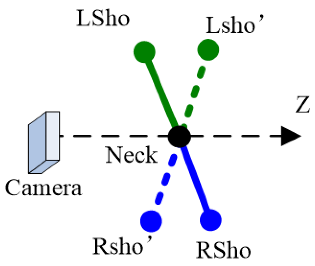
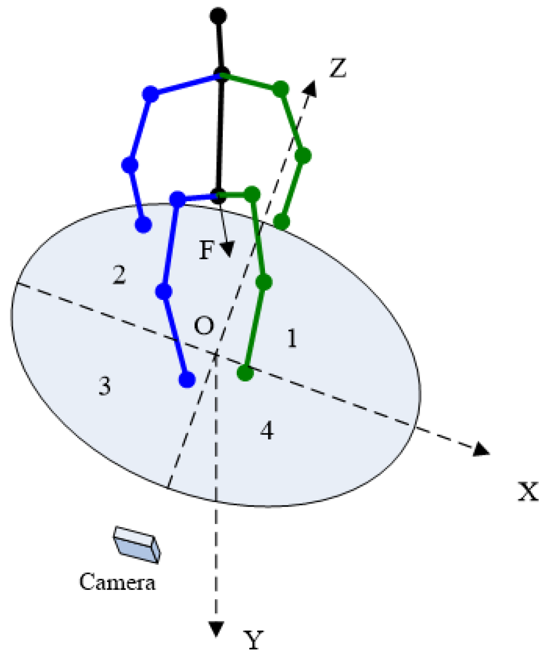
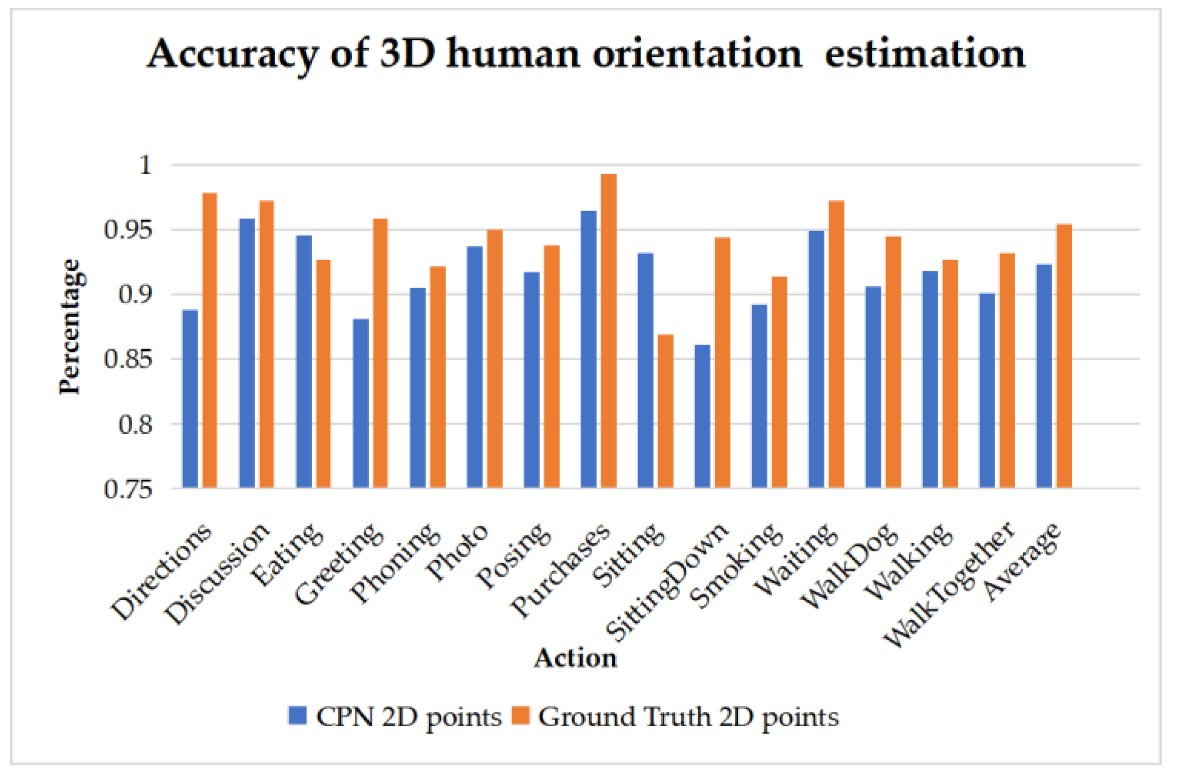
- Three-dimensional human orientation classification algorithm based on 2D joint features. Aiming at the problem of the depth ambiguity of two shoulders (or hips) keypoints, the 3D orientation of human body is estimated by 2D pose features. The accuracy of the classification reaches 95.4% (ground truth 2D key points).
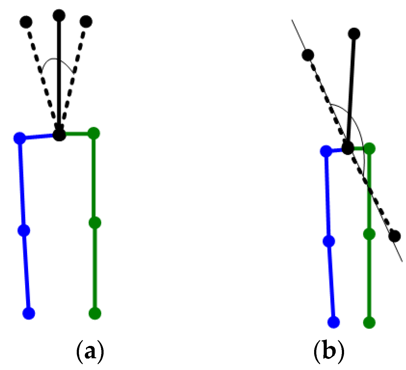
- Reverse joint correction algorithm based on heuristic search. The front and back of joint rotation are difficult to be distinguished in 2D images. Therefore, the detection, correction and suppression algorithm of the reverse joints based on rotation angles are studied, and the average accuracy of the corrections is more than 80%.
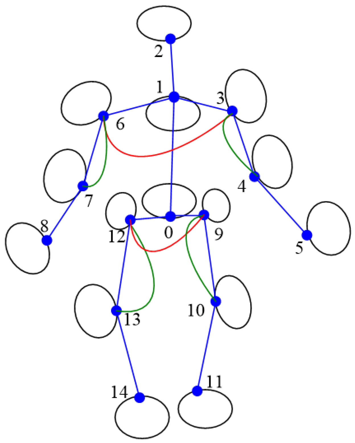
- Three-dimensional human pose estimation method based on graph optimization under multiple constraints. The 3D keypoints of human body are modeled as a graph. Under the constraints of algorithm 1–3, the 3D pose of the next frame is solved in turn with the previous pose as initial solution. The accuracy of our method is comparable to that of the previous traditional methods while the speed is greatly improved, when the depth of the human body does not change so much.
2. Related Works
2.1. Traditional Methods
2.1.1. Generative Approaches
2.1.2. Discriminative Approaches
2.1.3. Hybrid Approaches
2.2. Deep Learning-Based Methods
3. Algorithm
| Algorithm 1: Algorithm G2O-Pose |
| Input. 2D poses, camera parameters. Output. 3D poses. Step 1. Preprocess: calculate 3D bone segment proportions. Suppose the depth of the body (randomly) and calculate the lengths of bone segments. Step 2. Initialize the G2O optimizer, and the initial 3D pose. While (the depth change of the body is less than T), repeat Step 3–Step 7. Step 3. Calculate 3D body orientation. Step 4. Correct reverse joints of legs. Step 5. Solve 3D coordinates of the legs by optimization with the previous 3D pose as initial solution. Step 6. Correct reverse joints of the spine and arms. Step 7. Solve 3D coordinates of the upper part of body by optimization. |
3.1. Three-Dimensional Bone Proportion Recovery and Length Calculation Algorithm Based on Multiple 2D Poses
3.1.1. Three-Dimensional Bone Proportion Recovery
3.1.2. Recovery of 3D Bone Length with Preset Depth
- (1)
- Calculate the length of spine from a single frame
- (2)
- Calculate the average spine length by multiple frames
- (3)
- Calculate lengths of other bone segments according to the obtained bone proportions, i.e.,
3.2. Three-Dimensional Human Orientation Classification Algorithm Based on Weighted 2D Joint Features
3.3. Reverse Joint Correction Algorithm Based on Heuristic Search
3.3.1. Reverse Joint Correction Algorithm for Legs
3.3.2. Upper Body Reverse Joint Correction Algorithm
- (1)
- Correction algorithm of Neck point based on increasing confidence
- (2)
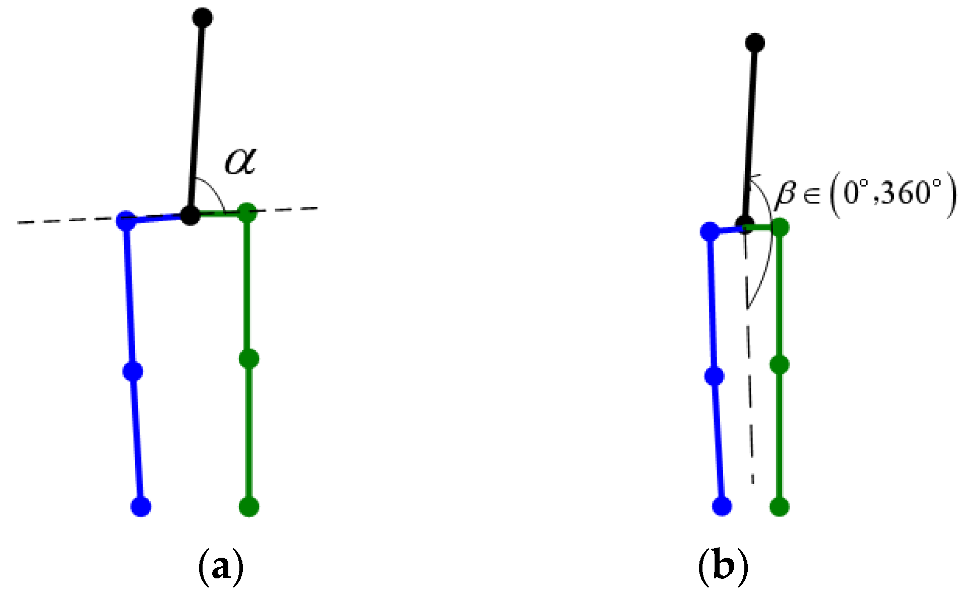
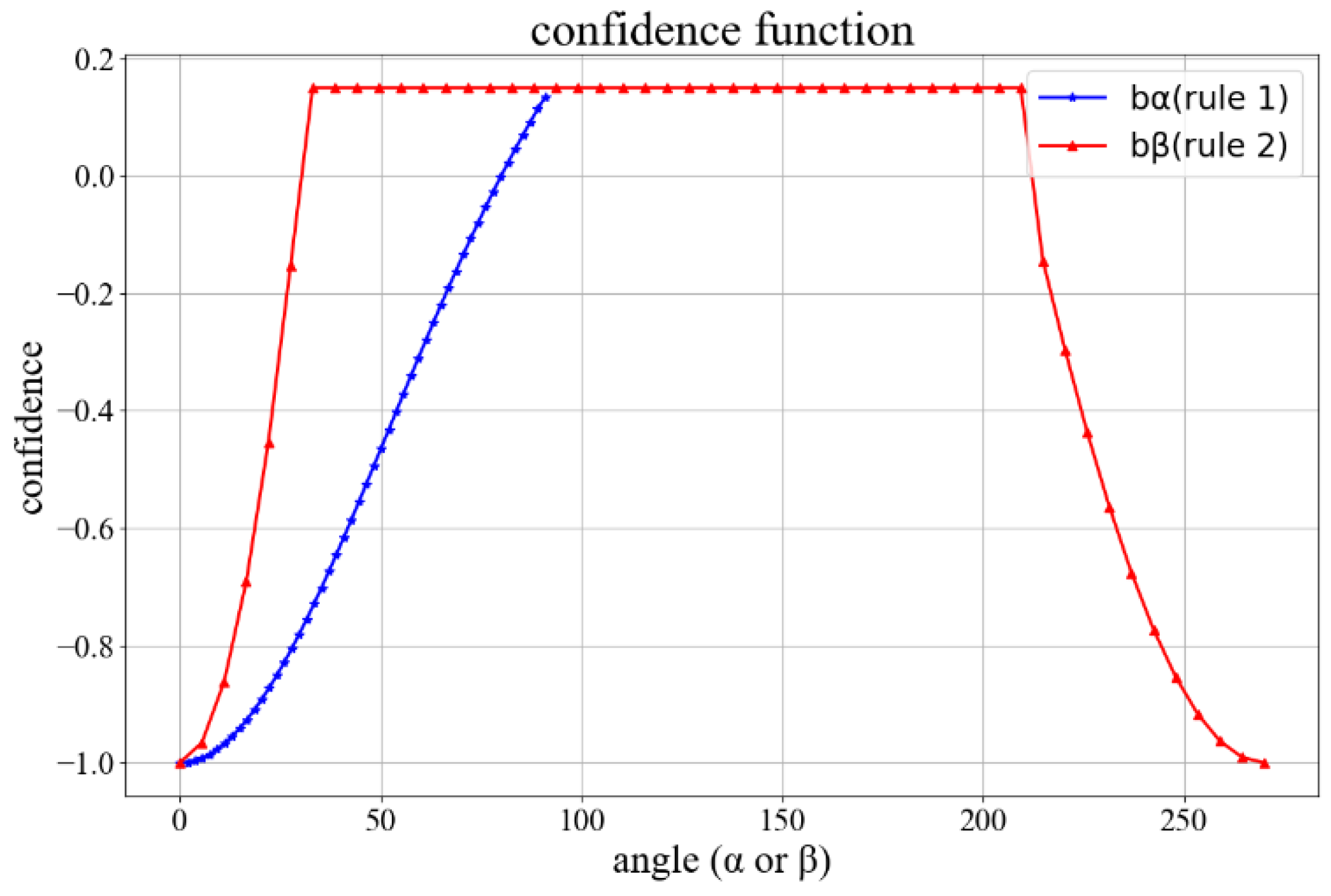
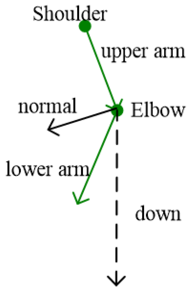
- Correction algorithm for reverse joints of arms
3.3.3. Reverse Joint Suppression Algorithm
- (1)
- For legs
- (2)
- For arms
3.4. Graph Optimization Algorithm Based on Multiple Constraints
- (1)
- Reprojection losswhere is the coordinate of the ith 3D keypoint projected onto the 2D image according to the pinhole camera model; is the 2D keypoint extracted through CPN [9] or other methods; is the coordinate of the 3D keypoint to be solved; K is the intrinsic matrix of the camera; is the projection error of the keypoint.
- (2)
- Length losswhere represents the 3D bone length solved according to Section 3.1.2, and is the current distance between keypoints the bone connected (.
- (3)
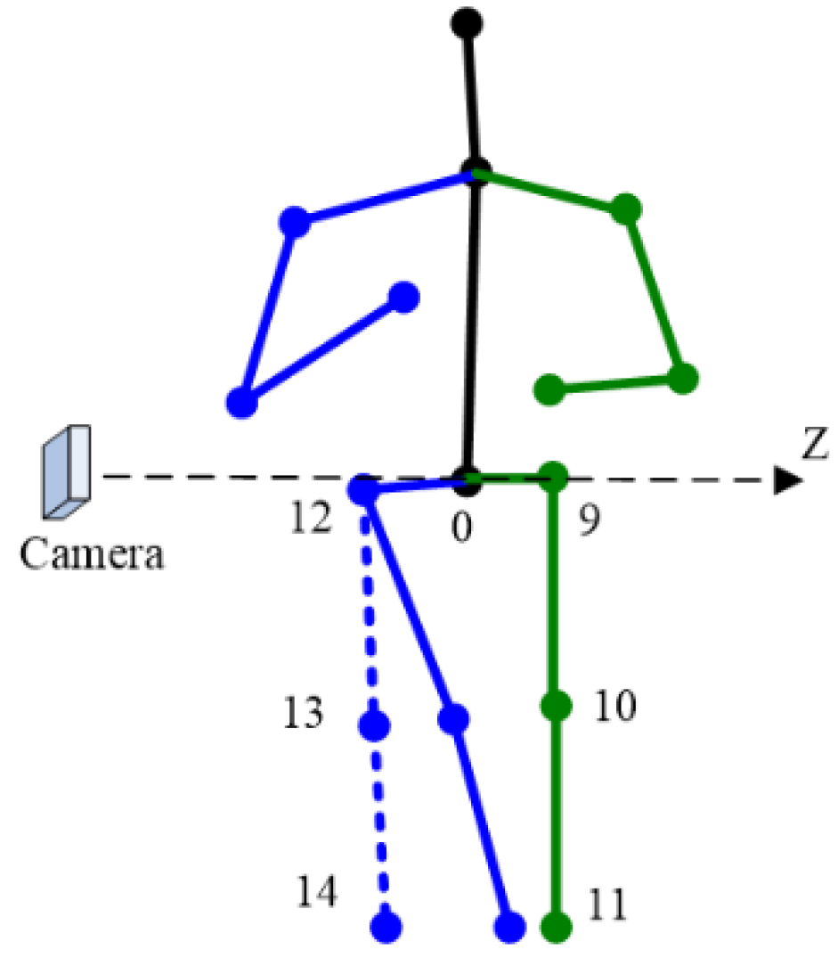
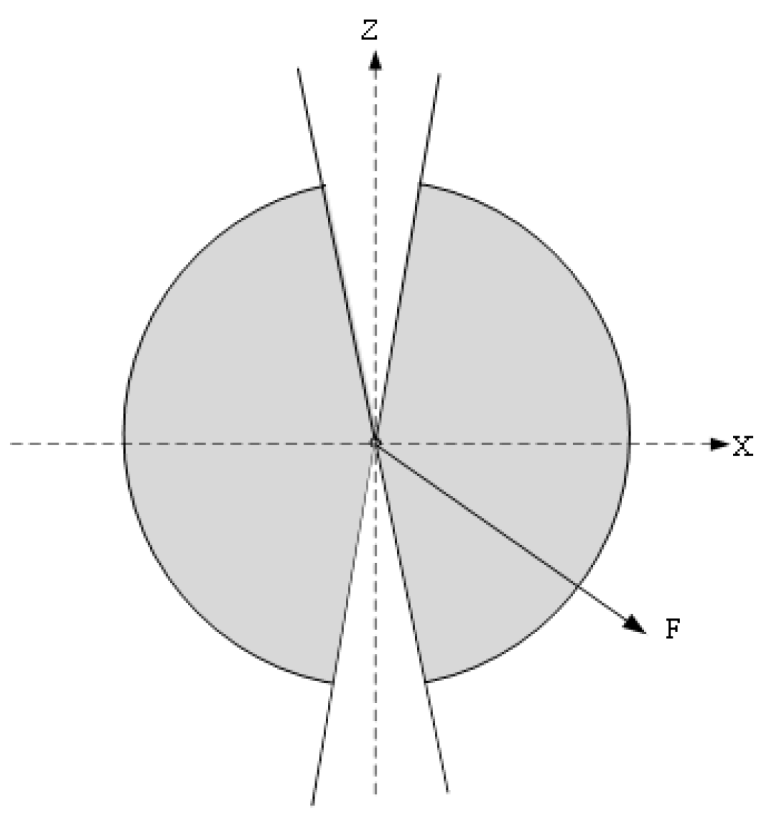
- Orientation losswhere denotes the upper body orientation constraint and denotes the lower body constraint.where is defined in Equation (20), is defined in Equation (11), , , , denotes the depth of Left Shoulder, Right Shoulder, Left Hip and Right Hip, respectively. When > 0, the depths of left limbs are expected to be larger than those of right limbs and vice versa.
- (4)
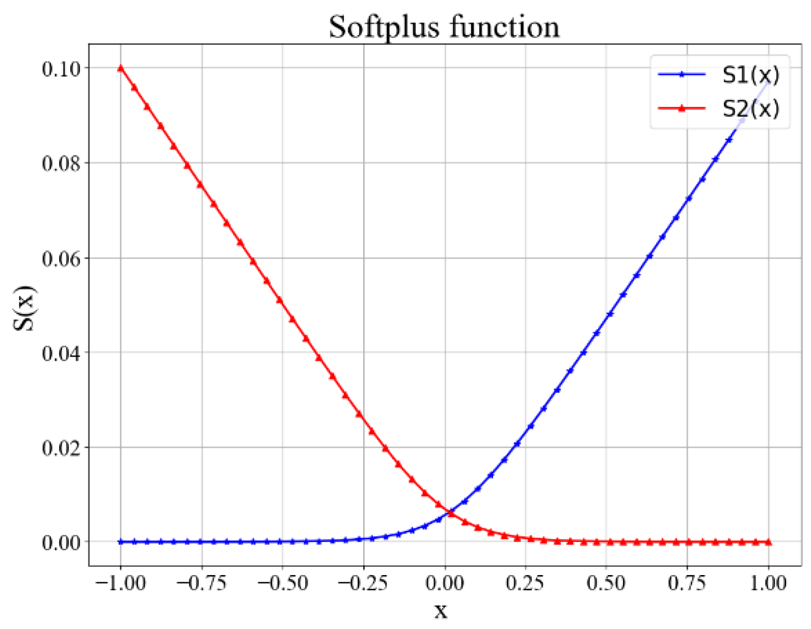
- Reverse joint loss
4. Results
4.1. Bone Proportion and Length Recovery
4.1.1. Bone Segment Proportions
4.1.2. Bone Segment Lengths
4.2. Classification of Body Orientation
4.3. Reverse Joint Correction
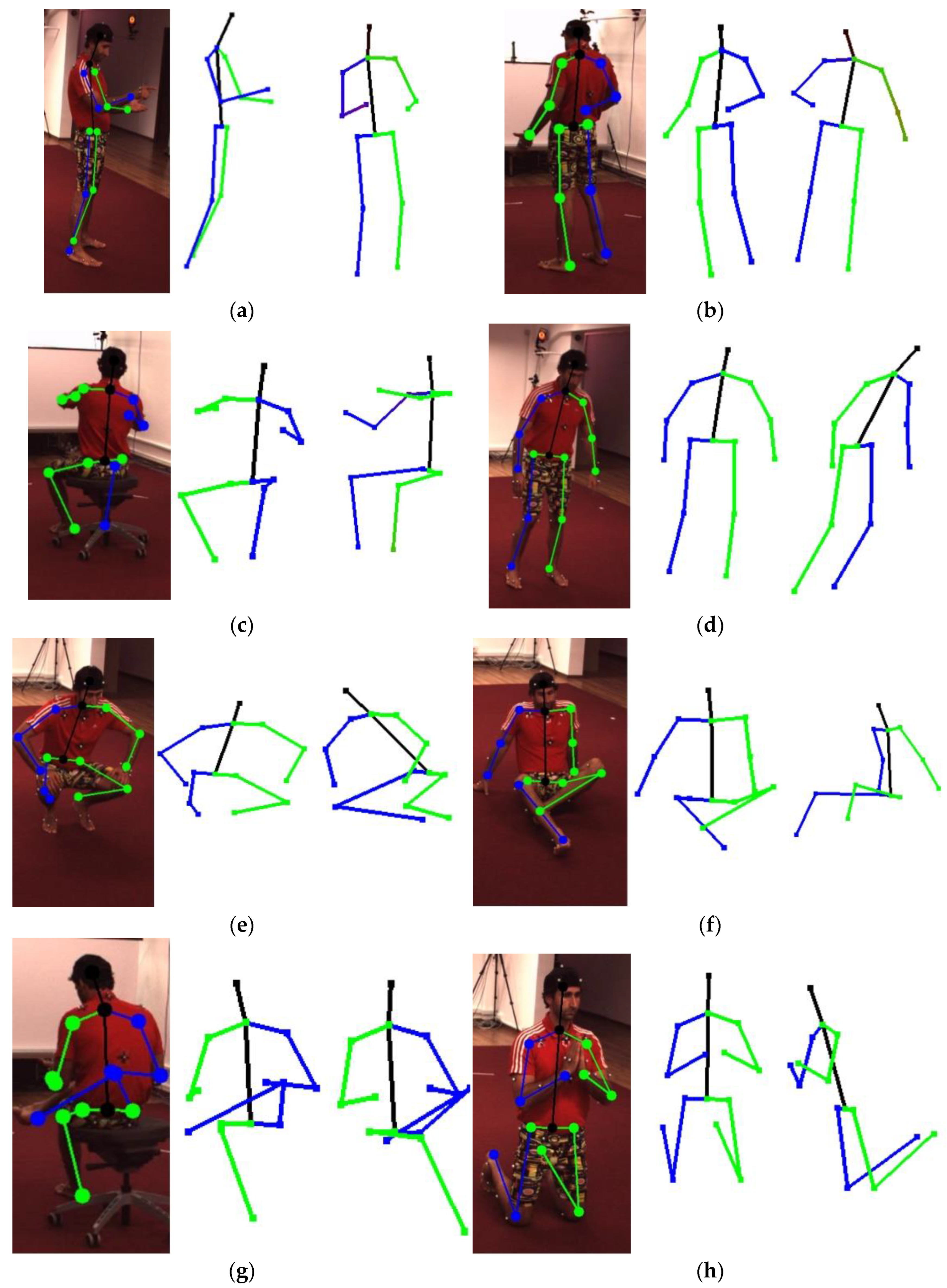
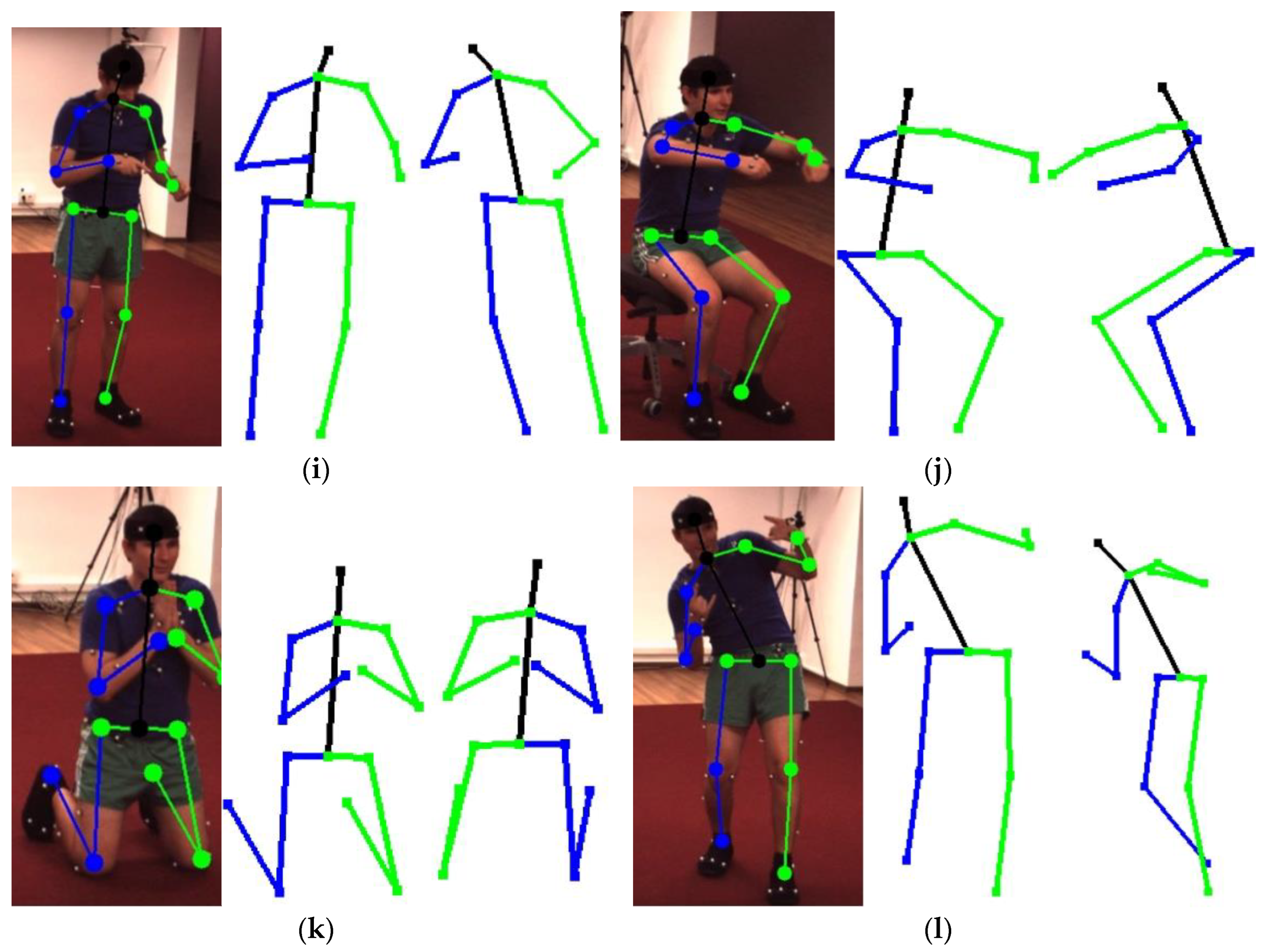
4.4. Three-Dimensional Human Pose Estimation Results
5. Discussions
5.1. Analysis about the Loss Functions
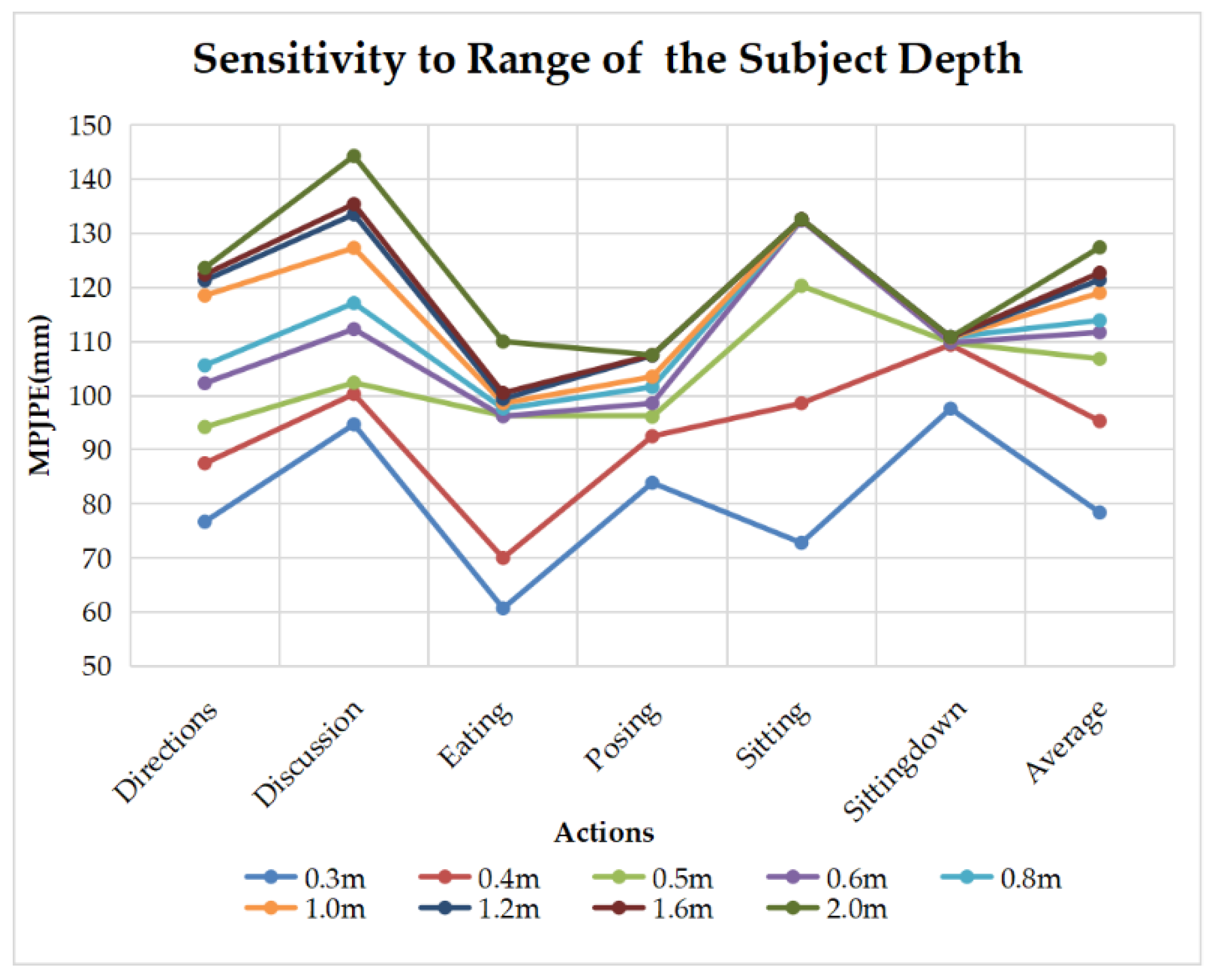
5.2. Sensitivity to the Depth Range of the Subject
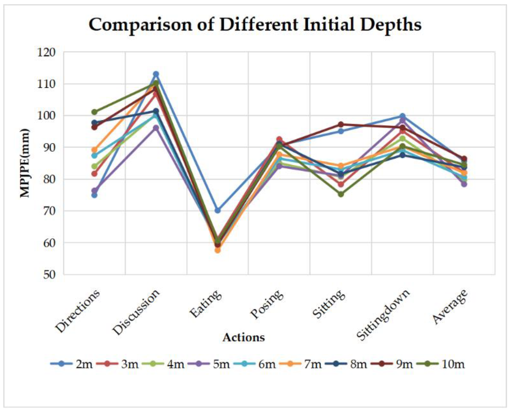
5.3. About the Initial Supposed Depth
6. Conclusions
Author Contributions
Funding
Institutional Review Board Statement
Informed Consent Statement
Data Availability Statement
Conflicts of Interest
References
- Liu, W.; Mei, T. Recent Advances of Monocular 2D and 3D Human Pose Estimation: A Deep Learning Perspective. ACM Comput. Surv. (CSUR) 2022. [Google Scholar] [CrossRef]
- Fang, H.S.; Cao, J.; Tai, Y.W.; Lu, C. Pairwise body-part attention for recognizing human-object interactions. In Proceedings of the European Conference on Computer Vision (ECCV), Munich, Germany, 8–14 September 2018; pp. 51–67. [Google Scholar]
- Chéron, G.; Laptev, I.; Schmid, C. P-cnn: Pose-based cnn features for action recognition. In Proceedings of the IEEE International Conference on Computer Vision, Santiago, Chile, 13–16 December 2015; pp. 3218–3226. [Google Scholar]
- Su, C.; Li, J.; Zhang, S.; Xing, J.; Gao, W.; Tian, Q. Pose-driven deep convolutional model for person re-identification. In Proceedings of the IEEE International Conference on Computer Vision, Venice, Italy, 22–29 October 2017; pp. 3960–3969. [Google Scholar]
- Zhou, X.; Zhu, M.; Pavlakos, G.; Leonardos, S.; Derpanis, K.G.; Daniilidis, K. Monocap: Monocular human motion capture using a cnn coupled with a geometric prior. IEEE Trans. Pattern Anal. Mach. Intell. 2018, 41, 901–914. [Google Scholar] [CrossRef] [PubMed]
- Fan, X.; Zheng, K.; Lin, Y.; Wang, S. Combining local appearance and holistic view: Dual-source deep neural networks for human pose estimation. In Proceedings of the IEEE Conference on Computer Vision and Pattern Recognition, Boston, MA, USA, 7–12 June 2015; pp. 1347–1355. [Google Scholar]
- Wei, S.E.; Ramakrishna, V.; Kanade, T.; Sheikh, Y. Convolutional pose machines. In Proceedings of the IEEE Conference on Computer Vision and Pattern Recognition, Las Vegas, NV, USA, 27–30 June 2016; pp. 4724–4732. [Google Scholar]
- Cao, Z.; Simon, T.; Wei, S.E.; Wei, S.; Sheikh, Y. Realtime multi-person 2d pose estimation using part affinity fields. In Proceedings of the IEEE Conference on Computer Vision and Pattern Recognition, Honolulu, HI, USA, 21–26 July 2017; pp. 7291–7299. [Google Scholar]
- Chen, Y.; Wang, Z.; Peng, Y.; Zhang, Z. Cascaded pyramid network for multi-person pose estimation. In Proceedings of the IEEE Conference on Computer Vision and Pattern Recognition, Salt Lake City, UT, USA, 18–22 June 2018; pp. 7103–7112. [Google Scholar]
- Sarafianos, N.; Boteanu, B.; Ionescu, B.; Kakadiari, I.A. 3d human pose estimation: A review of the literature and analysis of covariates. Comput. Vis. Image Underst. 2016, 152, 1–20. [Google Scholar] [CrossRef]
- Fischler, M.A.; Elschlager, R.A. The representation and matching of pictorial structures. IEEE Trans. Comput. 1973, 100, 67–92. [Google Scholar] [CrossRef]
- Zuffi, S.; Freifeld, O.; Black, M.J. From pictorial structures to deformable structures. In Proceedings of the 2012 IEEE Conference on Computer Vision and Pattern Recognition, Providence, RI, USA, 16–21 June 2012; pp. 3546–3553. [Google Scholar]
- Huang, J.B.; Yang, M.H. Estimating human pose from occluded images. In Proceedings of the Asian Conference on Computer Vision, Xi’an, China, 23–27 September 2009; Springer: Berlin/Heidelberg, Germany, 2009; pp. 48–60. [Google Scholar]
- Sigal, L.; Black, M.J. Guest editorial: State of the art in image-and video-based human pose and motion estimation. Int. J. Comput. Vis. 2010, 87, 1–4. [Google Scholar] [CrossRef]
- Okada, R.; Soatto, S. Relevant feature selection for human pose estimation and localization in cluttered images. In Proceedings of the European Conference on Computer Vision, Marseille, France, 12–18 October 2008; Springer: Berlin/Heidelberg, Germany, 2008; pp. 434–445. [Google Scholar]
- Jiang, H. 3d human pose reconstruction using millions of exemplars. In Proceedings of the 2010 20th International Conference on Pattern Recognition, Istanbul, Turkey, 23–26 August 2010; pp. 1674–1677. [Google Scholar]
- Urtasun, R.; Darrell, T. Sparse probabilistic regression for activity-independent human pose inference. In Proceedings of the 2008 IEEE Conference on Computer Vision and Pattern Recognition, Anchorage, AK, USA, 24–26 June 2008; pp. 1–8. [Google Scholar]
- Greif, T.; Lienhart, R.; Sengupta, D. Monocular 3D human pose estimation by classification. In Proceedings of the 2011 IEEE International Conference on Multimedia and Expo, Barcelona, Spain, 11–15 July 2011; pp. 1–6. [Google Scholar]
- Ramakrishna, V.; Kanade, T.; Sheikh, Y. Reconstructing 3d human pose from 2d image landmarks. In Proceedings of the European Conference on Computer Vision, Florence, Italy, 7–13 October 2012; Springer: Berlin/Heidelberg, Germany, 2012; pp. 573–586. [Google Scholar]
- Dai, Y.; Li, H.; He, M. A simple prior-free method for non-rigid structure-from-motion factorization. Int. J. Comput. Vis. 2014, 107, 101–122. [Google Scholar] [CrossRef]
- Zhou, X.; Zhu, M.; Leonardos, S.; Daniilidis, K. Sparse representation for 3D shape estimation: A convex relaxation approach. IEEE Trans. Pattern Anal. Mach. Intell. 2016, 39, 1648–1661. [Google Scholar] [CrossRef] [PubMed]
- Ionescu, C.; Papava, D.; Olaru, V.; Sminchisescu, C. Human3. 6m: Large scale datasets and predictive methods for 3d human sensing in natural environments. IEEE Trans. Pattern Anal. Mach. Intell. 2013, 36, 1325–1339. [Google Scholar] [CrossRef] [PubMed]
- Sedai, S.; Bennamoun, M.; Huynh, D.Q. Localized fusion of Shape and Appearance features for 3D Human Pose Estimation. In Proceedings of the BMVC, Aberystwyth, UK, 31 August–3 September 2010; pp. 1–10. [Google Scholar]
- Salzmann, M.; Urtasun, R. Combining discriminative and generative methods for 3d deformable surface and articulated pose reconstruction. In Proceedings of the 2010 IEEE Computer Society Conference on Computer Vision and Pattern Recognition, San Francisco, CA, USA, 13–18 June 2010; pp. 647–654. [Google Scholar]
- Sigal, L.; Balan, A.O.; Black, M.J. Humaneva: Synchronized video and motion capture dataset and baseline algorithm for evaluation of articulated human motion. Int. J. Comput. Vis. 2010, 87, 4–27. [Google Scholar] [CrossRef]
- Kanazawa, A.; Black, M.J.; Jacobs, D.W.; Malik, J. End-to-end recovery of human shape and pose. In Proceedings of the IEEE Conference on Computer Vision and Pattern Recognition, Salt Lake City, UT, USA, 18–22 June 2018; pp. 7122–7131. [Google Scholar]
- Sun, K.; Xiao, B.; Liu, D.; Wang, J. Deep high-resolution representation learning for human pose estimation. In Proceedings of the IEEE/CVF Conference on Computer Vision and Pattern Recognition, Long Beach, CA, USA, 15–20 June 2019; pp. 5693–5703. [Google Scholar]
- Zheng, C.; Zhu, S.; Mendieta, M.; Yang, T.; Chen, C. 3d human pose estimation with spatial and temporal transformers. In Proceedings of the IEEE/CVF International Conference on Computer Vision, Virtual Event, 11–17 October 2021; pp. 11656–11665. [Google Scholar]
- Shan, W.; Lu, H.; Wang, S.; Zhang, X.; Gao, W. Improving robustness and accuracy via relative information encoding in 3d human pose estimation. In Proceedings of the 29th ACM International Conference on Multimedia, Chengdu, China, 20–24 October 2021; pp. 3446–3454. [Google Scholar]
- Zhang, J.; Tu, Z.; Yang, J.; Chen, Y.; Yuan, J. MixSTE: Seq2seq Mixed Spatio-Temporal Encoder for 3D Human Pose Estimation in Video. In Proceedings of the IEEE/CVF Conference on Computer Vision and Pattern Recognition, New Orleans, LA, USA, 19–24 June 2022; pp. 13232–13242. [Google Scholar]
- Deng, Y. Research on 3D Human Pose Estimation Technology Based on Skeletal Model Constraints. Master’s Thesis, Army Engineering University of PLA, Nanjing, China, 2018. [Google Scholar]
- Mur-Artal, R.; Montiel, J.M.; Tardos, J.D. ORB-SLAM: A versatile and accurate monocular SLAM system. IEEE Trans. Robot. 2015, 31, 1147–1163. [Google Scholar] [CrossRef]
- Triggs, B.; McLauchlan, P.F.; Hartley, R.I.; Fitzgibbon, A. Bundle adjustment—A modern synthesis. In Proceedings of the International Workshop on Vision Algorithms, Corfu, Greece, 21–22 September 1999; Springer: Berlin/Heidelberg, Germany, 1999; pp. 298–372. [Google Scholar]
- Kümmerle, R.; Grisetti, G.; Strasdat, H.; Konoli, K. g2o: A general framework for graph optimization. In Proceedings of the 2011 IEEE International Conference on Robotics and Automation, Shanghai, China, 9–13 May 2011; pp. 3607–3613. [Google Scholar]
- Lourakis, M.I.A. A Brief Description of the Levenberg-Marquardt Algorithm Implementedby Levmar; Technical Report; Institute of Computer Science, Foundation for Research and Technology—Hellas: Heraklion, Greece, 2005. [Google Scholar]
- Gavin, H.P. The Levenberg-Marquardt algorithm for nonlinear least squares curve-fitting problems. Dep. Civ. Environ. Eng. 2019, 5, 1–19. [Google Scholar]
- Lourakis, M.L.A.; Argyros, A.A. Is Levenberg-Marquardt the Most Efficient Optimization Algorithm for Implementing Bundle Adjustment? In Proceedings of the 10th IEEE International Conference on Computer Vision (ICCV 2005), Beijing, China, 17–20 October 2005.
- Available online: https://www.opengl.org/ (accessed on 21 February 2022).


| Symbol | Start | End | Symbol | Start | End |
|---|---|---|---|---|---|
| neck | head | right knee | right ankle | ||
| right shoulder | right elbow | left hip | left knee | ||
| right elbow | right wrist | left knee | left ankle | ||
| left shoulder | left elbow | right hip | right knee | ||
| left elbow | left wrist |
| Subject | Average | |||||||
|---|---|---|---|---|---|---|---|---|
| GPR | 0.072 | 0.078 | 0.089 | 0.083 | 0.052 | 0.073 | 0.055 | 0.072 |
| ours | 0.027 | 0.038 | 0.035 | 0.038 | 0.018 | 0.023 | 0.045 | 0.032 |
| Subject | Average | |||||||
|---|---|---|---|---|---|---|---|---|
| GPR | 0.055 | 0.048 | 0.057 | 0.049 | 0.032 | 0.041 | 0.035 | 0.045 |
| ours | 0.013 | 0.011 | 0.009 | 0.017 | 0.010 | 0.008 | 0.012 | 0.012 |
| Subject | Average | |||||||
|---|---|---|---|---|---|---|---|---|
| CPN 2D | 10.1 | 6.0 | 6.7 | 7.3 | 7.1 | 10.2 | 12.3 | 8.5 |
| GT 2D | 4.8 | 2.6 | 3.8 | 4.5 | 3.7 | 5.1 | 5.7 | 4.3 |
| Left Leg | Right Leg | Neck | Left Arm | Right Arm | Average |
|---|---|---|---|---|---|
| 84.4% | 94.6% | 84.6% | 83.8% |
| Action | Directions | Discussion | Eating | Posing | Sitting |
|---|---|---|---|---|---|
| PMP [19] | 126.7 | 133.5 | 124.7 | 136.2 | 146.1 |
| NRSFM [20] | 136.5 | 139.6 | 134.3 | 157.2 | 181.7 |
| Convex [21] | 94.3 | 89.2 | 85.4 | 96.1 | 80.1 |
| Monocap [5] | 73.1 | 69.2 | 82.0 | 73.7 | 71.4 |
| Ours | 76.7 | 94.7 | 60.7 | 83.9 | 72.8 |
| Action | Sitting Down | Average | |||
| PMP [19] | 162.4 | 134.4 | |||
| NRSFM [20] | 176.9 | 150.7 | |||
| Convex [21] | 97.4 | 90.4 | |||
| Monocap [5] | 90.3 | 76.4 | |||
| Ours | 97.6 | 78.4 |
| Action | Directions | Discussion | Eating | Posing | Sitting | Sitting Down | Total |
|---|---|---|---|---|---|---|---|
| PMP [19] | 0.22 | 0.21 | 0.21 | 0.22 | 0.22 | 0.23 | 0.22 |
| NRSFM [20] | <0.1 | <0.1 | <0.1 | <0.1 | <0.1 | <0.1 | <0.1 |
| Convex [21] | 0.52 | 0.51 | 0.51 | 0.52 | 0.50 | 0.51 | 0.51 |
| Monocap [5] | 0.85 | 0.84 | 0.86 | 0.84 | 0.85 | 0.86 | 0.85 |
| Ours | 31.43 | 32.51 | 33.60 | 32.38 | 32.81 | 31.77 | 32.54 |
Publisher’s Note: MDPI stays neutral with regard to jurisdictional claims in published maps and institutional affiliations. |
© 2022 by the authors. Licensee MDPI, Basel, Switzerland. This article is an open access article distributed under the terms and conditions of the Creative Commons Attribution (CC BY) license (https://creativecommons.org/licenses/by/4.0/).
Share and Cite
Sun, H.; Zhang, Y.; Zheng, Y.; Luo, J.; Pan, Z. G2O-Pose: Real-Time Monocular 3D Human Pose Estimation Based on General Graph Optimization. Sensors 2022, 22, 8335. https://doi.org/10.3390/s22218335
Sun H, Zhang Y, Zheng Y, Luo J, Pan Z. G2O-Pose: Real-Time Monocular 3D Human Pose Estimation Based on General Graph Optimization. Sensors. 2022; 22(21):8335. https://doi.org/10.3390/s22218335
Chicago/Turabian StyleSun, Haixun, Yanyan Zhang, Yijie Zheng, Jianxin Luo, and Zhisong Pan. 2022. "G2O-Pose: Real-Time Monocular 3D Human Pose Estimation Based on General Graph Optimization" Sensors 22, no. 21: 8335. https://doi.org/10.3390/s22218335
APA StyleSun, H., Zhang, Y., Zheng, Y., Luo, J., & Pan, Z. (2022). G2O-Pose: Real-Time Monocular 3D Human Pose Estimation Based on General Graph Optimization. Sensors, 22(21), 8335. https://doi.org/10.3390/s22218335