

A Complement Method for Magnetic Data Based on TCN-SE Model


Abstract
1. Introduction
2. Data Description and Calibrating Installation Matrix
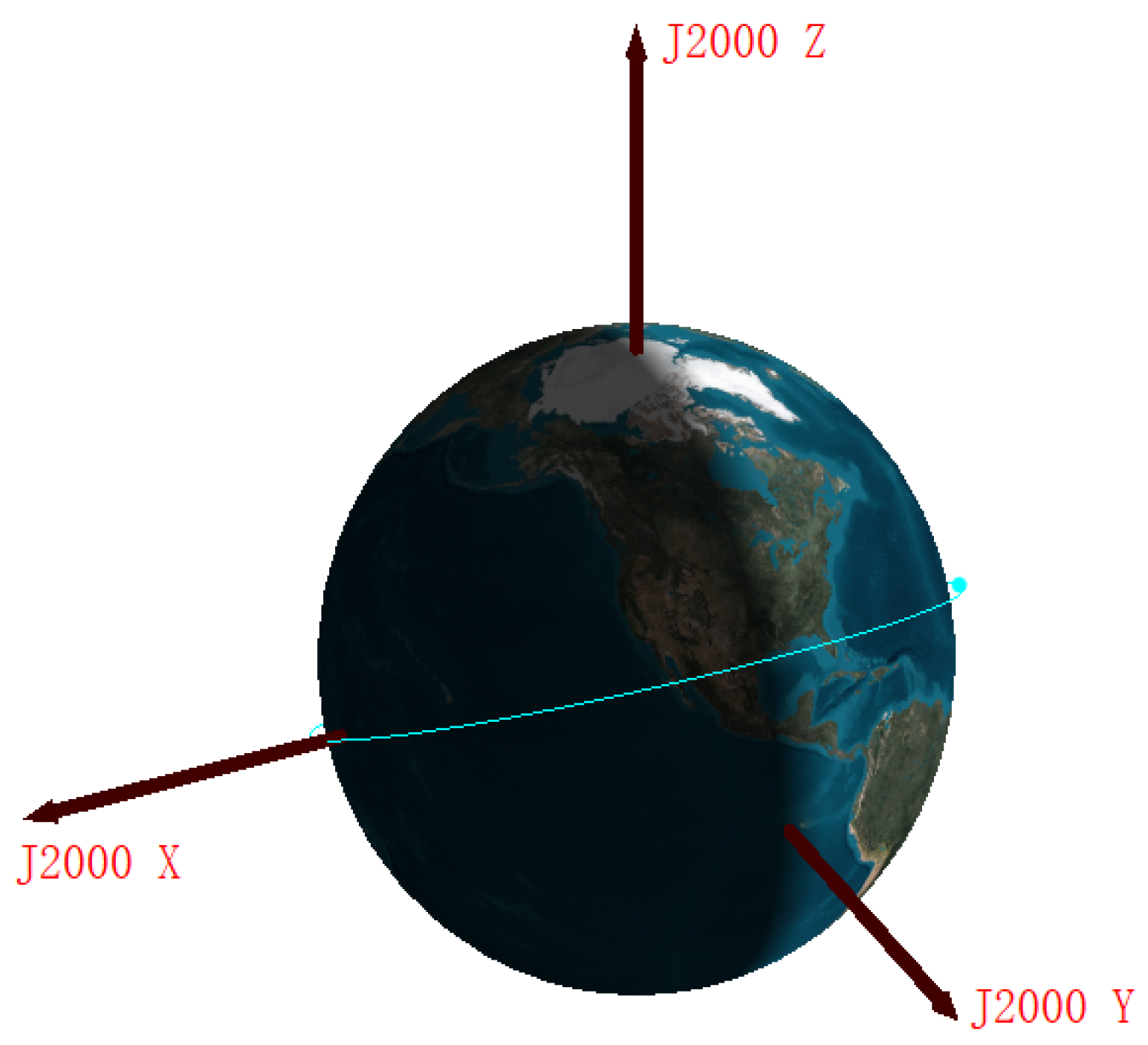
2.1. Coordinate Systems
- J2000 coordinate system: As shown in Figure 1, the origin is at the center of the Earth, the X axis points to the vernal equinox, the Y axis is in the equatorial plane and perpendicular to the X axis, and the Z axis points to the North Pole.
- Orbital coordinate system (VVLH): The origin of the orbital coordinate system is located at the satellite centroid, the Z axis points to the Earth center, the X axis is in the orbital plane and perpendicular to the Z axis, and the Y axis is determined by the right-hand rule.
- Body coordinate system: The origin of the body coordinate is located at the satellite’s center of mass, the X axis points to the satellite’s flight direction, the Z axis is in the satellite’s longitudinal symmetry plane, and the Y axis is perpendicular to the satellite’s longitudinal symmetry plane.
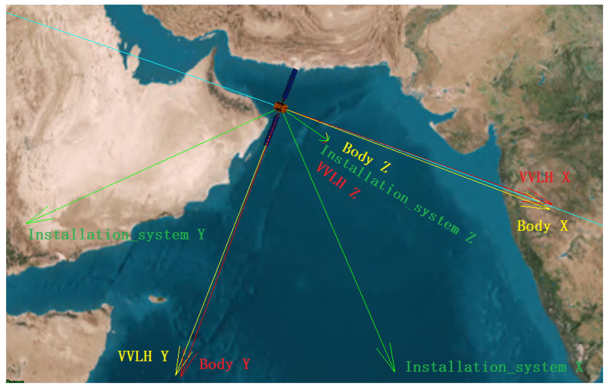
- Installation coordinate system: The installation position of the magnetometer varies from satellite to satellite. The three-axis installation coordinate system of the magnetometer is obtained by multiplying the body coordinate system by the installation matrix. The coordinate system is shown in Figure 2.
2.2. Geomagnetic Field Measurement
- Satellite body components: The current of solar panel, battery and magnetic torque, and hard and soft magnetic materials on the satellite generate magnetic fields [21]. These disturbances change with attitude, showing a time-related regularity. This part is the source of stray magnetism.
- External magnetic interference (not included in IGRF model): (1) The local anomaly of the lithosphere: it mainly comes from the short wavelength magnetic field caused by the geological characteristics of the Earth’s surface (mountains, oceans, minerals, etc.) [22]. (2) External field: the space current system above the Earth’s surface, which is mainly distributed in the ionosphere, that is, the upper atmosphere ionized by solar high-energy radiation and cosmic ray excitation [23]. The impact of this item can reach dozens of nT [24]. These two terms show periodic changes with orbital periods.
- IGRF fitting error. This part is minimal. Ref. [25] shows that the accuracy of the spherical harmonic coefficient of the eighth-order IGRF-11 is 0.1 nT.
- Effects of temperature change: (1) Uneven expansion of the satellite and the changes in the installation coordinate system, which has a slight impact. (2) Thermal drift, which is relatively large. Ref. [26] shows that the maximum drift of the magnetometer reaches 200 nT between 0 and 40 °C. This effect of temperature changes regularly with the satellite in the Earth’s shadow area or sunshine area.
2.3. Data Description
- Use the method in Algorithm 1 to detect abnormal sampling points:
- The outliers detected in step 1 are deleted, and then supplemented by our imputation method proposed in Figure 5.
| Algorithm 1: 3 outlier detection method |
 |
2.4. Calibration of Installation Matrix
- The three-axis magnetic vectors [, , ] are not related to each other;
- The [, , ] are independent and identically distributed;
- The three-axis vectors [, , ] are not related to the random term [, , ], that is, , , .
| Algorithm 2: The SGD algorithm (take the X axis as an example) |
 |
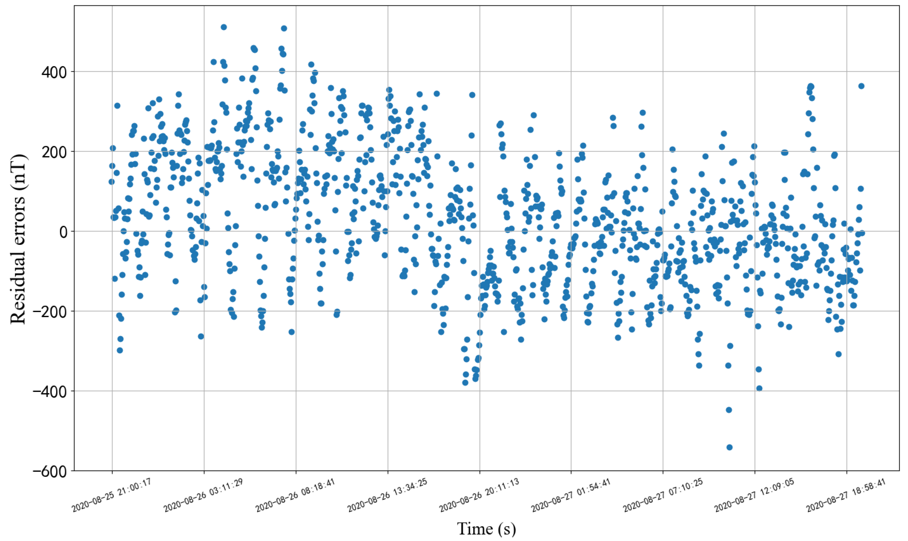
3. Processing of Residual Errors
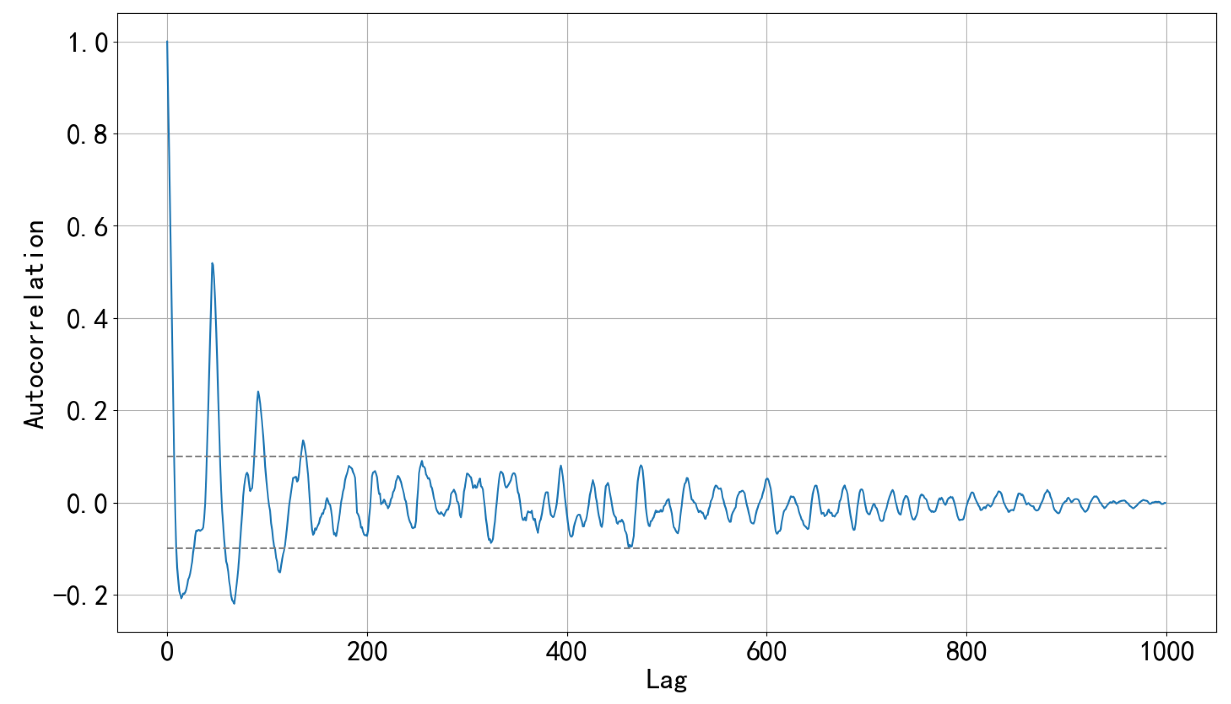
3.1. Autocorrelation of Residual Sequence
3.2. Time Series Model
3.2.1. TCN Network
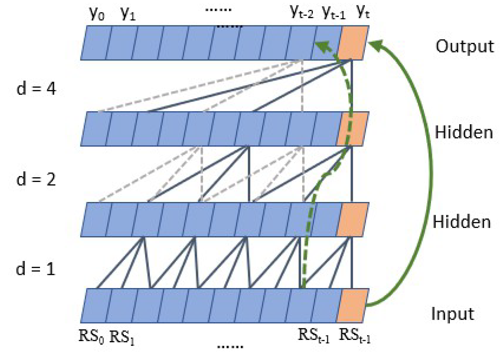
- Dilated Causal ConvolutionAs shown in Figure 8, TCN has the characteristics of both causal convolution and dilated convolution [30]. Formally, for one-dimensional input sequence and a filter , the convolution result is,where k is the convolution filter size, d represents the sampling interval (expansion coefficient), and accounts for the direction of the past. When , it indicates that each point is collected, and the higher the level, the larger the d.Causal convolution ensures that the output result at each time is determined by the current and previous time. The advantage of dilated convolution is that it increases the receptive fields without pooling loss information, so that each convolution output contains a large range of information. At the same time, the property of interval sampling avoids the problem of too many convolution layers and reduces the risk of gradient disappearance. Thus, it allows for both very deep networks and a very long effective history.
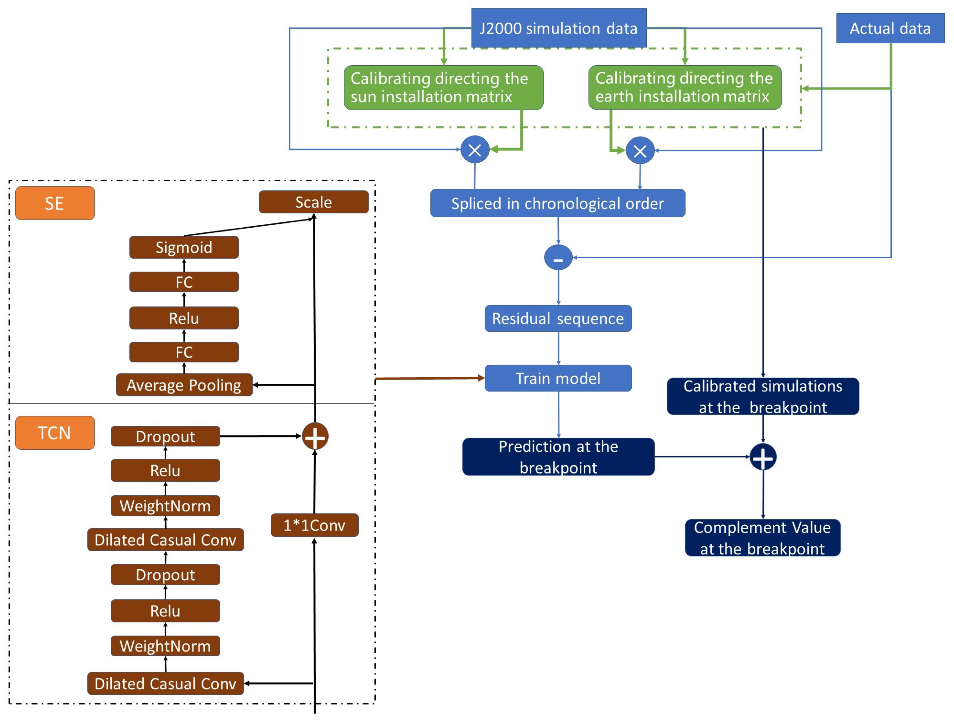
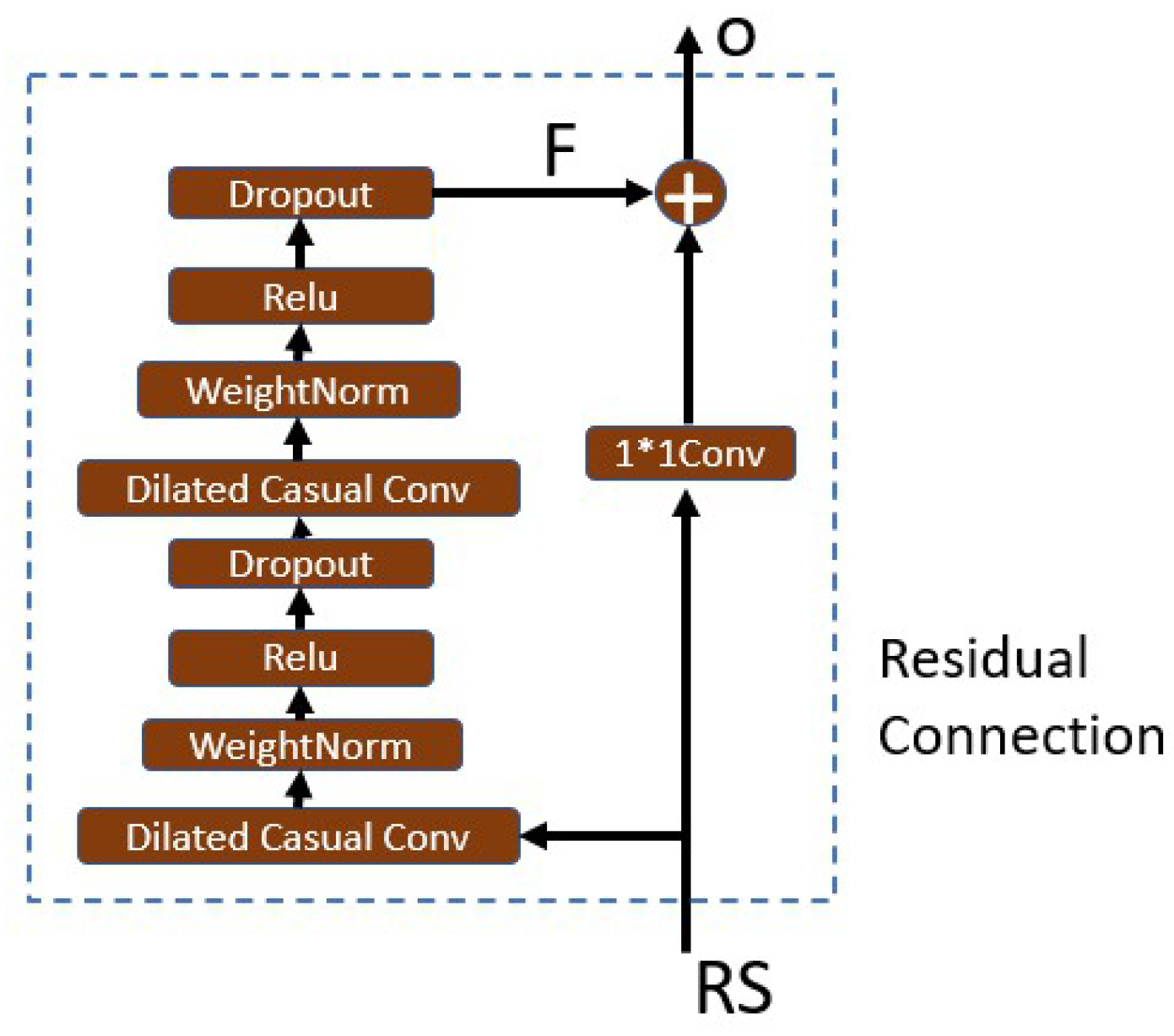
- Residual connectionResidual connection transmits information directly between layers without convolution, which is a very effective way to train deep networks [31]. Figure 9 shows that in a residual block, the signal is transmitted by a weight layer composed of a series of operations such as causal expansion convolution and normalization, and also is directly mapped to the sum of the output of the weight layer,where o is the output of the residual block. If , the block turns into an identity map, and thus degenerates into a shallow network. This structure has the advantages of both the depth of the deep network and the shallow network. At the same time, even if the gradient of the weight layer is 0, the gradient of the entire residual network can be guaranteed not to be 0 due to the existence of the direct mapping mechanism. This block reduces the risk of vanishing gradients further when the model depth increases.The advantages of the TCN can be analyzed as follows:
- In backpropagation, gradients do not accumulate along the time dimension, but along the network depth direction, and the number of network layers is often much smaller than the length of the input sequence. Furthermore, with the help of residual connection, the risk of gradient disappearance is further reduced, thus avoiding the gradient vanishing of RNN and LSTM networks.
- The TCN does not have to wait until the previous time is completed before calculating the result of the current time. Instead, all times are convoluted at the same time, which realizes parallelization and greatly reduces the running time.
- The dilated casual convolution mechanism of the TCN determines that it can use long-term historical information to predict by increasing the receptive field without dramatically increasing the model depth, which proves that it has the ability to remember long-term historical information.
In addition, in the copy memory task experiment [16], the TCN has no decline in memory ability in the sequence length from 0 to 250, and the 135 orders autocorrelation of our residual sequence is just in this range. - Formula of the TCN receptive fieldwhere represents the number of residual blocks in the TCN, and the sum of indicates how many causal convolution layers are stacked in each residual block. For example, indicates that four causal convolution layers are stacked, and the expansion factors of each convolution layer are 1, 2, 3, and 4, respectively.We determine the parameters of the TCN according to the above formula and Figure 8, the sequence has the maximum 135-order autocorrelation, so the input sequence length is set to 150; since the first five orders have significant autocorrelation (the autocorrelation coefficients are all greater than 0.5), the convolution kernel size is set to 6; the length of the input sequence is not too large, so the number of residual blocks is set to 2. This way the receptive field is larger than the length of the input sequence. According to Formula (6), the depth is set to 4, . The maximum missing points interval is 24, so the output length of the whole model is set to 30.
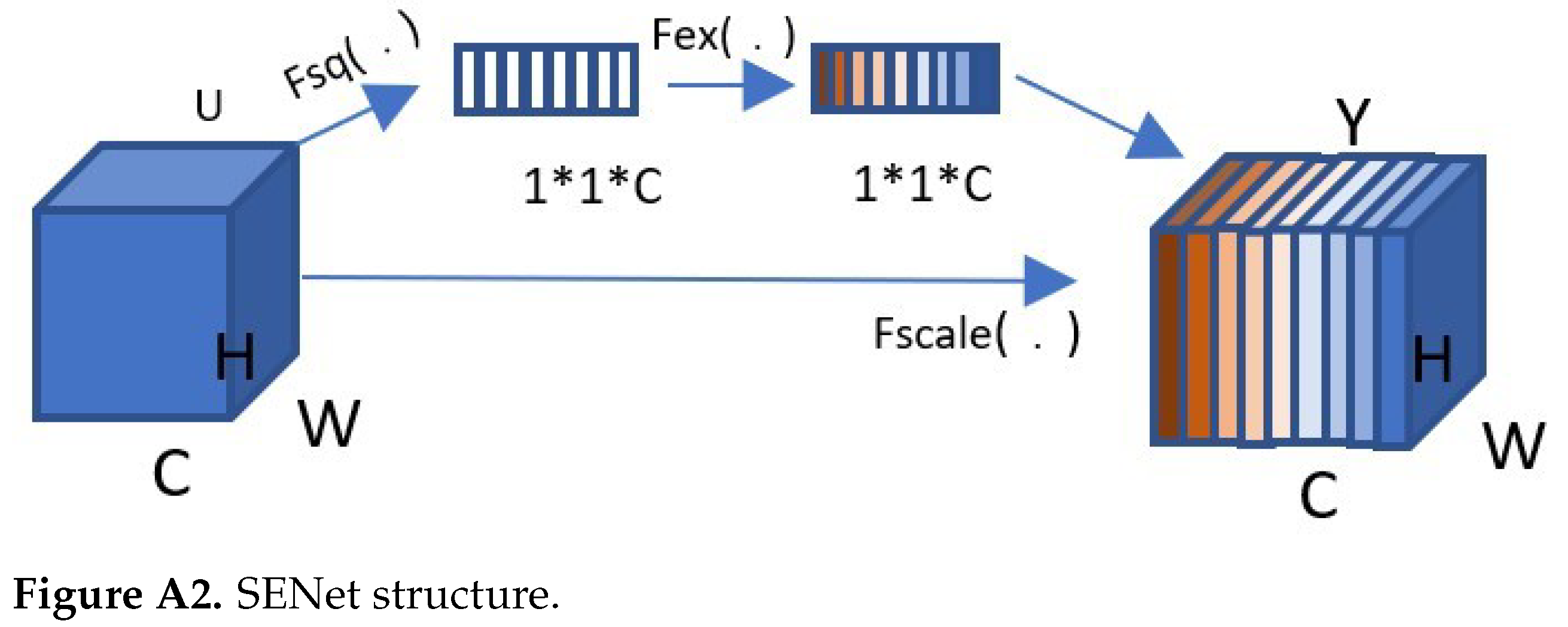
3.2.2. SE Attention Mechanism Module
4. The Overall Framework
5. Experiment and Result Analysis
5.1. Continuous Sequence
5.1.1. Data Acquisition
5.1.2. Model Evaluation Metrics
5.1.3. Deep Learning Experiment
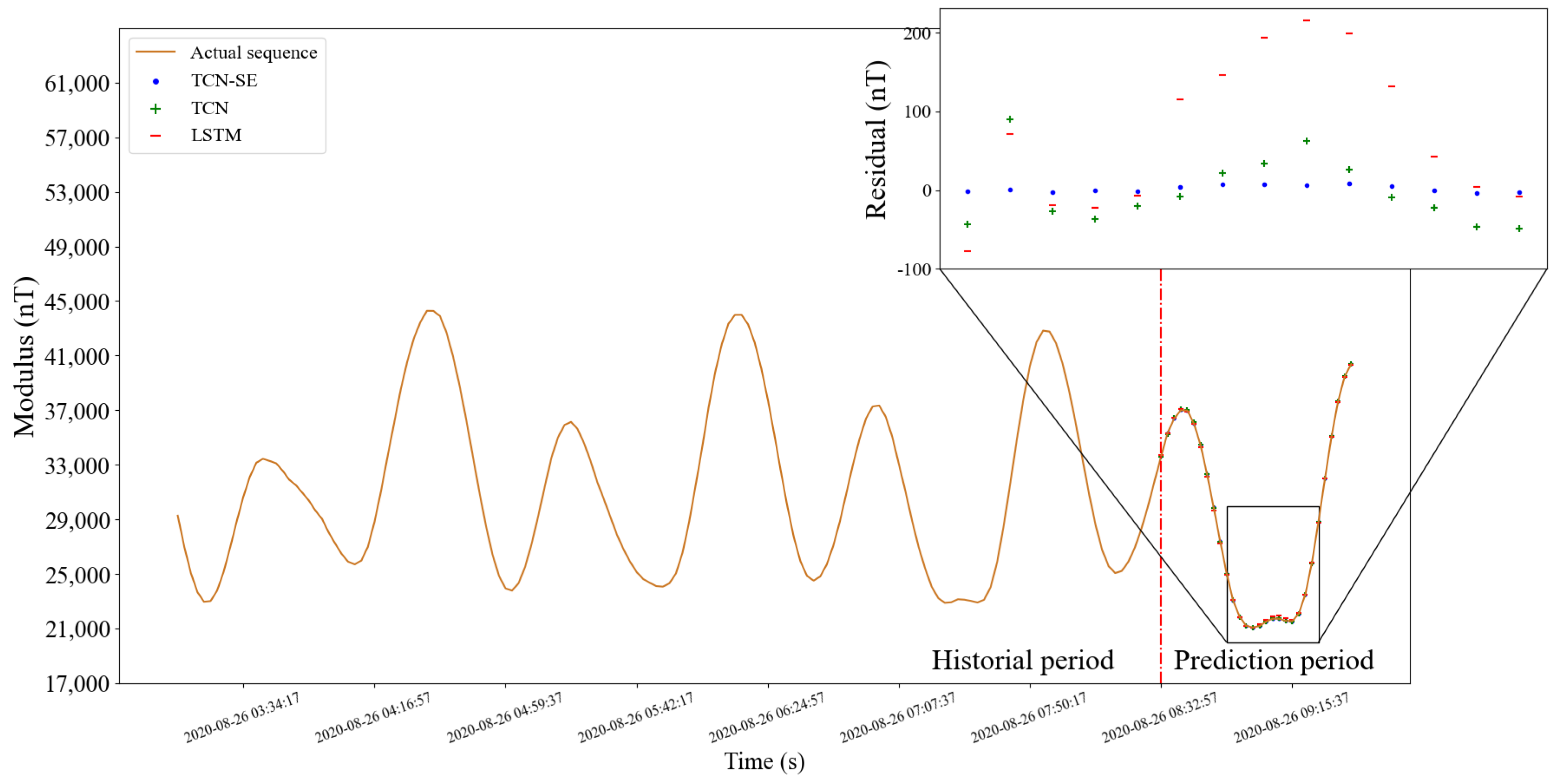
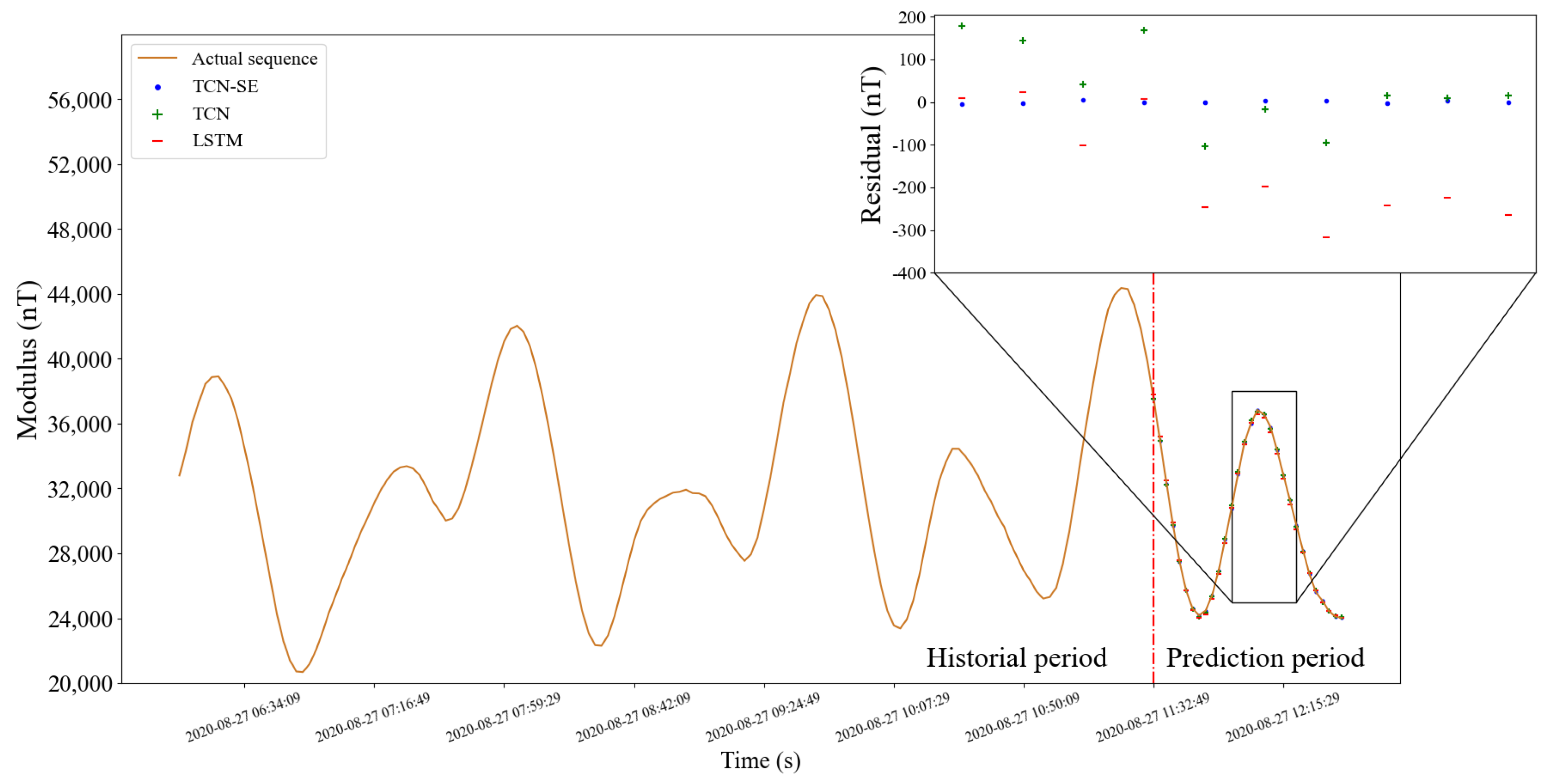
5.1.4. Comparison of Different Models
5.1.5. Prediction on Test Set
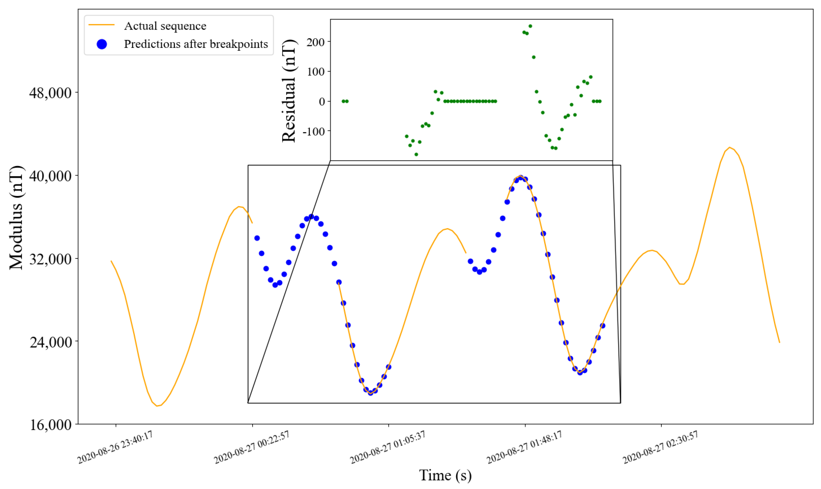
5.2. Sequence with Breakpoints
5.2.1. Data Acquisition
5.2.2. Model Evaluation Metrics
5.2.3. Comparison of Different Models
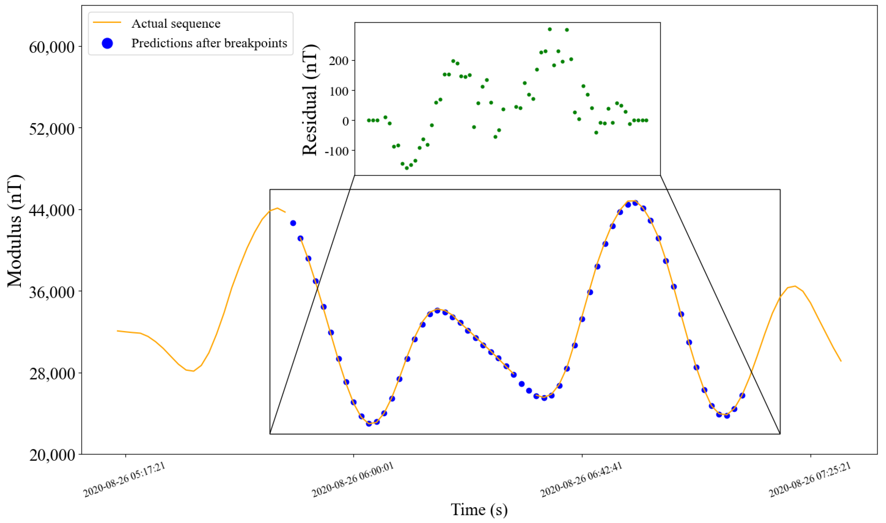
5.2.4. Prediction Effect
6. Conclusions
Author Contributions
Funding
Institutional Review Board Statement
Informed Consent Statement
Data Availability Statement
Conflicts of Interest
Appendix A. Discussion of LSTM Disadvantages
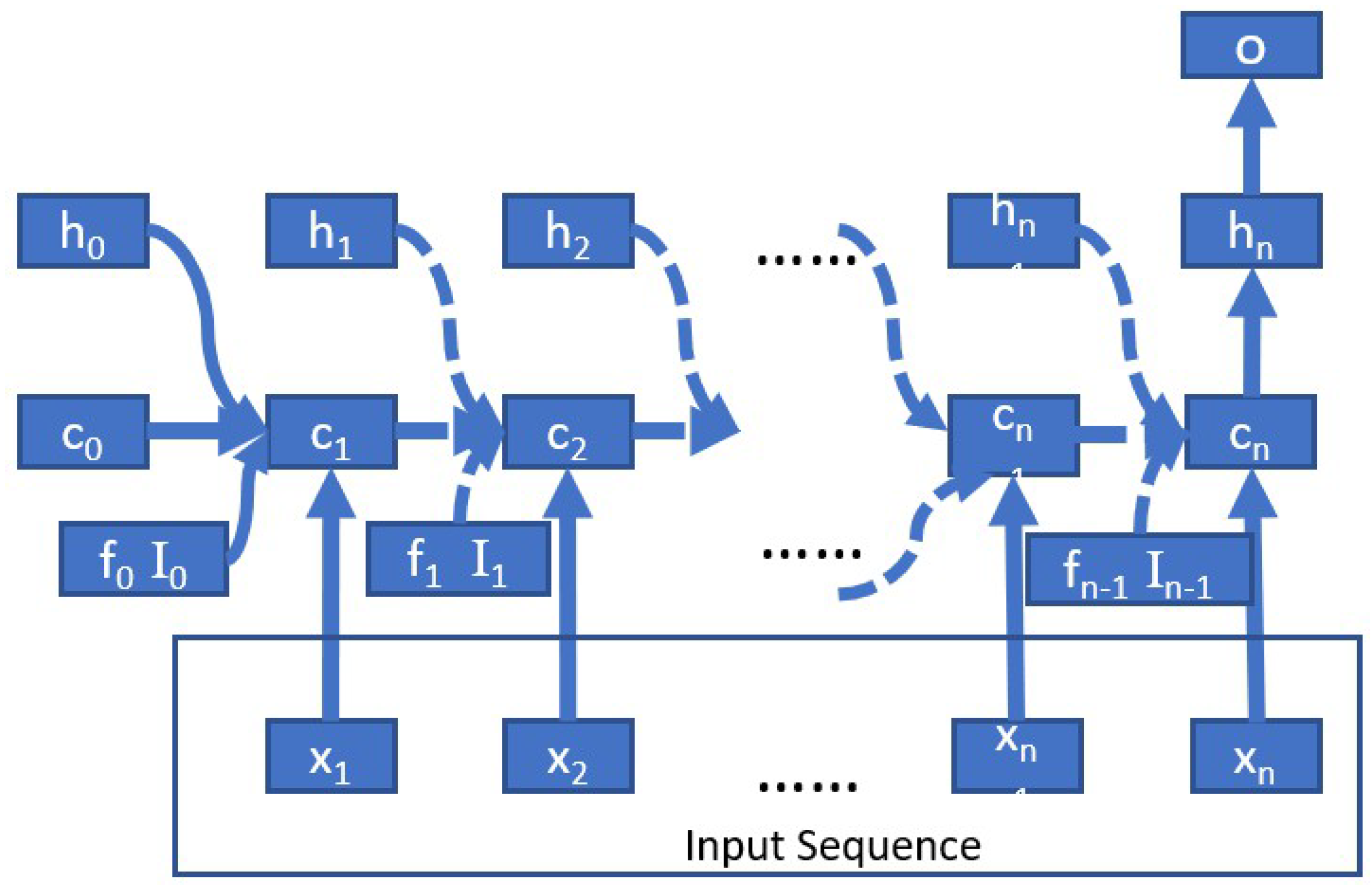
- LSTM cannot completely eliminate the risk of gradient descent in a long sequence and may cause gradient explosion.We use the simplified version of the LSTM block diagram shown in Figure A1 to illustrate this problem. For the parameter , the gradient formula for reverse conduction is:

- 2.
- Each LSTM unit has four full connection layers. If the time span is long, the network will be deep, and calculations will be cumbersome and time-consuming.
Appendix B. SE attention mechanism
Appendix B.1. Squeeze and Excitation

References
- Gao, D.; Zhang, T.; Cui, F.; Li, M. Development of Geomagnetic Navigation and Study of High Precision Geomagnetic Navigation for LEO Satellites. In Proceedings of the Second China Aerospace Safety Conference, Brussels, Belgium, 14–16 June 2017; pp. 438–445. [Google Scholar]
- Macmillan, S.; Finlay, C. The international geomagnetic reference field. In Geomagnetic Observations and Models; Springer: Berlin/Heidelberg, Germany, 2011; pp. 265–276. [Google Scholar]
- Lippi, M.; Bertini, M.; Frasconi, P. Short-term traffic flow forecasting: An experimental comparison of time-series analysis and supervised learning. IEEE Trans. Intell. Transp. Syst. 2013, 14, 871–882. [Google Scholar] [CrossRef]
- Zhu, M. A Study on SVM Algorithm for Missing Data Processing. Master’s Thesis, Tianjin University, Tianjin, China, 2017. [Google Scholar]
- Gao, W.; Niu, K.; Cui, J.; Gao, Q. In A data prediction algorithm based on BP neural network in telecom industry. In Proceedings of the 2011 International Conference on Computer Science and Service System (CSSS), Nanjing, China, 27–29 June 2011; pp. 9–12. [Google Scholar]
- Li, L.; Li, Y.; Li, Z. Efficient missing data imputing for traffic flow by considering temporal and spatial dependence. Transp. Res. Part Emerg. Technol. 2013, 34, 108–120. [Google Scholar] [CrossRef]
- Alsharif, M.H.; Younes, M.K.; Kim, J. Time series ARIMA model for prediction of daily and monthly average global solar radiation: The case study of Seoul, South Korea. Symmetry 2019, 11, 240. [Google Scholar] [CrossRef]
- Rahman, M.A.; Yunsheng, L.; Sultana, N. Analysis and prediction of rainfall trends over Bangladesh using Mann–Kendall, Spearman’s rho tests and ARIMA model. Meteorol. Atmos. Phys. 2017, 129, 409–424. [Google Scholar] [CrossRef]
- Wu, X.; Wang, Y. Extended and Unscented Kalman filtering based feedforward neural networks for time series prediction. Appl. Math. Model. 2012, 36, 1123–1131. [Google Scholar] [CrossRef]
- Xiu, C.; Ren, X.; Li, Y.; Liu, M. Short-Term Prediction Method of Wind Speed Series Based on Kalman Filtering Fusion. Trans. China Electrotech. Soc. 2014, 29, 253–259. [Google Scholar]
- Zeng, J.; Qiao, W. Short-term solar power prediction using a support vector machine. Renew. Energy 2013, 52, 118–127. [Google Scholar] [CrossRef]
- De Brabanter, K.; De Brabanter, J.; Suykens, J.A.; De Moor, B. Approximate confidence and prediction intervals for least squares support vector regression. IEEE Trans. Neural Netw. 2010, 22, 110–120. [Google Scholar] [CrossRef]
- Tokgoz, A.; Unal, G. In A RNN based time series approach for forecasting turkish electricity load. In Proceedings of the 2018 26th Signal Processing and Communications Applications Conference (SIU), Izmir, Turkey, 2–5 May 2018; pp. 1–4. [Google Scholar]
- Hundman, K.; Constantinou, V.; Laporte, C.; Colwell, I.; Soderstrom, T. In Detecting spacecraft anomalies using lstms and nonparametric dynamic thresholding. In Proceedings of the 24th ACM SIGKDD International Conference on Knowledge Discovery & Data Mining, London, UK, 19–23 August 2018; pp. 387–395. [Google Scholar]
- Jian, X.; Gu, H.; Wang, R. A short-term photovoltaic power prediction method based on dual-channel CNN and LSTM. Electr. Power Sci. Eng. 2019, 35, 7–11. [Google Scholar]
- Bai, S.; Kolter, J.Z.; Koltun, V. An empirical evaluation of generic convolutional and recurrent networks for sequence modeling. arXiv 2018, arXiv:1803.01271. [Google Scholar]
- Oord, A.v.d.; Dieleman, S.; Zen, H.; Simonyan, K.; Vinyals, O.; Graves, A.; Kalchbrenner, N.; Senior, A.; Kavukcuoglu, K. Wavenet: A generative model for raw audio. arXiv 2016, arXiv:1609.03499. [Google Scholar]
- Dauphin, Y.N.; Fan, A.; Auli, M.; Grangier, D. In Language modeling with gated convolutional networks. In Proceedings of the International Conference on Machine Learning, Sydney, Australia, 6–11 August 2017; pp. 933–941. [Google Scholar]
- Gehring, J.; Auli, M.; Grangier, D.; Yarats, D.; Dauphin, Y.N. In Convolutional sequence to sequence learning. In Proceedings of the International Conference on Machine Learning, Sydney, Australia, 6–11 August 2017; pp. 1243–1252. [Google Scholar]
- Shi, C.; Zhang, R.; Yu, Y.; Sun, X.; Lin, X. A SLIC-DBSCAN Based Algorithm for Extracting Effective Sky Region from a Single Star Image. Sensors 2021, 21, 5786. [Google Scholar] [CrossRef] [PubMed]
- Olsen, N.; Albini, G.; Bouffard, J.; Parrinello, T.; Tøffner-Clausen, L.J.E. Magnetic observations from CryoSat-2: Calibration and processing of satellite platform magnetometer data. Earth Planets Space 2020, 72, 1–18. [Google Scholar] [CrossRef]
- Liu, Y.; Wang, S.; Zhang, J.; Zheng, Y.; Qiao, Y. Research on the eleventh generation IGRF. Acta Seismol. Sin. 2017, 35, 125–134. [Google Scholar]
- Yan, F.; Zhen-Chang, A.; Han, S.; Fei, M.J. Analysis of variation in geomagnetic field of Chinese mainland based on comprehensive model CM4. Acta Phys. Sin. 2010, 59, 8941–8953. [Google Scholar]
- Wang, D.J. Analysis of the international geomagnetic reference field error in the China continent. Chin. J. Geophys. 2003, 171–174. [Google Scholar]
- Chen, B.; Gu, Z.W.; Gao, J.T.; Yuan, J.H.; Di, C.Z. Geomagnetic secular variation in China during 2005–2010 described by IGRF-11 and its error analysis. Prog. Geophys. 2012, 27, 512–521. [Google Scholar]
- Pang, H.; Chen, D.; Pan, M.; Luo, S.; Zhang, Q.; Luo, F.J. Nonlinear temperature compensation of fluxgate magnetometers with a least-squares support vector machine. Meas. Sci. Technol. 2012, 23, 025008. [Google Scholar] [CrossRef]
- Shorshi, G.; Bar-Itzhack, I.Y. Satellite autonomous navigation based on magnetic field measurements. J. Guid. Control. Dyn. 1995, 18, 843–850. [Google Scholar] [CrossRef]
- Zhang, Y.; Xiong, R.; He, H.; Pecht, M. Long short-term memory recurrent neural network for remaining useful life prediction of lithiumion batteries. IEEE Trans. Veh. Technol. 2018, 67, 5695–5705. [Google Scholar] [CrossRef]
- Peng, L.; Liu, S.; Liu, R.; Wang, L. Effective long short-term memory with differ- ential evolution algorithm for electricity price prediction. Energy 2018, 162, 1301–1314. [Google Scholar] [CrossRef]
- Lea, C.; Flynn, M.D.; Vidal, R.; Reiter, A.; Hager, G.D. In Temporal convolutional networks for action segmentation and detection. In Proceedings of the IEEE Conference on Computer Vision and Pattern Recognition, Honolulu, HI, USA, 21–26 July 2017; pp. 156–165. [Google Scholar]
- He, K.; Zhang, X.; Ren, S.; Sun, J. In Deep residual learning for image recognition. In Proceedings of the IEEE Conference on Computer Vision and Pattern Recognition, Las Vegas, NV, USA, 27–30 June 2016; pp. 770–778. [Google Scholar]
- Komolkin, A.V.; Kupriyanov, P.; Chudin, A.; Bojarinova, J.; Kavokin, K.; Chernetsov, N.J. Theoretically possible spatial accuracy of geomagnetic maps used by migrating animals. J. R. Soc. Interface 2017, 14, 20161002. [Google Scholar] [CrossRef] [PubMed]
- Zhao, J.; Huang, F.; Lv, J.; Duan, Y.; Qin, Z.; Li, G. Do rnn and lstm have long memory? In Proceedings of the International Conference on Machine Learning, Virtual, 13–18 July 2020; pp. 11365–11375. [Google Scholar]


| Parameter | Settings |
|---|---|
| Number of residual blocks | 2 |
| Convolution kernel size | 6 |
| Dilations | [1, 2, 4, 8] |
| Model input length | 150 |
| Model output length | 30 |
| Number of iterations | 100 |
| Batch size | 16 |
| Loss function | MSE |
| Optimizer | Adam |
| Network | MAE (nT) | Error Range (nT) | Time Cost (s) |
|---|---|---|---|
| LSTM | 112.39 | (−446.24, 411.46) | 545 |
| TCN | 67.27 | (−225.98, 213.26) | 176 |
| TCN-SE | 55.71 | (−175.18, 168.28) | 251 |
| Network | MAE (nT) | Error Range (nT) |
|---|---|---|
| LSTM | 144.15 | (−483.42, 442.98) |
| TCN | 92.19 | (−254.67, 259.26) |
| TCN-SE | 74.63 | (−215.18, 211.63) |
Publisher’s Note: MDPI stays neutral with regard to jurisdictional claims in published maps and institutional affiliations. |
© 2022 by the authors. Licensee MDPI, Basel, Switzerland. This article is an open access article distributed under the terms and conditions of the Creative Commons Attribution (CC BY) license (https://creativecommons.org/licenses/by/4.0/).
Share and Cite
Chen, W.; Zhang, R.; Shi, C.; Zhu, Y.; Lin, X. A Complement Method for Magnetic Data Based on TCN-SE Model. Sensors 2022, 22, 8277. https://doi.org/10.3390/s22218277
Chen W, Zhang R, Shi C, Zhu Y, Lin X. A Complement Method for Magnetic Data Based on TCN-SE Model. Sensors. 2022; 22(21):8277. https://doi.org/10.3390/s22218277
Chicago/Turabian StyleChen, Wenqing, Rui Zhang, Chenguang Shi, Ye Zhu, and Xiaodong Lin. 2022. "A Complement Method for Magnetic Data Based on TCN-SE Model" Sensors 22, no. 21: 8277. https://doi.org/10.3390/s22218277
APA StyleChen, W., Zhang, R., Shi, C., Zhu, Y., & Lin, X. (2022). A Complement Method for Magnetic Data Based on TCN-SE Model. Sensors, 22(21), 8277. https://doi.org/10.3390/s22218277