

Adaptive Discount Factor for Deep Reinforcement Learning in Continuing Tasks with Uncertainty


Abstract
:1. Introduction
2. Related Work
3. Discount Factor in Reinforcement Learning
3.1. Reinforcement Learning
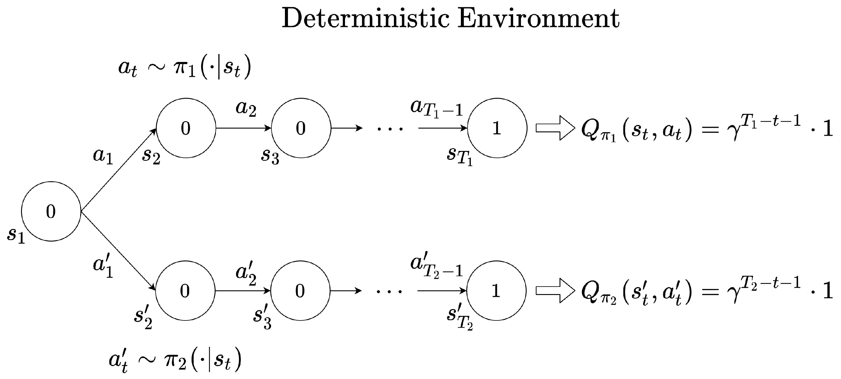
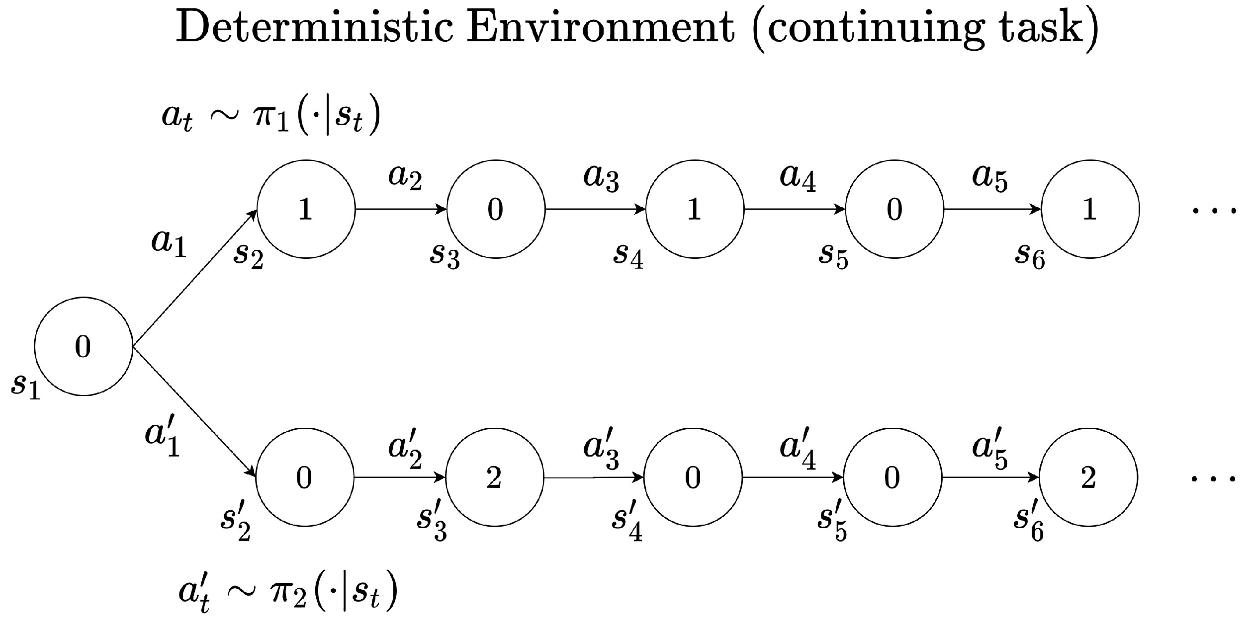
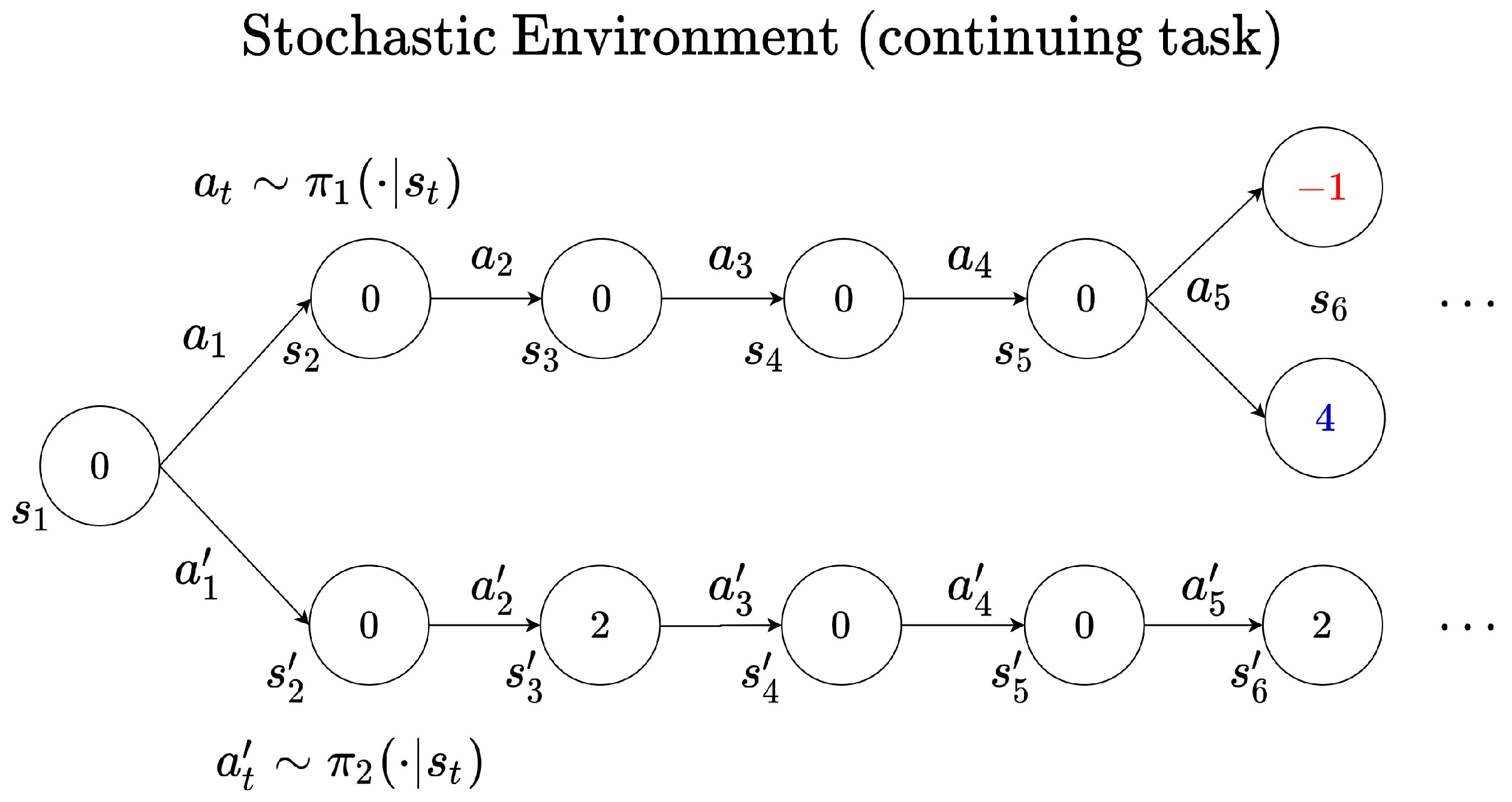
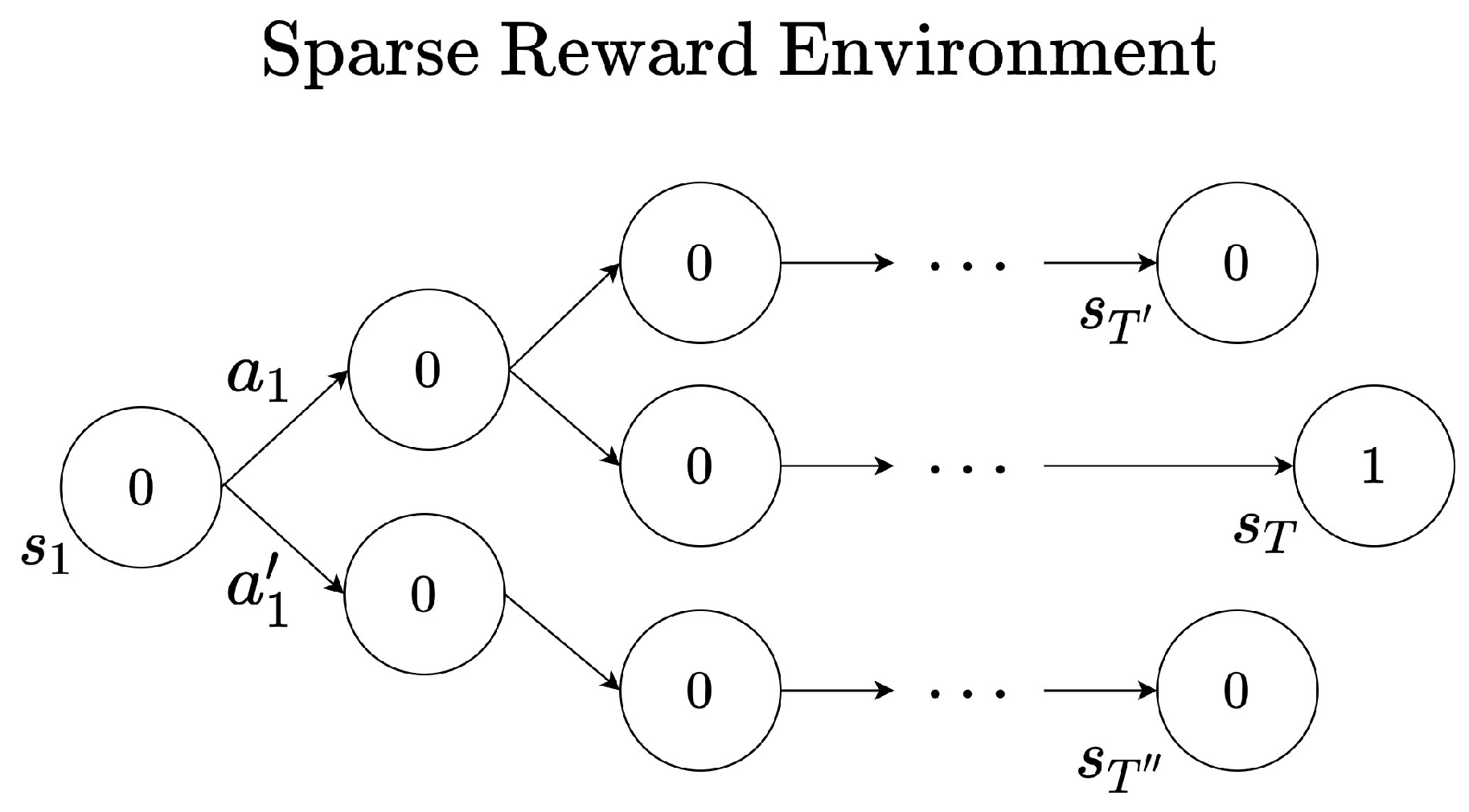
3.2. Role of the Discount Factor in Reinforcement Learning
4. Adaptive Discount Factor in Reinforcement Learning
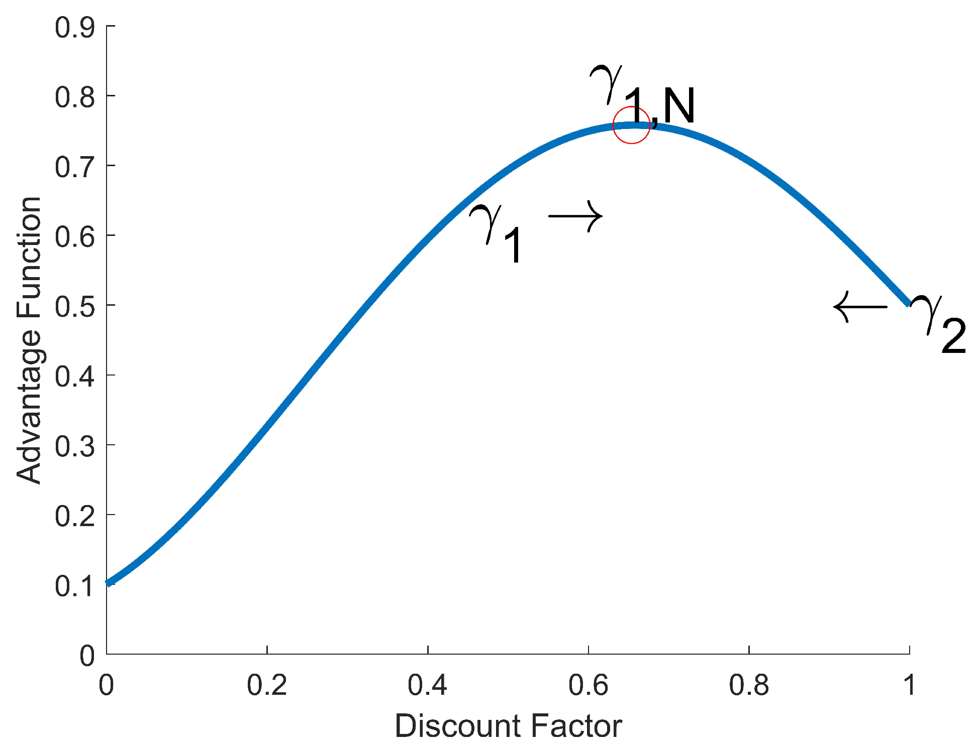
4.1. Adaptive Discount Factor
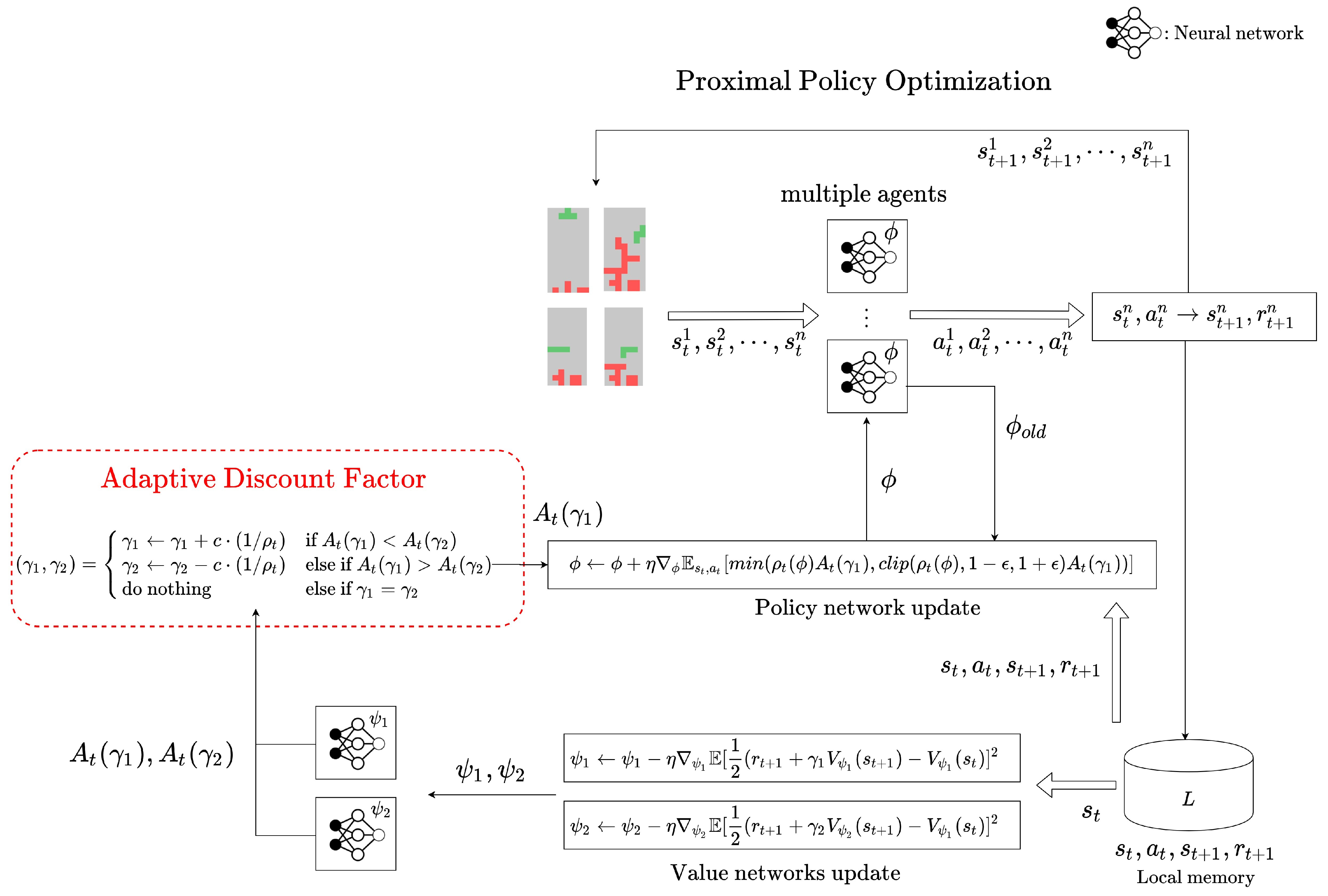
4.2. Adaptive Discount Factor in On-Policy RL
4.3. Adaptive Discount Factor in Off-Policy RL
5. Experiment in the Environments with Uncertainty
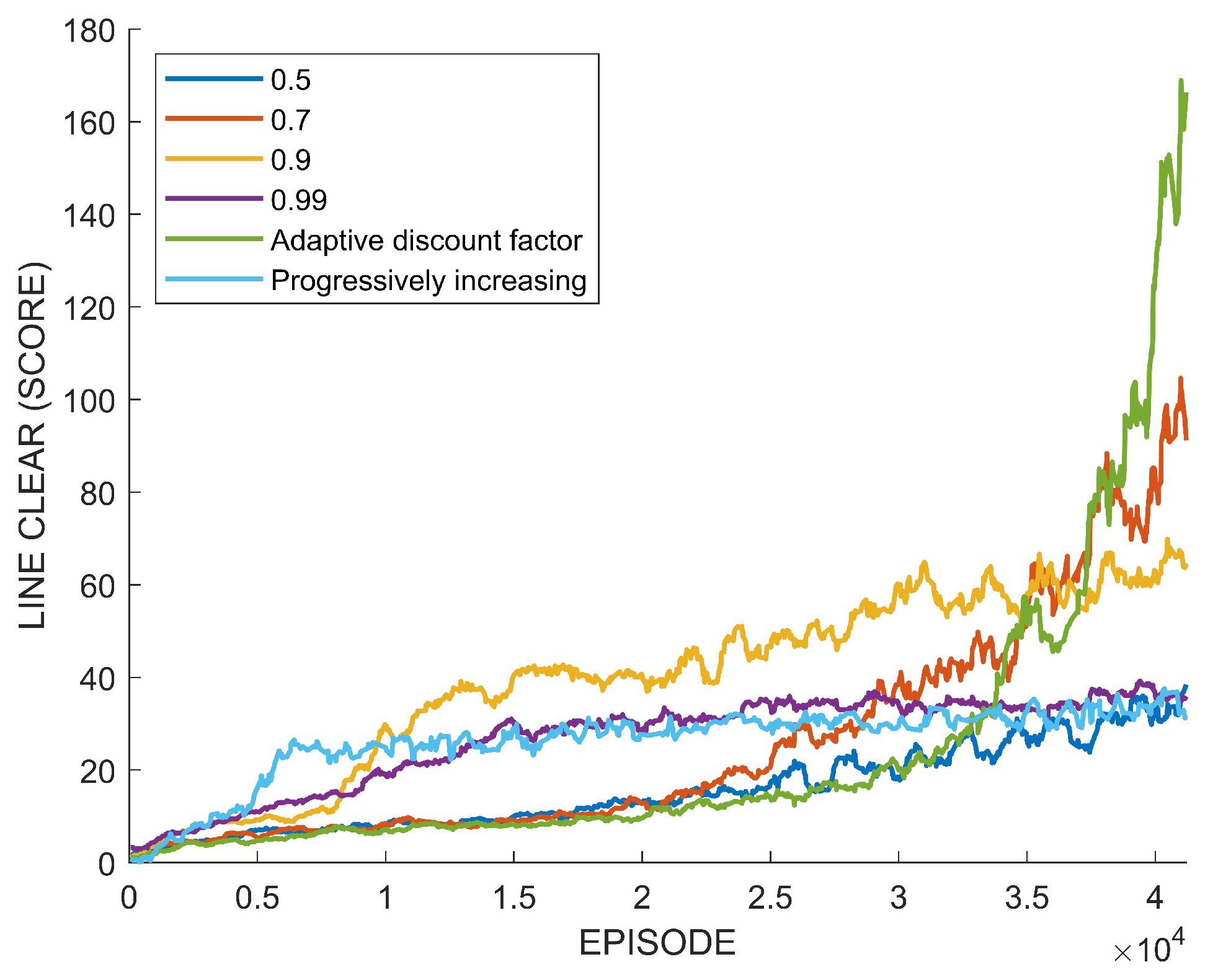
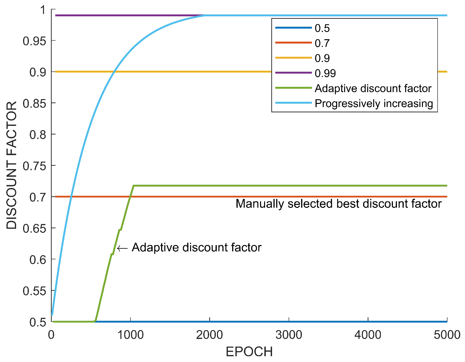
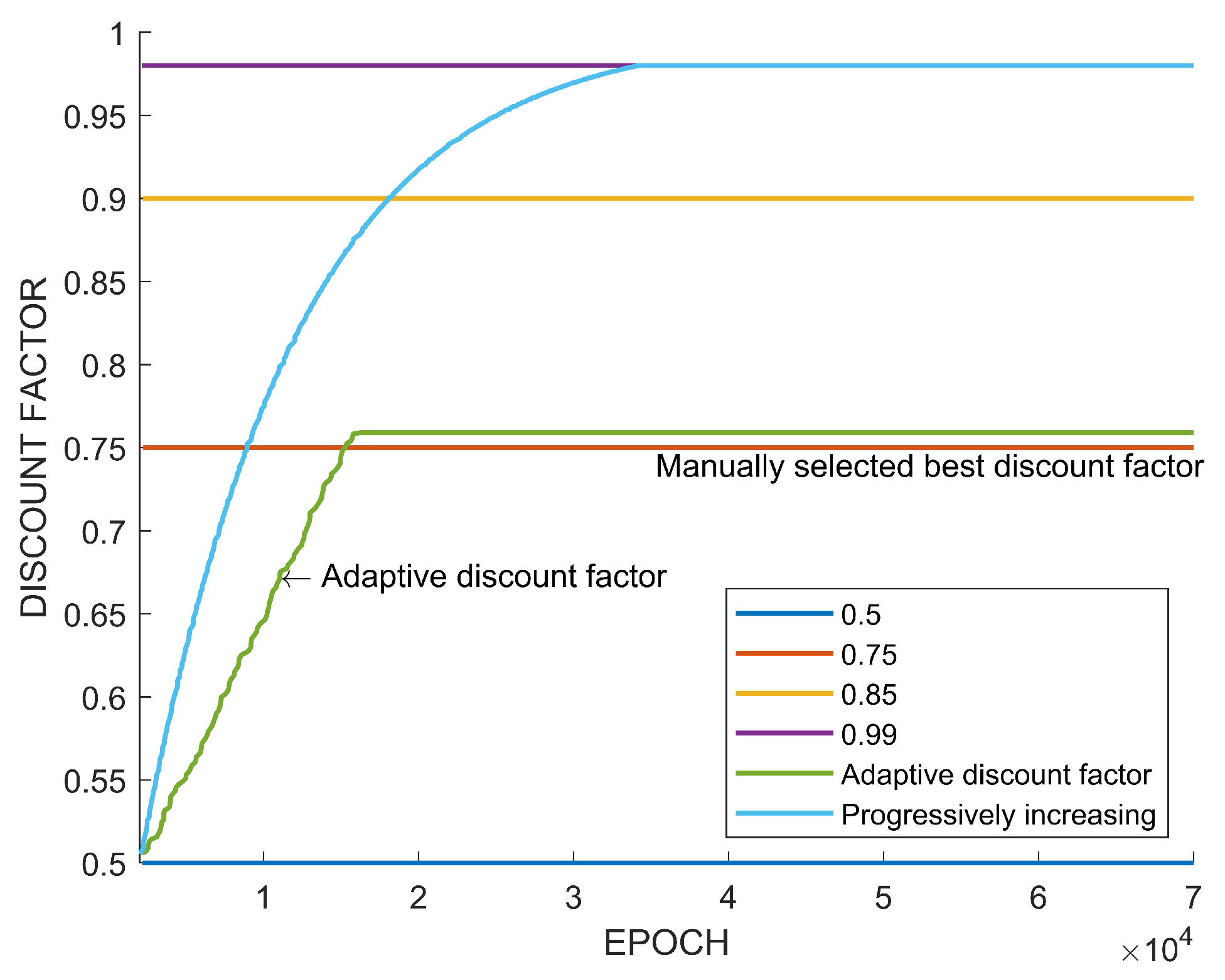
5.1. Tetris
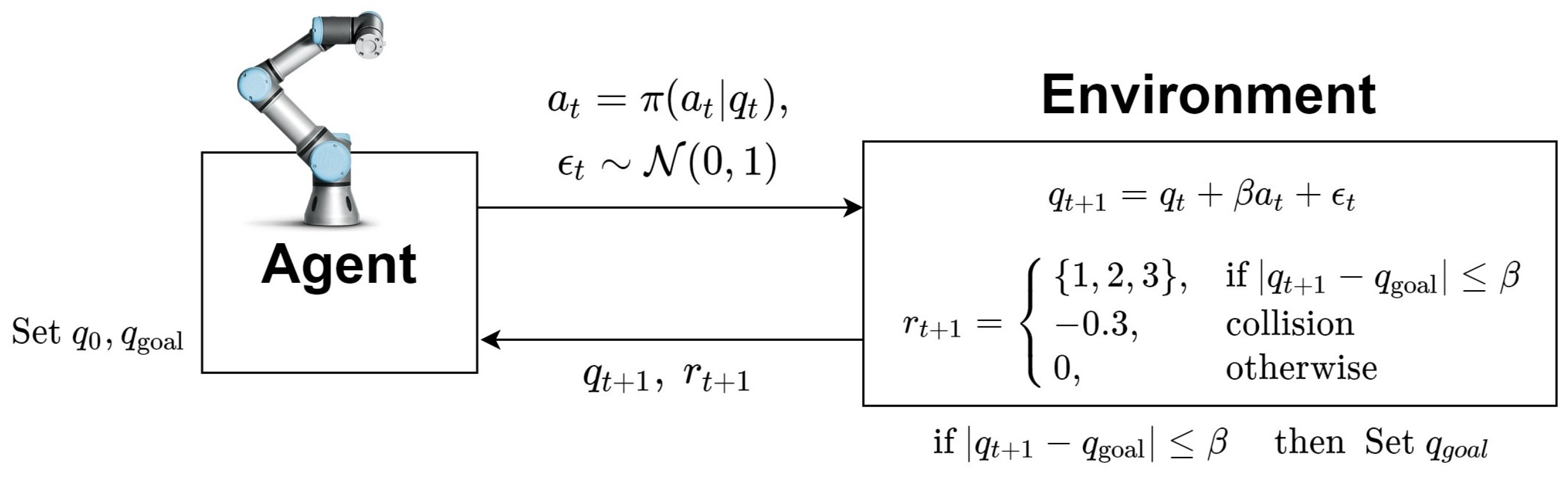
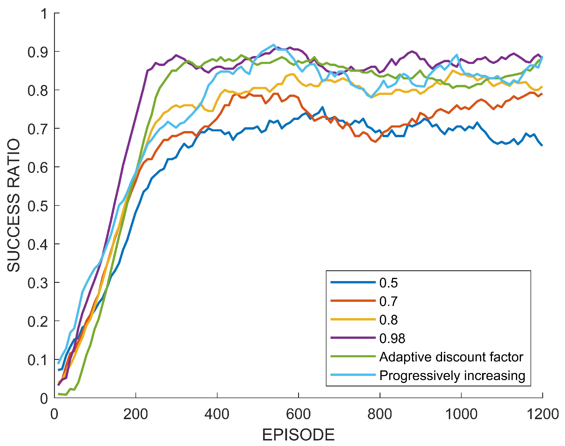
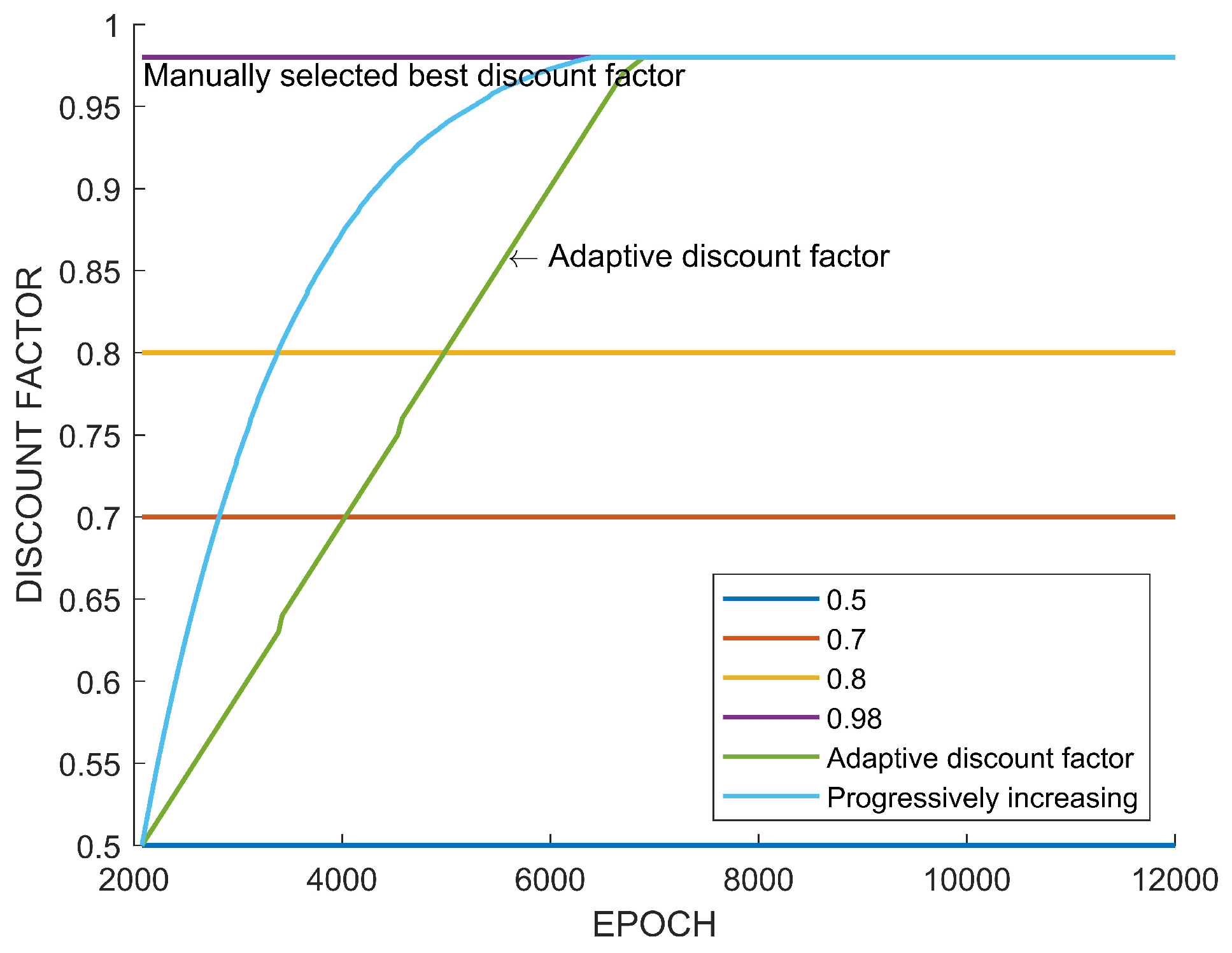
5.2. Motion Planning
5.3. Analysis and Discussion
6. Conclusions
Author Contributions
Funding
Institutional Review Board Statement
Informed Consent Statement
Data Availability Statement
Conflicts of Interest
Appendix A
| Algorithm A1: Adaptive Discount Factor in PPO |
|
| Algorithm A2: Adaptive Discount Factor in SAC |
|
References
- Sutton, R.S.; Barto, A.G. Reinforcement Learning: An Introduction; MIT Press: Cambridge, MA, USA, 2018. [Google Scholar]
- Mnih, V.; Kavukcuoglu, K.; Silver, D.; Rusu, A.A.; Veness, J.; Bellemare, M.G.; Graves, A.; Riedmiller, M.; Fidjeland, A.K.; Ostrovski, G.; et al. Human-level control through deep reinforcement learning. Nature 2015, 518, 529–533. [Google Scholar] [CrossRef] [PubMed]
- Berseth, G.; Geng, D.; Devin, C.M.; Rhinehart, N.; Finn, C.; Jayaraman, D.; Levine, S. SMiRL: Surprise Minimizing Reinforcement Learning in Unstable Environments. In Proceedings of the International Conference on Learning Representations, Addis Ababa, Ethiopia, 26–30 April 2020. [Google Scholar]
- Garcıa, J.; Fernández, F. A comprehensive survey on safe reinforcement learning. J. Mach. Learn. Res. 2015, 16, 1437–1480. [Google Scholar]
- Van Hasselt, H.; Guez, A.; Silver, D. Deep reinforcement learning with double q-learning. In Proceedings of the AAAI Conference on Artificial Intelligence, Phoenix, AZ, USA, 12–17 February 2016; Volume 30. [Google Scholar]
- Fujimoto, S.; Hoof, H.; Meger, D. Addressing function approximation error in actor-critic methods. In Proceedings of the International Conference on Machine Learning, PMLR, Stockholm, Sweden, 10–15 July 2018; pp. 1587–1596. [Google Scholar]
- Hessel, M.; Modayil, J.; Van Hasselt, H.; Schaul, T.; Ostrovski, G.; Dabney, W.; Horgan, D.; Piot, B.; Azar, M.; Silver, D. Rainbow: Combining improvements in deep reinforcement learning. In Proceedings of the Thirty-Second AAAI Conference on Artificial Intelligence, New Orleans, LA, USA, 2–7 February 2018. [Google Scholar]
- Thrun, S.; Schwartz, A. Issues in using function approximation for reinforcement learning. In Proceedings of the 1993 Connectionist Models Summer School; Lawrence Erlbaum: Hillsdale, NJ, USA, 1993; Volume 6, pp. 1–9. [Google Scholar]
- Badia, A.P.; Sprechmann, P.; Vitvitskyi, A.; Guo, D.; Piot, B.; Kapturowski, S.; Tieleman, O.; Arjovsky, M.; Pritzel, A.; Bolt, A.; et al. Never Give Up: Learning Directed Exploration Strategies. In Proceedings of the International Conference on Learning Representations, New Orleans, LA, USA, 6–9 May 2019. [Google Scholar]
- Badia, A.P.; Piot, B.; Kapturowski, S.; Sprechmann, P.; Vitvitskyi, A.; Guo, Z.D.; Blundell, C. Agent57: Outperforming the atari human benchmark. In Proceedings of the International Conference on Machine Learning, PMLR, Virtual, 13–18 July 2020; pp. 507–517. [Google Scholar]
- Amit, R.; Meir, R.; Ciosek, K. Discount factor as a regularizer in reinforcement learning. In Proceedings of the International Conference on Machine Learning, PMLR, Virtual, 13–18 July 2020; pp. 269–278. [Google Scholar]
- Van Seijen, H.; Fatemi, M.; Tavakoli, A. Using a logarithmic mapping to enable lower discount factors in reinforcement learning. Adv. Neural Inf. Process. Syst. 2019, 33, 14134–14144. [Google Scholar]
- Schulman, J.; Wolski, F.; Dhariwal, P.; Radford, A.; Klimov, O. Proximal policy optimization algorithms. arXiv 2017, arXiv:1707.06347. [Google Scholar]
- Mnih, V.; Badia, A.P.; Mirza, M.; Graves, A.; Lillicrap, T.; Harley, T.; Silver, D.; Kavukcuoglu, K. Asynchronous methods for deep reinforcement learning. In Proceedings of the International Conference on Machine Learning, New York, NY, USA, 20–22 June 2016; pp. 1928–1937. [Google Scholar]
- François-Lavet, V.; Fonteneau, R.; Ernst, D. How to Discount Deep Reinforcement Learning: Towards New Dynamic Strategies. In Proceedings of the NIPS 2015 Workshop on Deep Reinforcement Learning, Montréal, QC, Canada, 11 December 2015. [Google Scholar]
- Haarnoja, T.; Zhou, A.; Abbeel, P.; Levine, S. Soft actor-critic: Off-policy maximum entropy deep reinforcement learning with a stochastic actor. In Proceedings of the International Conference on Machine Learning, Stockholm, Sweden, 10–15 July 2018; pp. 1861–1870. [Google Scholar]
- Chen, X.; Wang, C.; Zhou, Z.; Ross, K.W. Randomized Ensembled Double Q-Learning: Learning Fast Without a Model. In Proceedings of the International Conference on Learning Representations, Addis Ababa, Ethiopia, 26–30 April 2020. [Google Scholar]
- Dabney, W.; Ostrovski, G.; Silver, D.; Munos, R. Implicit quantile networks for distributional reinforcement learning. In Proceedings of the International Conference on Machine Learning, Stockholm, Sweden, 10–15 July 2018; pp. 1096–1105. [Google Scholar]
- Mavrin, B.; Yao, H.; Kong, L.; Wu, K.; Yu, Y. Distributional reinforcement learning for efficient exploration. In Proceedings of the International Conference on Machine Learning, Long Beach, CA, USA, 9–15 June 2019; pp. 4424–4434. [Google Scholar]
- Yang, D.; Zhao, L.; Lin, Z.; Qin, T.; Bian, J.; Liu, T.Y. Fully parameterized quantile function for distributional reinforcement learning. Adv. Neural Inf. Process. Syst. 2019, 33, 6193–6202. [Google Scholar]
- Kapturowski, S.; Ostrovski, G.; Quan, J.; Munos, R.; Dabney, W. Recurrent experience replay in distributed reinforcement learning. In Proceedings of the International Conference on Learning Representations, Vancouver, BC, Canada, 30 April–3 May 2018. [Google Scholar]
- Fedus, W.; Gelada, C.; Bengio, Y.; Bellemare, M.G.; Larochelle, H. Hyperbolic discounting and learning over multiple horizons. arXiv 2019, arXiv:1902.06865. [Google Scholar]
- Sutton, R.S.; McAllester, D.; Singh, S.; Mansour, Y. Policy gradient methods for reinforcement learning with function approximation. Adv. Neural Inf. Process. Syst. 1999, 12, 1057–1063. [Google Scholar]
- Naik, A.; Shariff, R.; Yasui, N.; Yao, H.; Sutton, R.S. Discounted reinforcement learning is not an optimization problem. arXiv 2019, arXiv:1910.02140. [Google Scholar]
- Schulman, J.; Levine, S.; Abbeel, P.; Jordan, M.; Moritz, P. Trust region policy optimization. In Proceedings of the International Conference on Machine Learning, Lille, France, 7–9 July 2015; pp. 1889–1897. [Google Scholar]
- Haarnoja, T.; Tang, H.; Abbeel, P.; Levine, S. Reinforcement learning with deep energy-based policies. In Proceedings of the International Conference on Machine Learning, Sydney, Australia, 6–11 August 2017; pp. 1352–1361. [Google Scholar]
- Algorta, S.; Şimşek, Ö. The game of tetris in machine learning. arXiv 2019, arXiv:1905.01652. [Google Scholar]
- Demaine, E.D.; Hohenberger, S.; Liben-Nowell, D. Tetris is hard, even to approximate. In Proceedings of the International Computing and Combinatorics Conference, Big Sky, MT, USA, 25–28 July 2003; Springer: New York, NY, USA, 2003; pp. 351–363. [Google Scholar]
- Gabillon, V.; Ghavamzadeh, M.; Scherrer, B. Approximate dynamic programming finally performs well in the game of Tetris. Adv. Neural Inf. Process. Syst. 2013, 26, 1754–1762. [Google Scholar]
- Vinyals, O.; Babuschkin, I.; Czarnecki, W.M.; Mathieu, M.; Dudzik, A.; Chung, J.; Choi, D.H.; Powell, R.; Ewalds, T.; Georgiev, P.; et al. Grandmaster level in StarCraft II using multi-agent reinforcement learning. Nature 2019, 575, 350–354. [Google Scholar] [CrossRef] [PubMed]
- Gu, S.; Holly, E.; Lillicrap, T.; Levine, S. Deep reinforcement learning for robotic manipulation with asynchronous off-policy updates. In Proceedings of the 2017 IEEE International Conference on Robotics and Automation (ICRA), Singapore, 29 May–3 June 2017; IEEE: Providence, RI, USA, 2017; pp. 3389–3396. [Google Scholar]
- Kalashnikov, D.; Irpan, A.; Pastor, P.; Ibarz, J.; Herzog, A.; Jang, E.; Quillen, D.; Holly, E.; Kalakrishnan, M.; Vanhoucke, V.; et al. Scalable deep reinforcement learning for vision-based robotic manipulation. In Proceedings of the Conference on Robot Learning, Zurich, Switzerland, 29–31 October 2018; pp. 651–673. [Google Scholar]
- Spong, M.W.; Hutchinson, S.; Vidyasagar, M. Robot Modeling and Control; Wiley: New York, NY, USA, 2006; Volume 3. [Google Scholar]
- Frank, M.; Leitner, J.; Stollenga, M.; Förster, A.; Schmidhuber, J. Curiosity driven reinforcement learning for motion planning on humanoids. Front. Neurorobot. 2014, 7, 25. [Google Scholar] [CrossRef] [PubMed]
- Prianto, E.; Kim, M.; Park, J.H.; Bae, J.H.; Kim, J.S. Path planning for multi-arm manipulators using deep reinforcement learning: Soft actor–critic with hindsight experience replay. Sensors 2020, 20, 5911. [Google Scholar] [CrossRef] [PubMed]
- Zhu, H.; Yu, J.; Gupta, A.; Shah, D.; Hartikainen, K.; Singh, A.; Kumar, V.; Levine, S. The Ingredients of Real World Robotic Reinforcement Learning. In Proceedings of the International Conference on Learning Representations, New Orleans, LA, USA, 6–9 May 2019. [Google Scholar]


| 0 | 1 | 2 | 3 | 4 | ||
| r | 0 | 1 | 3 | 6 | 10 |
| Maximum Score | Average Score | ||
|---|---|---|---|
| Adaptive discount factor | 318 | 139.28 | 0.7214 |
| Increasing discount factor | 37 | 29.94 | 0.99 |
| Fixed discount factor 1 | 49 | 25.98 | 0.99 |
| Fixed discount factor 2 | 115 | 65.03 | 0.9 |
| Fixed discount factor 3 | 179 | 97.94 | 0.7 |
| Fixed discount factor 4 | 61 | 35.87 | 0.5 |
| Success Rate | ||
|---|---|---|
| Adaptive discount factor | 0.8846 | 0.98 |
| Increasing discount factor | 0.8915 | 0.98 |
| Fixed discount factor 1 | 0.8884 | 0.98 |
| Fixed discount factor 2 | 0.8222 | 0.8 |
| Fixed discount factor 3 | 0.7833 | 0.7 |
| Fixed discount factor 4 | 0.6588 | 0.5 |
| Maximum | Averages | ||
|---|---|---|---|
| Adaptive discount factor | 464 | 287.77 | 0.7591 |
| Increasing discount factor | 409 | 194.74 | 0.99 |
| Fixed discount factor 1 | 256 | 155.76 | 0.99 |
| Fixed discount factor 2 | 351 | 212.87 | 0.90 |
| Fixed discount factor 3 | 421 | 231.86 | 0.75 |
| Fixed discount factor 4 | 388 | 189.09 | 0.5 |
Publisher’s Note: MDPI stays neutral with regard to jurisdictional claims in published maps and institutional affiliations. |
© 2022 by the authors. Licensee MDPI, Basel, Switzerland. This article is an open access article distributed under the terms and conditions of the Creative Commons Attribution (CC BY) license (https://creativecommons.org/licenses/by/4.0/).
Share and Cite
Kim, M.; Kim, J.-S.; Choi, M.-S.; Park, J.-H. Adaptive Discount Factor for Deep Reinforcement Learning in Continuing Tasks with Uncertainty. Sensors 2022, 22, 7266. https://doi.org/10.3390/s22197266
Kim M, Kim J-S, Choi M-S, Park J-H. Adaptive Discount Factor for Deep Reinforcement Learning in Continuing Tasks with Uncertainty. Sensors. 2022; 22(19):7266. https://doi.org/10.3390/s22197266
Chicago/Turabian StyleKim, MyeongSeop, Jung-Su Kim, Myoung-Su Choi, and Jae-Han Park. 2022. "Adaptive Discount Factor for Deep Reinforcement Learning in Continuing Tasks with Uncertainty" Sensors 22, no. 19: 7266. https://doi.org/10.3390/s22197266
APA StyleKim, M., Kim, J.-S., Choi, M.-S., & Park, J.-H. (2022). Adaptive Discount Factor for Deep Reinforcement Learning in Continuing Tasks with Uncertainty. Sensors, 22(19), 7266. https://doi.org/10.3390/s22197266