


Bearing Fault Diagnosis Based on Randomized Fisher Discriminant Analysis


Abstract
1. Introduction
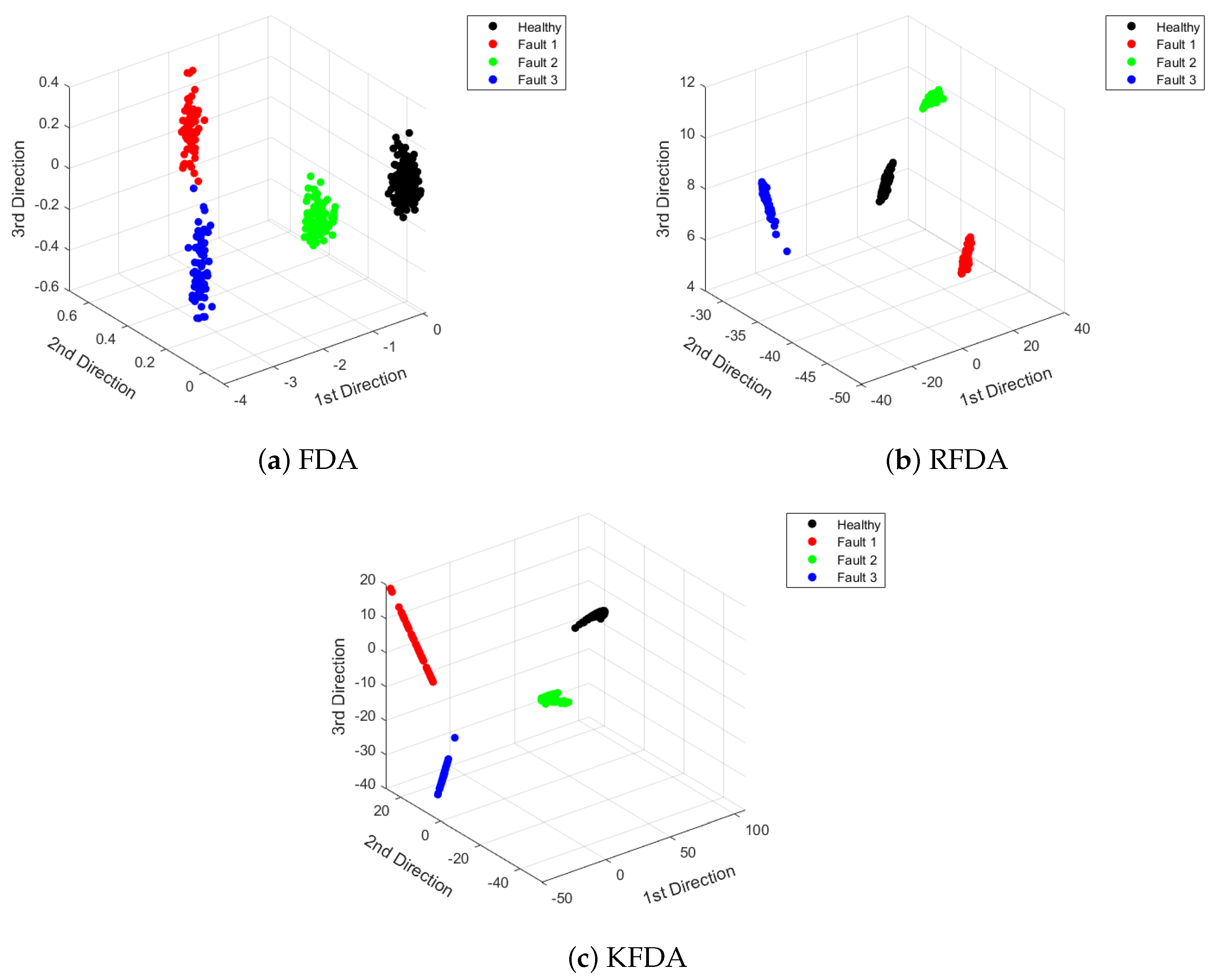
- RFDA, a nonlinear variant of FDA, is utilized for bearing fault diagnosis. The RFDA-based method can achieve similar performance to the KFDA-based method, while the computational burden is remarkably reduced.
- Two widely used bearing datasets are employed to validate the effectiveness of the proposed RFDA-based bearing fault diagnosis method. Results show the superior performance of the proposed method over other related methods.
2. Related Works
2.1. Fisher Discriminant Analysis
2.2. Random Fourier Feature Map
3. RFDA-Based Fault Diagnosis
3.1. Time-Domain Feature Extraction
3.2. RFDA Model Training
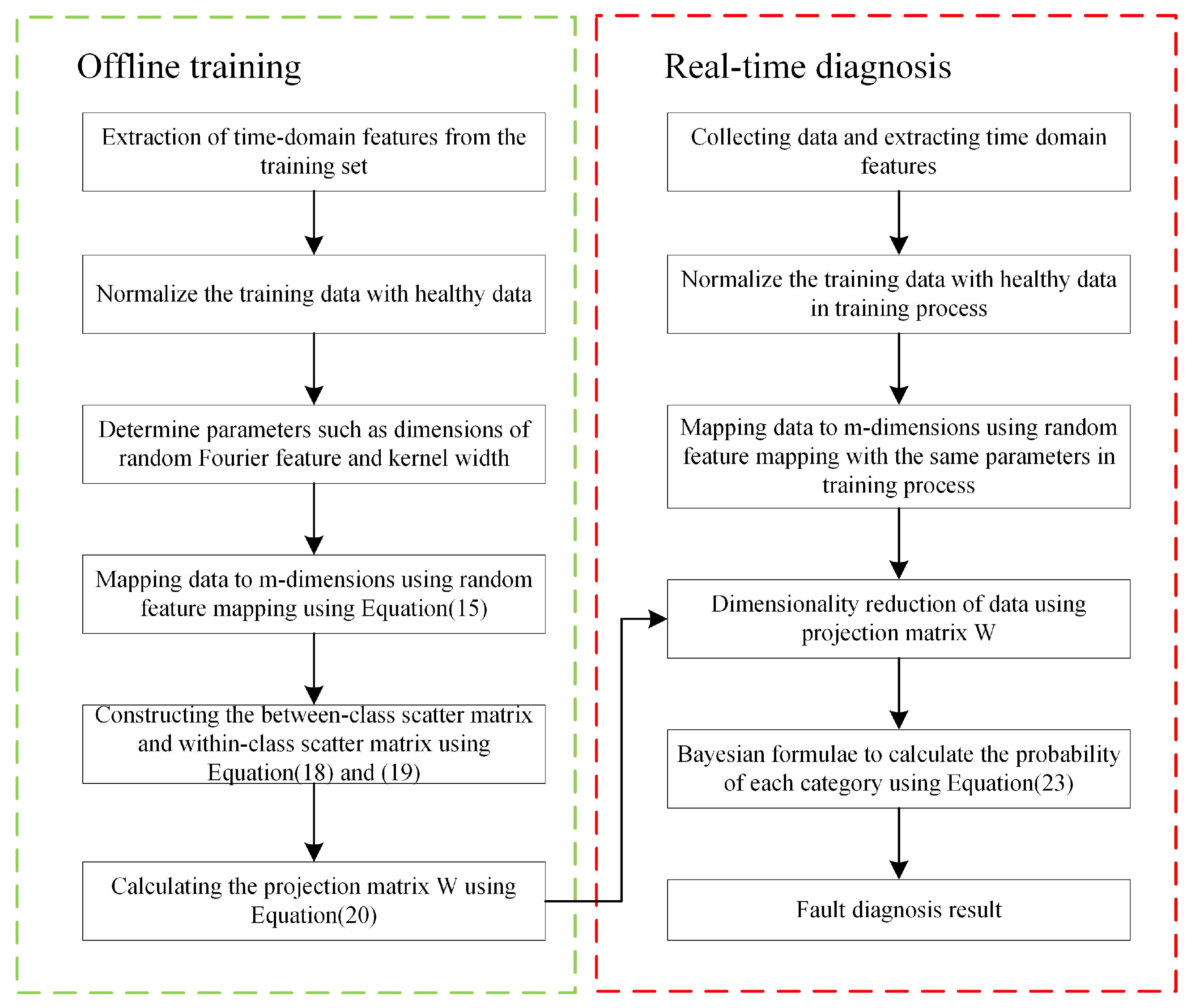
3.3. RFDA-Based Bearing Fault Diagnosis Scheme
4. Experiments and Results
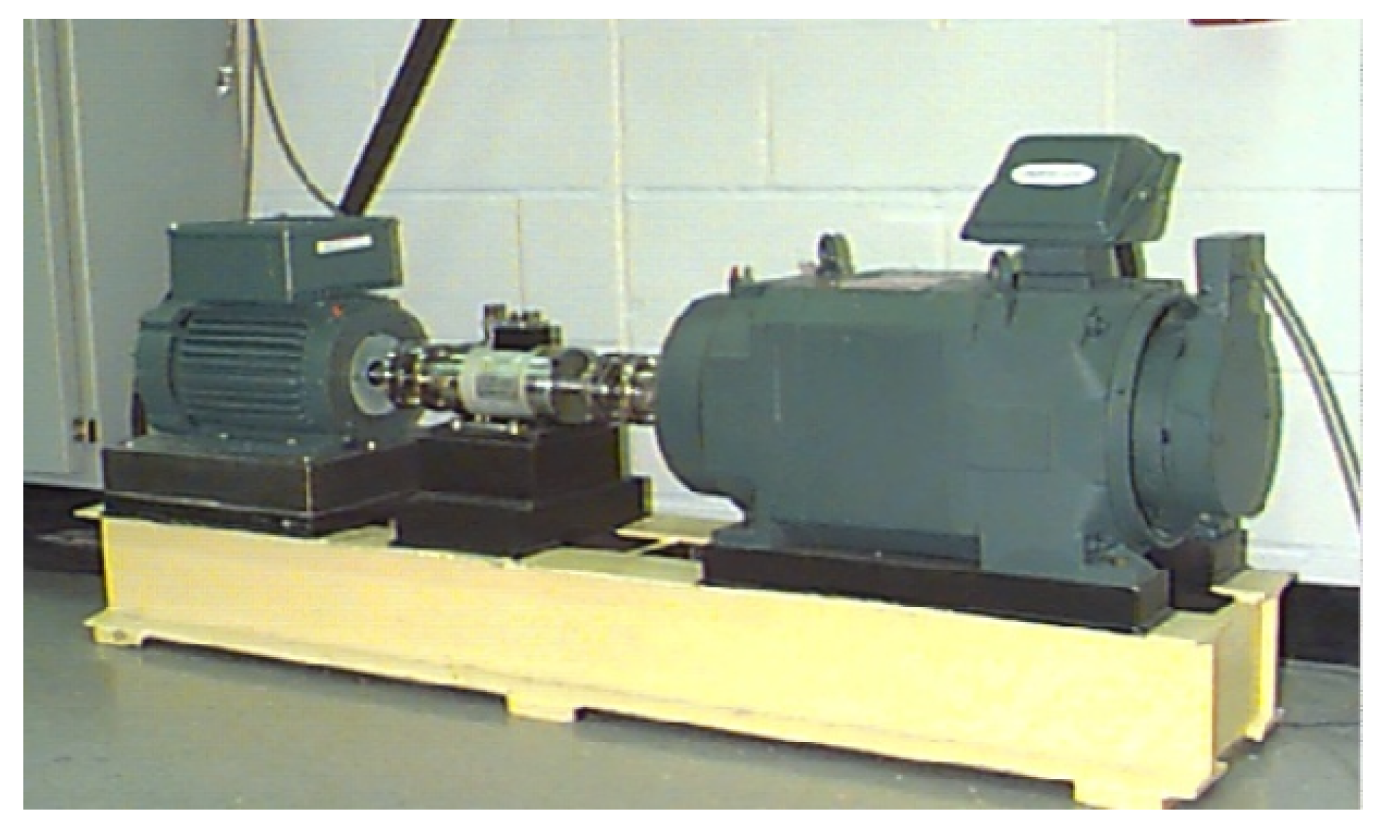
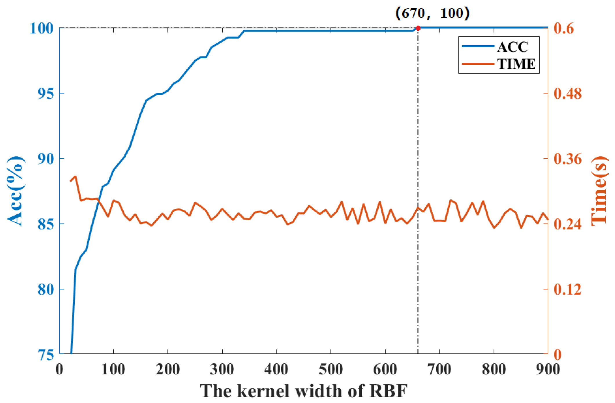
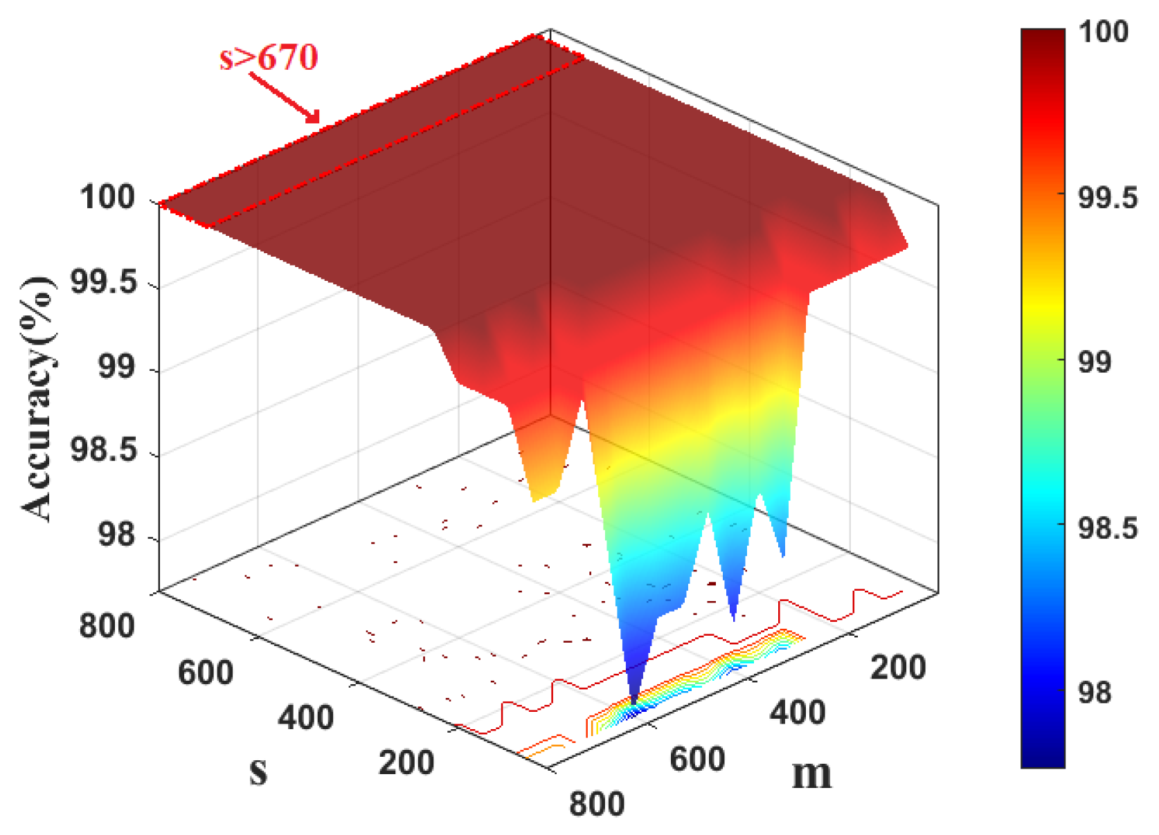
4.1. Case 1: CWRU Dataset
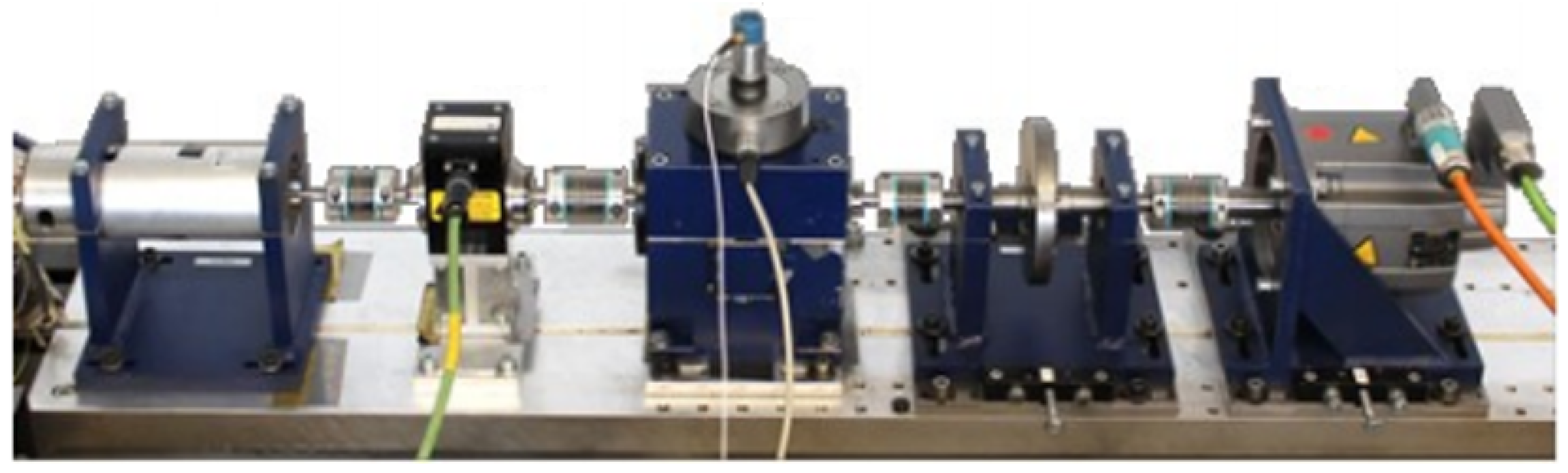
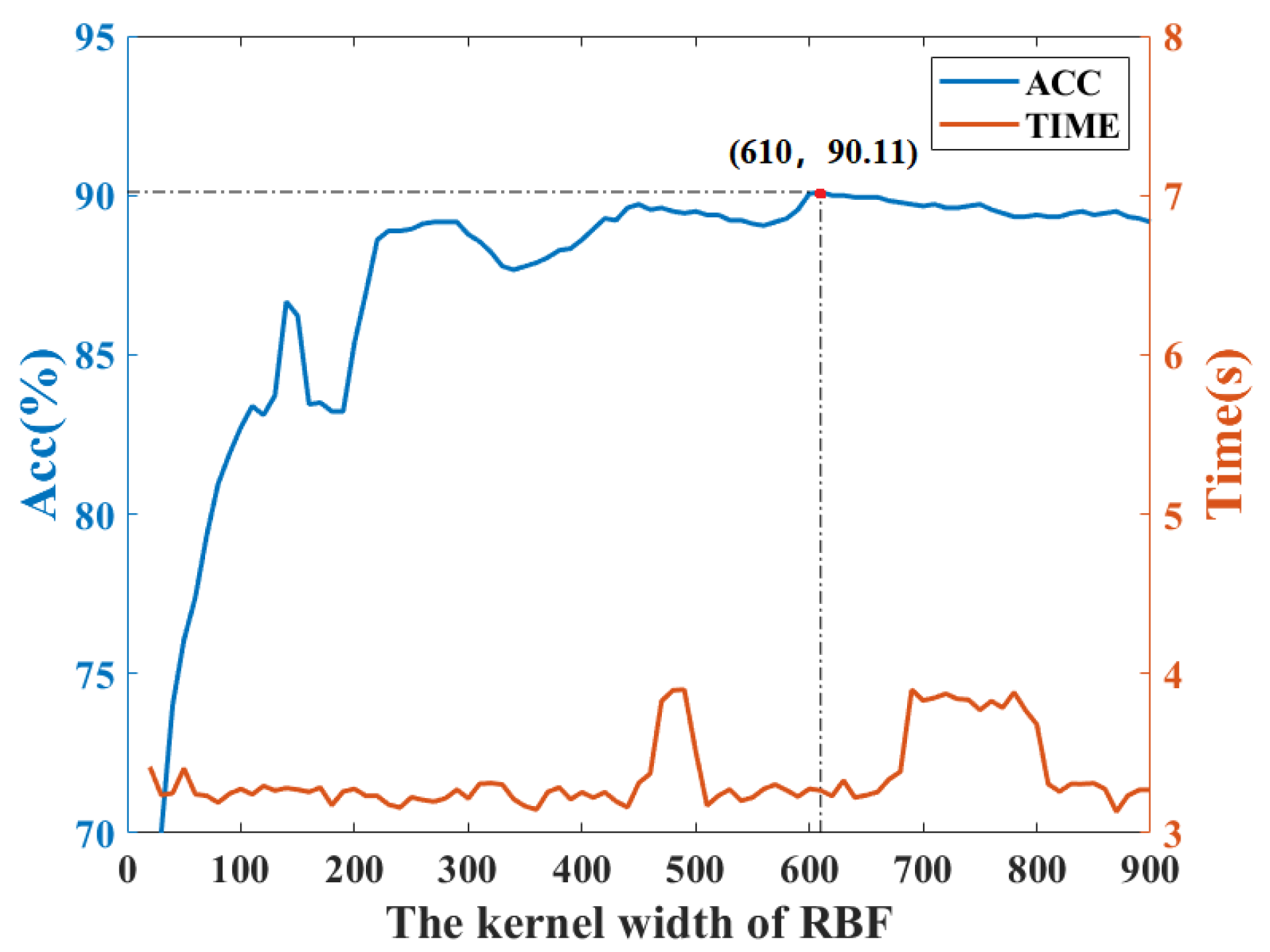
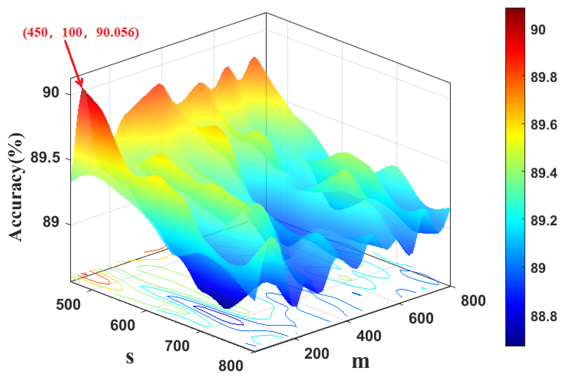
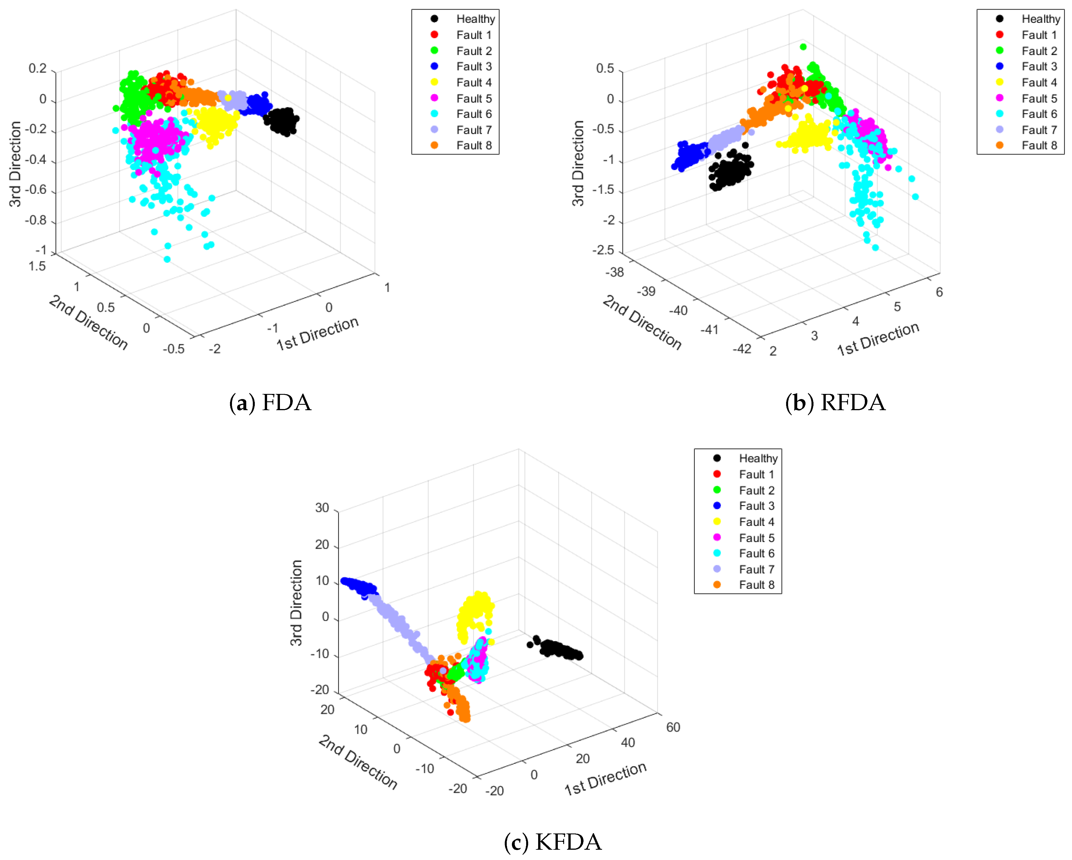
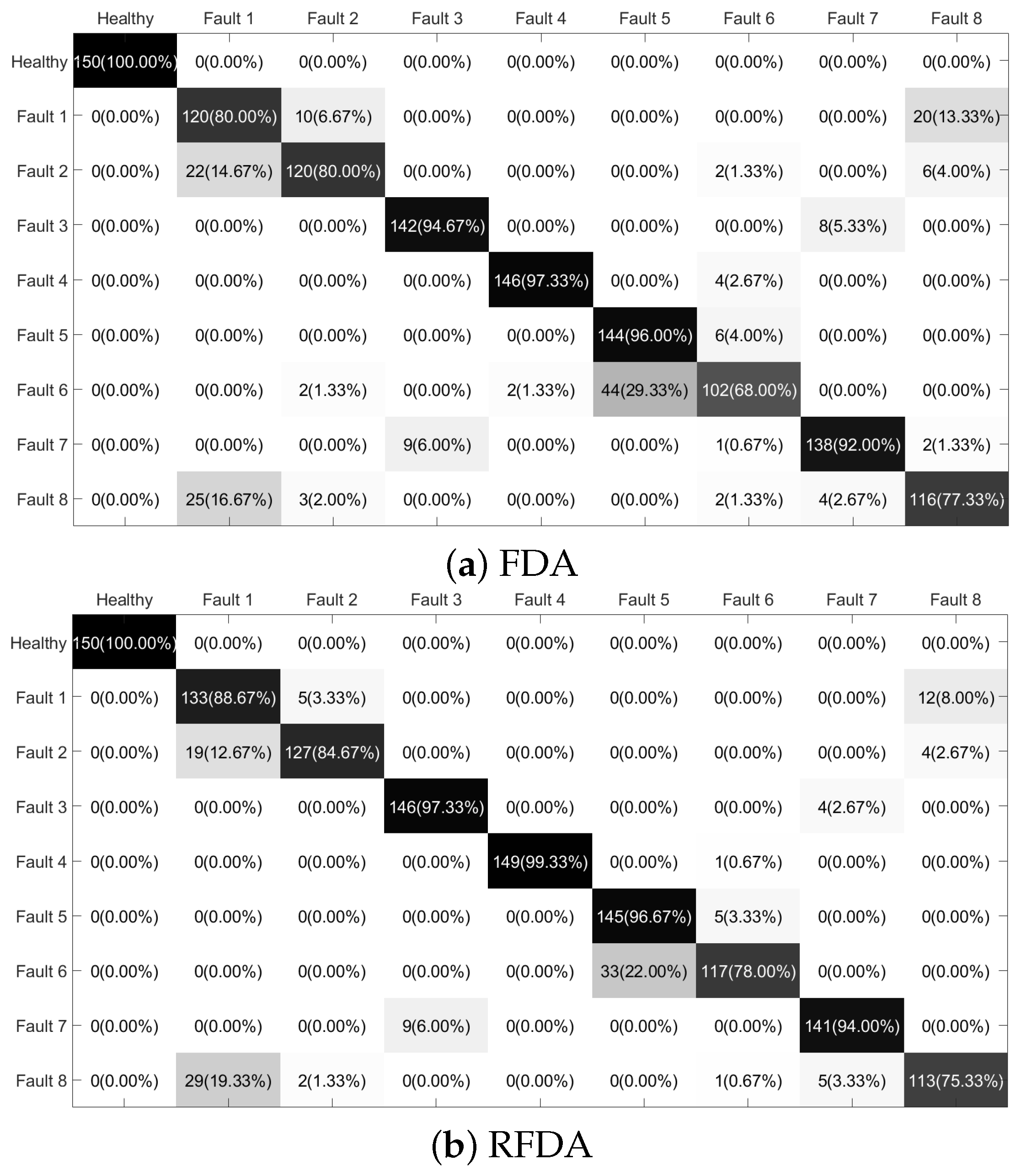
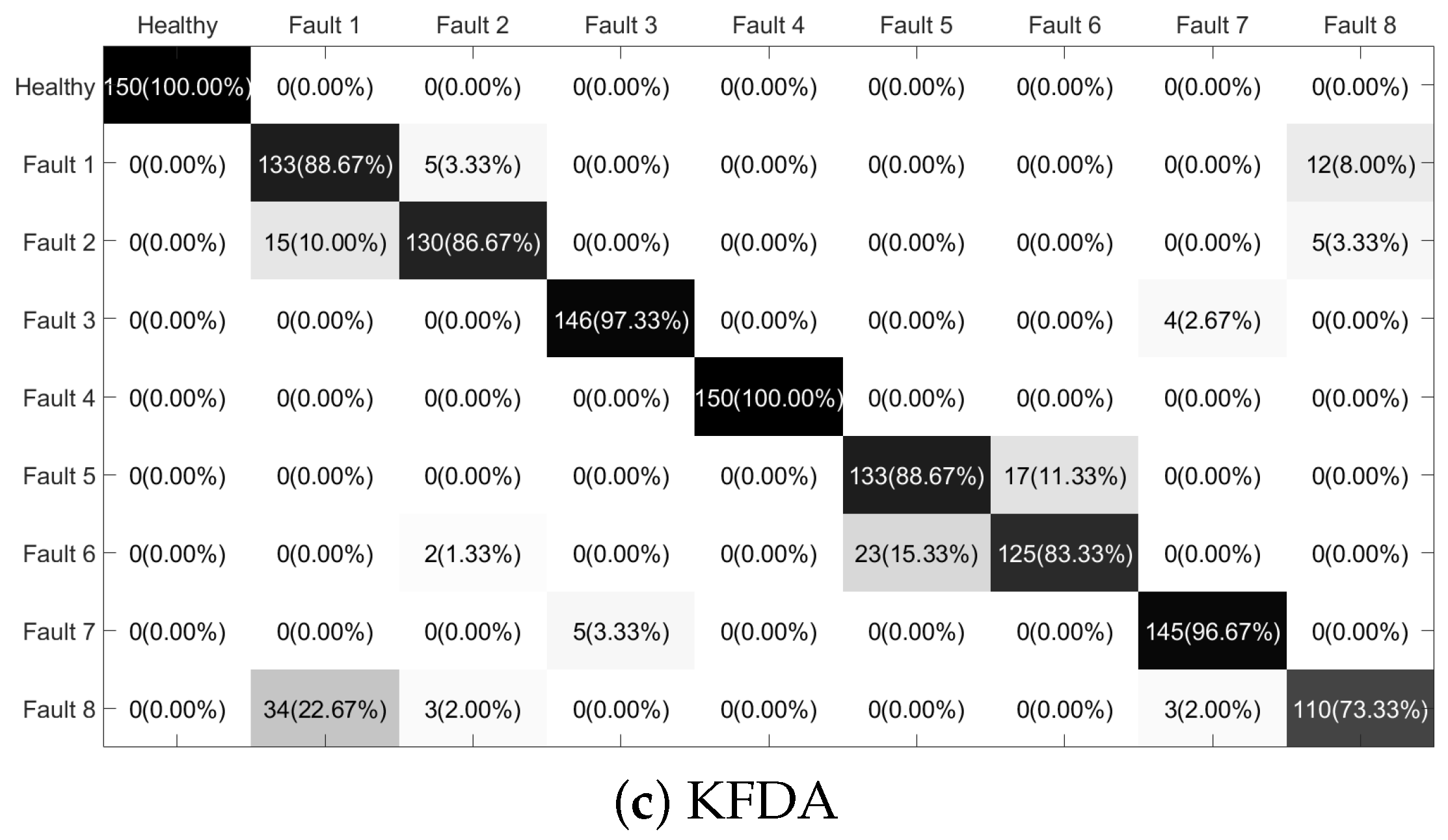
4.2. Case 2: PU Dataset
5. Conclusions
Author Contributions
Funding
Institutional Review Board Statement
Informed Consent Statement
Data Availability Statement
Acknowledgments
Conflicts of Interest
References
- Hoang, D.T.; Kang, H.J. A survey on deep learning based bearing fault diagnosis. Neurocomputing 2019, 335, 327–335. [Google Scholar] [CrossRef]
- Zhang, S.; Zhang, S.; Wang, B.; Habetler, T.G. Deep learning algorithms for bearing fault diagnostics—A comprehensive review. IEEE Access 2020, 8, 29857–29881. [Google Scholar] [CrossRef]
- Zhang, Y.; Gao, Q.; Lu, Y.; Sun, D.; Xia, Y.; Peng, X. A novel intelligent method for bearing fault diagnosis based on Hermitian scale-energy spectrum. IEEE Sens. J. 2018, 18, 6743–6755. [Google Scholar] [CrossRef]
- Liu, L.; Chen, L.; Wang, Z.; Liu, D. Early fault detection of planetary gearbox based on acoustic emission and improved variational mode decomposition. IEEE Sens. J. 2020, 21, 1735–1745. [Google Scholar] [CrossRef]
- Li, X.; Yang, Y.; Pan, H.; Cheng, J.; Cheng, J. A novel deep stacking least squares support vector machine for rolling bearing fault diagnosis. Comput. Ind. 2019, 110, 36–47. [Google Scholar] [CrossRef]
- Naha, A.; Samanta, A.K.; Routray, A.; Deb, A.K. Low complexity motor current signature analysis using sub-Nyquist strategy with reduced data length. IEEE Trans. Instrum. Meas. 2017, 66, 3249–3259. [Google Scholar] [CrossRef]
- Nikula, R.P.; Karioja, K.; Pylvänäinen, M.; Leiviskä, K. Automation of low-speed bearing fault diagnosis based on autocorrelation of time domain features. Mech. Syst. Sig. Process. 2020, 138, 106572. [Google Scholar] [CrossRef]
- Nayana, B.; Geethanjali, P. Analysis of statistical time-domain features effectiveness in identification of bearing faults from vibration signal. IEEE Sens. J. 2017, 17, 5618–5625. [Google Scholar] [CrossRef]
- Lu, Y.; Wang, Z.; Zhu, D.; Gao, Q.; Sun, D. Bearing fault diagnosis based on clustering and sparse representation in frequency domain. IEEE Trans. Instrum. Meas. 2021, 70, 1–14. [Google Scholar] [CrossRef]
- Zhang, Y.; Xing, K.; Bai, R.; Sun, D.; Meng, Z. An enhanced convolutional neural network for bearing fault diagnosis based on time–frequency image. Measurement 2020, 157, 107667. [Google Scholar] [CrossRef]
- De Moura, E.; Souto, C.; Silva, A.; Irmao, M. Evaluation of principal component analysis and neural network performance for bearing fault diagnosis from vibration signal processed by RS and DF analyses. Mech. Syst. Sig. Process. 2011, 25, 1765–1772. [Google Scholar] [CrossRef]
- Yu, J. Local and nonlocal preserving projection for bearing defect classification and performance assessment. IEEE Trans. Ind. Electron. 2011, 59, 2363–2376. [Google Scholar] [CrossRef]
- Ambrożkiewicz, B.; Syta, A.; Gassner, A.; Georgiadis, A.; Litak, G.; Meier, N. The influence of the radial internal clearance on the dynamic response of self-aligning ball bearings. Mech. Syst. Sig. Process. 2022, 171, 108954. [Google Scholar] [CrossRef]
- Syta, A.; Czarnigowski, J.; Jakliński, P. Detection of cylinder misfire in an aircraft engine using linear and non-linear signal analysis. Measurement 2021, 174, 108982. [Google Scholar] [CrossRef]
- Tu, D.; Zheng, J.; Jiang, Z.; Pan, H. Multiscale distribution entropy and t-distributed stochastic neighbor embedding-based fault diagnosis of rolling bearings. Entropy 2018, 20, 360. [Google Scholar] [CrossRef]
- Joswiak, M.; Peng, Y.; Castillo, I.; Chiang, L.H. Dimensionality reduction for visualizing industrial chemical process data. Control Eng. Pract. 2019, 93, 104189. [Google Scholar] [CrossRef]
- Mao, W.; Feng, W.; Liu, Y.; Zhang, D.; Liang, X. A new deep auto-encoder method with fusing discriminant information for bearing fault diagnosis. Mech. Syst. Sig. Process. 2021, 150, 107233. [Google Scholar] [CrossRef]
- Zhang, S.; Ye, F.; Wang, B.; Habetler, T.G. Semi-Supervised Bearing Fault Diagnosis and Classification Using Variational Autoencoder-Based Deep Generative Models. IEEE Sens. J. 2021, 21, 6476–6486. [Google Scholar] [CrossRef]
- Jin, X.; Zhao, M.; Chow, T.W.; Pecht, M. Motor bearing fault diagnosis using trace ratio linear discriminant analysis. IEEE Trans. Ind. Electron. 2013, 61, 2441–2451. [Google Scholar] [CrossRef]
- Zhou, Y.; Yan, S.; Ren, Y.; Liu, S. Rolling bearing fault diagnosis using transient-extracting transform and linear discriminant analysis. Measurement 2021, 178, 109298. [Google Scholar] [CrossRef]
- Mika, S.; Ratsch, G.; Weston, J.; Scholkopf, B.; Mullers, K.R. Fisher discriminant analysis with kernels. In Proceedings of the Neural Networks for Signal Processing IX: Proceedings of the 1999 IEEE Signal Processing Society Workshop (Cat. No. 98th8468), Madison, WI, USA, 25 August 1999; IEEE: Piscataway, NJ, USA, 1999; pp. 41–48. [Google Scholar]
- Van, M.; Kang, H.J. Bearing defect classification based on individual wavelet local fisher discriminant analysis with particle swarm optimization. IEEE Trans. Ind. Inf. 2015, 12, 124–135. [Google Scholar] [CrossRef]
- Jiang, L.; Xuan, J.; Shi, T. Feature extraction based on semi-supervised kernel Marginal Fisher analysis and its application in bearing fault diagnosis. Mech. Syst. Sig. Process. 2013, 41, 113–126. [Google Scholar] [CrossRef]
- Tao, X.; Ren, C.; Li, Q.; Guo, W.; Liu, R.; He, Q.; Zou, J. Bearing defect diagnosis based on semi-supervised kernel Local Fisher Discriminant Analysis using pseudo labels. ISA Trans. 2021, 110, 394–412. [Google Scholar] [CrossRef]
- Li, J.; Cui, P. Improved kernel fisher discriminant analysis for fault diagnosis. Expert Syst. Appl. 2009, 36, 1423–1432. [Google Scholar] [CrossRef]
- Liu, Z.; Qu, J.; Zuo, M.J.; Xu, H.b. Fault level diagnosis for planetary gearboxes using hybrid kernel feature selection and kernel Fisher discriminant analysis. Int. J. Adv. Manuf. Technol. 2013, 67, 1217–1230. [Google Scholar] [CrossRef]
- Rahimi, A.; Recht, B. Random features for large-scale kernel machines. In Advances in Neural Information Processing Systems 20 (NIPS 2007); Citeseer: Princeton, NJ, USA, 2007; Volume 20, pp. 1177–1184. [Google Scholar]
- Lopez-Paz, D.; Sra, S.; Smola, A.; Ghahramani, Z.; Schölkopf, B. Randomized nonlinear component analysis. In Proceedings of the International Conference on Machine Learning, PMLR, Bejing, China, 22–24 June 2014; pp. 1359–1367. [Google Scholar]
- Jayaprakash, C.; Damodaran, B.B.; Viswanathan, S.; Soman, K.P. Randomized independent component analysis and linear discriminant analysis dimensionality reduction methods for hyperspectral image classification. J. Appl. Remote Sens. 2020, 14, 036507. [Google Scholar] [CrossRef]
- Ye, H.; Li, Y.; Chen, C.; Zhang, Z. Fast Fisher discriminant analysis with randomized algorithms. Pattern Recognit. 2017, 72, 82–92. [Google Scholar] [CrossRef]
- Fukunaga, K. Introduction to Statistical Pattern Recognition; Elsevier: Amsterdam, The Netherlands, 2013. [Google Scholar]
- Funktionen, M. Stieltjessche Integrale und harmonische Analyse. Math. Ann. 1933, 108, 378–410. [Google Scholar]
- Sutherland, D.J.; Schneider, J. On the error of random Fourier features. arXiv 2015, arXiv:1506.02785. [Google Scholar]
- Chiang, L.H.; Russell, E.L.; Braatz, R.D. Fault diagnosis in chemical processes using Fisher discriminant analysis, discriminant partial least squares, and principal component analysis. Chemom. Intell. Lab. Syst. 2000, 50, 243–252. [Google Scholar] [CrossRef]
- Ge, Z.; Zhong, S.; Zhang, Y. Semisupervised Kernel Learning for FDA Model and its Application for Fault Classification in Industrial Processes. IEEE Trans. Ind. Inf. 2016, 12, 1403–1411. [Google Scholar] [CrossRef]
- Zhang, J.F.; Huang, Z.C. Kernel Fisher discriminant analysis for bearing fault diagnosis. In Proceedings of the 2005 International Conference on Machine Learning and Cybernetics, Guangzhou, China, 18–21 August 2005; IEEE: Piscataway, NJ, USA, 2005; Volume 5, pp. 3216–3220. [Google Scholar]
- Lessmeier, C.; Kimotho, J.K.; Zimmer, D.; Sextro, W. Condition monitoring of bearing damage in electromechanical drive systems by using motor current signals of electric motors: A benchmark data set for data-driven classification. In Proceedings of the European Conference of the Prognostics and Health Management Society, Bilbao, Spain, 5–8 July 2016; Citeseer: Princeton, NJ, USA, 2016; pp. 5–8. [Google Scholar]


| Features | Equations |
|---|---|
| Peak | |
| Peak-to-peak | |
| Mean | |
| Absolute mean amplitude | |
| Square root amplitude | |
| Variance | |
| Standard deviation | |
| Root mean square | |
| Kurtosis | |
| Skewness | |
| Peak factor | |
| Impulsive factor |
| Bearing State | Fault Location | Train Number | Test Number | Characteristic Frequency (Hz) |
|---|---|---|---|---|
| Health | / | 50 | 188 | 29.95 |
| Fault 1 | inner ring | 50 | 68 | 162.1852 |
| Fault 2 | rolling element | 50 | 69 | 141.0907667 |
| Fault 3 | outer ring | 50 | 69 | 107.305 |
| Method | Mean Acc | Mean Time (s) |
|---|---|---|
| FDA | 100% | 0.1146 |
| KFDA | 100% | 0.2647 |
| RFDA | 100% | 0.1232 |
| Bearing State | Bearing Code | Train Number | Test Number |
|---|---|---|---|
| Health | K004 | 100 | 150 |
| Fault 1 | KA04 | 100 | 150 |
| Fault 2 | KA16 | 100 | 150 |
| Fault 3 | KA22 | 100 | 150 |
| Fault 4 | KA30 | 100 | 150 |
| Fault 5 | KB23 | 100 | 150 |
| Fault 6 | KB24 | 100 | 150 |
| Fault 7 | KB27 | 100 | 150 |
| Fault 8 | KI16 | 100 | 150 |
| Bearing State | Bearing Code | Fault Position | Description |
|---|---|---|---|
| Health | K004 | Healthy | Run-in period 5 h |
| Fault 1 | KA04 | Outer ring (SP, S, Level 1) | Caused by fatigue and pitting |
| Fault 2 | KA16 | Outer ring (SP, R, Level 2) | Caused by fatigue and pitting |
| Fault 3 | KA22 | Outer ring (SP, S, Level 1) | Caused by fatigue and pitting |
| Fault 4 | KA30 | Outer ring (D, R, Level 1) | Caused by plastic deform and indentation |
| Fault 5 | KB23 | Outer ring and inner ring (SP, M, Level 2) | Caused by fatigue and pitting |
| Fault 6 | KB24 | Outer ring and inner ring (D, M, Level 3) | Caused by fatigue and pitting |
| Fault 7 | KB27 | Outer ring and inner ring (D, M, Level 1) | Caused by plastic deform and indentation |
| Fault 8 | KI16 | Inner ring (SP, S, Level 1) | Caused by fatigue and pitting |
| Method | Mean Acc | Mean Time (s) |
|---|---|---|
| FDA | 86.72% | 1.35 |
| KFDA | 89.72% | 3.24 |
| RFDA | 90.05% | 1.43 |
Publisher’s Note: MDPI stays neutral with regard to jurisdictional claims in published maps and institutional affiliations. |
© 2022 by the authors. Licensee MDPI, Basel, Switzerland. This article is an open access article distributed under the terms and conditions of the Creative Commons Attribution (CC BY) license (https://creativecommons.org/licenses/by/4.0/).
Share and Cite
Ye, H.; Wu, P.; Huo, Y.; Wang, X.; He, Y.; Zhang, X.; Gao, J. Bearing Fault Diagnosis Based on Randomized Fisher Discriminant Analysis. Sensors 2022, 22, 8093. https://doi.org/10.3390/s22218093
Ye H, Wu P, Huo Y, Wang X, He Y, Zhang X, Gao J. Bearing Fault Diagnosis Based on Randomized Fisher Discriminant Analysis. Sensors. 2022; 22(21):8093. https://doi.org/10.3390/s22218093
Chicago/Turabian StyleYe, Hejun, Ping Wu, Yifei Huo, Xuemei Wang, Yuchen He, Xujie Zhang, and Jinfeng Gao. 2022. "Bearing Fault Diagnosis Based on Randomized Fisher Discriminant Analysis" Sensors 22, no. 21: 8093. https://doi.org/10.3390/s22218093
APA StyleYe, H., Wu, P., Huo, Y., Wang, X., He, Y., Zhang, X., & Gao, J. (2022). Bearing Fault Diagnosis Based on Randomized Fisher Discriminant Analysis. Sensors, 22(21), 8093. https://doi.org/10.3390/s22218093