
A Systematic Review of Time Series Classification Techniques Used in Biomedical Applications

 , , , , ,
Abstract
1. Introduction
- (1)
- What are the most common time series classification algorithms used in biomedical data science in the past six years?
- (2)
- What are the best performing time series classification algorithms for common biomedical signals?
- (3)
- How is interpretability addressed in the scientific literature that describes applying TSC algorithms for specific biomedical tasks?
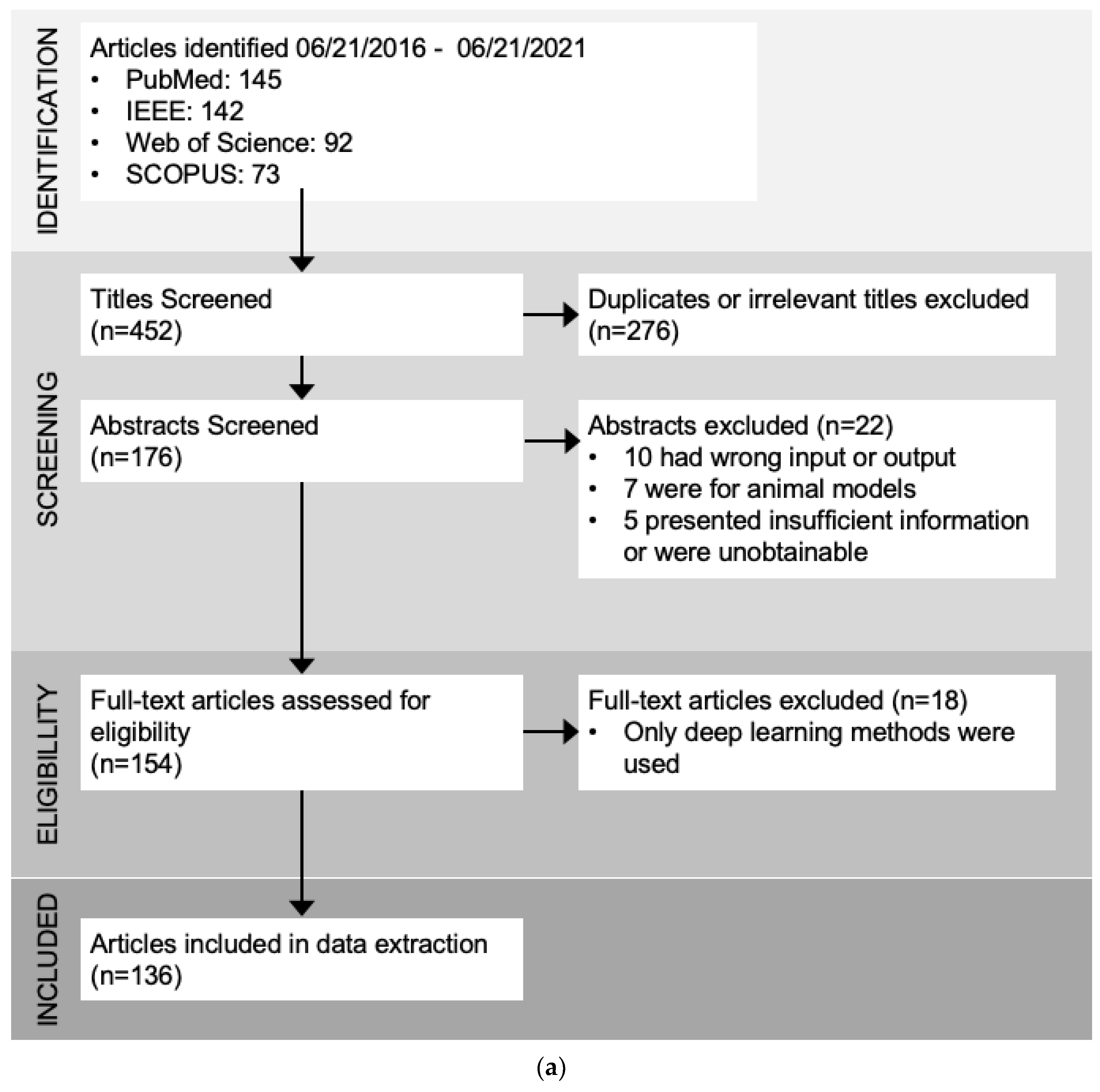
2. Methods
- Classification algorithm is not used on biomedical data or time series data;
- The article does not focus on classification algorithms, but regression algorithms, clustering algorithms, or other algorithms;
- The article focuses only on deep learning algorithms.
- No access to full paper;
- Not enough information about classification algorithm performance included;
- The data came from animals instead of humans;
- The algorithms used are not classification algorithms.
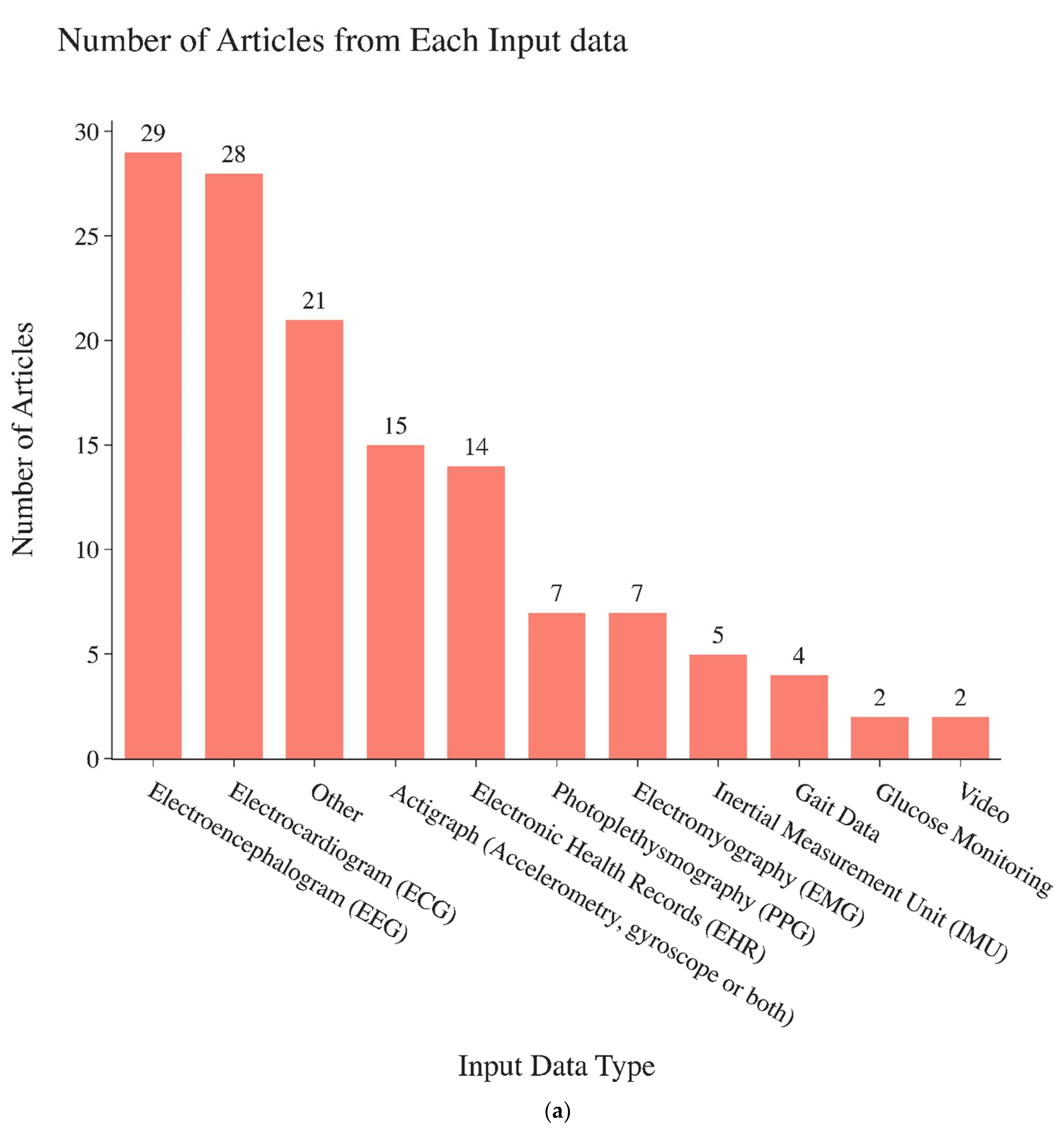
3. Results
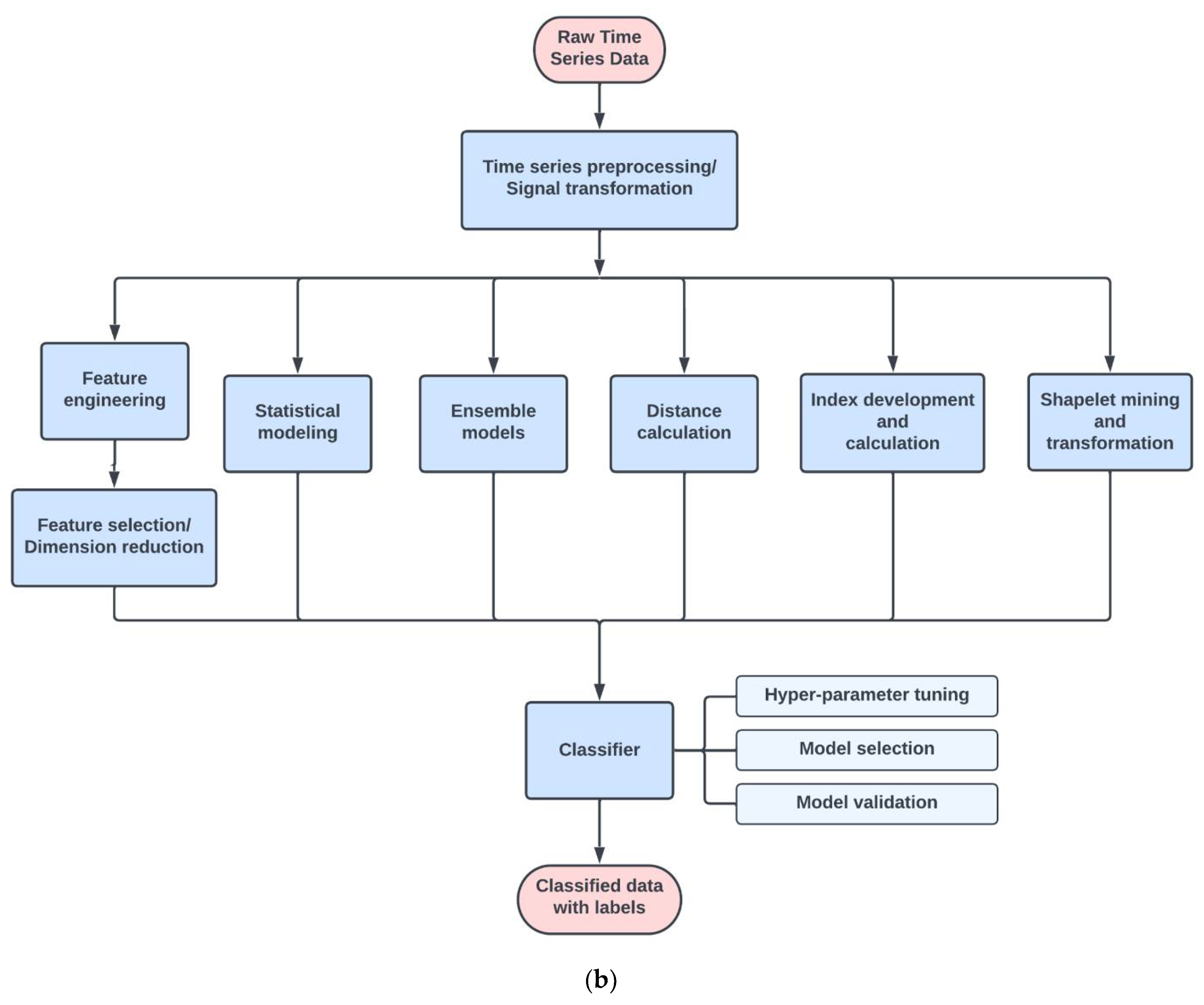
4. Algorithm Summaries
4.1. Preprocessing Methods
4.2. Feature Engineering Methods
- Preprocessing: this step takes raw data as the input and performs some manipulation of the data to return cleaner signals. Common steps include artifact removal, filtering, and segmentation.
- Signal transformation: this step can be used in preprocessing and also as a precursor to feature extraction. Some manipulation is performed on the signal to represent it in a different space. Common choices are Fourier Transform and wavelet transforms.
- Feature extraction: in this step, features are extracted from the time series data as a new representation of the original time series.
- Feature selection: this step selects the features that are the most descriptive, or have the most explanation power. Feature selection is also frequently performed in conjunction with model building.
- Model selection: the best model is found through hyperparameter tuning and/or comparisons between different types of algorithms.
- Model validation: performance metrics are calculated for all of the final models. This is frequently done in conjunction with model selection and often using some form of cross-validation.
4.3. Other Methods
4.4. Interpretation Methods
4.5. Best Performing Algorithms
5. Discussion
5.1. Small Datasets
5.2. Clinical Decision Support
5.3. Medical Devices
6. Limitations
7. Conclusions
Supplementary Materials
Author Contributions
Funding
Institutional Review Board Statement
Informed Consent Statement
Data Availability Statement
Acknowledgments
Conflicts of Interest
References
- Bock, C.; Moor, M.; Jutzeler, C.R.; Borgwardt, K. Machine Learning for Biomedical Time Series Classification: From Shapelets to Deep Learning. In Artificial Neural Networks; Cartwright, H., Ed.; Springer: New York, NY, USA, 2021; pp. 33–71. [Google Scholar] [CrossRef]
- Fawaz, H.I.; Forestier, G.; Weber, J.; Idoumghar, L.; Muller, P.-A. Deep learning for time series classification: A review. Data Min. Knowl. Discov. 2019, 33, 917–963. [Google Scholar] [CrossRef]
- Li, Y.; Tang, X.; Wang, A.; Tang, H. Probability density distribution of delta RR intervals: A novel method for the detection of atrial fibrillation. Australas. Phys. Eng. Sci. Med. 2017, 40, 707–716. [Google Scholar] [CrossRef] [PubMed]
- García-Martínez, B.; Martínez-Rodrigo, A.; Fernández-Caballero, A.; Moncho-Bogani, J.; Alcaraz, R. Nonlinear predictability analysis of brain dynamics for automatic recognition of negative stress. Neural Comput. Appl. 2018, 32, 13221–13231. [Google Scholar] [CrossRef]
- Tabar, Y.R.; Mikkelsen, K.B.; Rank, M.L.; Hemmsen, M.C.; Kidmose, P. Investigation of low dimensional feature spaces for automatic sleep staging. Comput. Methods Programs Biomed. 2021, 205, 106091. [Google Scholar] [CrossRef] [PubMed]
- Smartwatch penetration 2020. Statista. Available online: https://www.statista.com/statistics/1107874/access-to-smartwatch-in-households-worldwide/ (accessed on 25 July 2022).
- Xie, J.; Wen, D.; Liang, L.; Jia, Y.; Gao, L.; Lei, J. Evaluating the Validity of Current Mainstream Wearable Devices in Fitness Tracking Under Various Physical Activities: Comparative Study. JMIR mHealth uHealth 2018, 6, e94. [Google Scholar] [CrossRef] [PubMed]
- Guillodo, E.; Lemey, C.; Simonnet, M.; Walter, M.; Baca-García, E.; Masetti, V.; Moga, S.; Larsen, M.; Network, H.; Ropars, J.; et al. Clinical Applications of Mobile Health Wearable–Based Sleep Monitoring: Systematic Review. JMIR mHealth uHealth 2020, 8, e10733. [Google Scholar] [CrossRef] [PubMed]
- Bet, P.; Castro, P.C.; Ponti, M. Fall detection and fall risk assessment in older person using wearable sensors: A systematic review. Int. J. Med. Informatics 2019, 130, 103946. [Google Scholar] [CrossRef]
- Turakhia, M.P.; Desai, M.; Hedlin, H.; Rajmane, A.; Talati, N.; Ferris, T.; Desai, S.; Nag, D.; Patel, M.; Kowey, P.; et al. Rationale and design of a large-scale, app-based study to identify cardiac arrhythmias using a smartwatch: The Apple Heart Study. Am. Hear. J. 2018, 207, 66–75. [Google Scholar] [CrossRef] [PubMed]
- Marcus, G. Deep Learning: A Critical Appraisal. arXiv 2018, arXiv:1801.00631. [Google Scholar]
- Fisher, A.J.; Medaglia, J.D.; Jeronimus, B.F. Lack of group-to-individual generalizability is a threat to human subjects research. Proc. Natl. Acad. Sci. USA 2018, 115, E6106–E6115. [Google Scholar] [CrossRef]
- Ruiz, A.P.; Flynn, M.; Large, J.; Middlehurst, M.; Bagnall, A. The great multivariate time series classification bake off: A review and experimental evaluation of recent algorithmic advances. Data Min. Knowl. Discov. 2020, 35, 401–449. [Google Scholar] [CrossRef] [PubMed]
- Hossin, M.; Sulaiman, M.N. A Review on Evaluation Metrics for Data Classification Evaluations. Int. J. Data Min. Knowl. Manag. Process 2015, 5, 1–11. [Google Scholar] [CrossRef]
- Davis, J.; Goadrich, M. The relationship between Precision-Recall and ROC curves. In Proceedings of the 23rd International Conference on Machine Learning, New York, NY, USA, 25–29 June 2006; pp. 233–240. [Google Scholar] [CrossRef]
- The Elements of Statistical Learning. Available online: http://link.springer.com/book/10.1007/978-0-387-84858-7 (accessed on 14 August 2022).
- Hidden Markov Model. Wikipedia. 18 July 2022. Available online: https://en.wikipedia.org/w/index.php?title=Hidden_Markov_model&oldid=1098931761 (accessed on 14 August 2022).
- Talebi, S. The Wavelet Transform. Medium. 8 January 2021. Available online: https://towardsdatascience.com/the-wavelet-transform-e9cfa85d7b34 (accessed on 13 February 2022).
- Regan, M. K Nearest Neighbors & Dynamic Time Warping. 3 August 2022. Available online: https://github.com/markdregan/K-Nearest-Neighbors-with-Dynamic-Time-Warping (accessed on 14 August 2022).
- Figure 10: Using the Gaussian Mixture Model to Estimate the Threshold. ResearchGate. Available online: https://www.researchgate.net/figure/Using-the-Gaussian-Mixture-Model-to-Estimate-the-Threshold_fig4_307984756 (accessed on 14 August 2022).
- Sokolova, M.; Japkowicz, N.; Szpakowicz, S. Beyond Accuracy, F-Score and ROC: A Family of Discriminant Measures for Performance Evaluation. In AI 2006: Advances in Artificial Intelligence; Springer: Berlin/Heidelberg, Germany, 2006; pp. 1015–1021. [Google Scholar] [CrossRef]
- Luque, A.; Carrasco, A.; Martín, A.; de las Heras, A. The impact of class imbalance in classification performance metrics based on the binary confusion matrix. Pattern Recognit. 2019, 91, 216–231. [Google Scholar] [CrossRef]
- Mole, S.S.S.; Sujatha, K. An efficient Gait Dynamics classification method for Neurodegenerative Diseases using Brain signals. J. Med. Syst. 2019, 43, 245. [Google Scholar] [CrossRef] [PubMed]
- Joshi, D.; Khajuria, A.; Joshi, P. An automatic non-invasive method for Parkinson’s disease classification. Comput. Methods Programs Biomed. 2017, 145, 135–145. [Google Scholar] [CrossRef] [PubMed]
- Tor, H.T.; Ooi, C.P.; Lim-Ashworth, N.S.; Wei, J.K.E.; Jahmunah, V.; Oh, S.L.; Acharya, U.R.; Fung, D.S.S. Automated detection of conduct disorder and attention deficit hyperactivity disorder using decomposition and nonlinear techniques with EEG signals. Comput. Methods Programs Biomed. 2021, 200, 105941. [Google Scholar] [CrossRef]
- Mesbah, S.; Gonnelli, F.; Angeli, C.A.; El-Baz, A.; Harkema, S.J.; Rejc, E. Neurophysiological markers predicting recovery of standing in humans with chronic motor complete spinal cord injury. Sci. Rep. 2019, 9, 14474. [Google Scholar] [CrossRef] [PubMed]
- Anh, N.X.; Nataraja, R.; Chauhan, S. Towards near real-time assessment of surgical skills: A comparison of feature extraction techniques. Comput. Methods Progr. Biomed. 2019, 187, 105234. [Google Scholar] [CrossRef]
- Durongbhan, P.; Zhao, Y.; Chen, L.; Zis, P.; De Marco, M.; Unwin, Z.C.; Venneri, A.; He, X.; Li, S.; Zhao, Y.; et al. A Dementia Classification Framework Using Frequency and Time-Frequency Features Based on EEG Signals. IEEE Trans. Neural Syst. Rehabil. Eng. Publ. IEEE Eng. Med. Biol. Soc. 2019, 27, 826–835. [Google Scholar] [CrossRef]
- Bhattacharya, S.; Mazumder, O.; Roy, D.; Sinha, A.; Ghose, A. Synthetic Data Generation Through Statistical Explosion: Improving Classification Accuracy of Coronary Artery Disease Using PPG. In Proceedings of the ICASSP 2020–2020 IEEE International Conference on Acoustics, Speech and Signal Processing (ICASSP), Barcelona, Spain, 4–8 May 2020; pp. 1165–1169. [Google Scholar] [CrossRef]
- Walter, S.; Gruss, S.; Limbrecht-Ecklundt, K.; Traue, H.C.; Werner, P.; Al-Hamadi, A.; Diniz, N.; da Silva, G.M.; Andrade, A.O. Automatic pain quantification using autonomic parameters. Psychol. Neurosci. 2014, 7, 363–380. [Google Scholar] [CrossRef]
- Newman, J.L.; Phillips, J.S.; Cox, S.J.; FitzGerald, J.; Bath, A. Automatic nystagmus detection and quantification in long-term continuous eye-movement data. Comput. Biol. Med. 2019, 114, 103448. [Google Scholar] [CrossRef] [PubMed]
- Elsayed, N.; Maida, A.S.; Bayoumi, M. An Analysis of Univariate and Multivariate Electrocardiography Signal Classification. 2019, 396–399. In Proceedings of the 2019 18th IEEE International Conference On Machine Learning And Applications (ICMLA), Boca Raton, FL, USA, 16–19 December 2019; pp. 396–399. [Google Scholar] [CrossRef]
- She, X.; Zhai, Y.; Henao, R.; Woods, C.W.; Chiu, C.; Ginsburg, G.S.; Song, P.X.K.; Hero, A.O. Adaptive Multi-Channel Event Segmentation and Feature Extraction for Monitoring Health Outcomes. IEEE Trans. Biomed. Eng. 2020, 68, 2377–2388. [Google Scholar] [CrossRef] [PubMed]
- Garcia, H.F.; Alvarez, M.A.; Orozco, A.A. Gaussian process dynamical models for multimodal affect recognition. In Proceedings of the 2016 38th Annual International Conference of the IEEE Engineering in Medicine and Biology Society (EMBC), Orlando, FL, USA, 16–20 August 2016; pp. 850–853. [Google Scholar] [CrossRef]
- Zhou, P.-Y.; Chan, K.C.C. Fuzzy Feature Extraction for Multichannel EEG Classification. IEEE Trans. Cogn. Dev. Syst. 2016, 10, 267–279. [Google Scholar] [CrossRef]
- Forestier, G.; Petitjean, F.; Riffaud, L.; Jannin, P. Automatic matching of surgeries to predict surgeons’ next actions. Artif. Intell. Med. 2017, 81, 3–11. [Google Scholar] [CrossRef]
- Iscan, M.; Yigit, F.; Yilmaz, C. Heartbeat pattern classification algorithm based on Gaussian mixture model. In Proceedings of the 2016 IEEE International Symposium on Medical Measurements and Applications (MeMeA), Benevento, Italy, 15–18 May 2016; pp. 1–6. [Google Scholar] [CrossRef]
- Zhou, H.; Ji, N.; Samuel, O.W.; Cao, Y.; Zhao, Z.; Chen, S.; Li, G. Towards Real-Time Detection of Gait Events on Different Terrains Using Time-Frequency Analysis and Peak Heuristics Algorithm. Sensors 2016, 16, 1634. [Google Scholar] [CrossRef]
- Ji, N.; Zhou, H.; Guo, K.; Samuel, O.W.; Huang, Z.; Xu, L.; Li, G. Appropriate Mother Wavelets for Continuous Gait Event Detection Based on Time-Frequency Analysis for Hemiplegic and Healthy Individuals. Sensors 2019, 19, 3462. [Google Scholar] [CrossRef]
- Lu, L.; Mao, J.; Wang, W.; Ding, G.; Zhang, Z. A Study of Personal Recognition Method Based on EMG Signal. IEEE Trans. Biomed. Circuits Syst. 2020, 14, 681–691. [Google Scholar] [CrossRef]
- Liu, J.; Zhao, Y.; Lai, B.; Wang, H.; Tsui, K.L. Wearable Device Heart Rate and Activity Data in an Unsupervised Approach to Personalized Sleep Monitoring: Algorithm Validation. JMIR mHealth uHealth 2020, 8, e18370. [Google Scholar] [CrossRef]
- Cimbalnik, J.; Brinkmann, B.; Kremen, V.; Jurak, P.; Berry, B.; Van Gompel, J.; Stead, M.; Worrell, G. Physiological and pathological high frequency oscillations in focal epilepsy. Ann. Clin. Transl. Neurol. 2018, 5, 1062–1076. [Google Scholar] [CrossRef]
- Ren, H.; Ye, Z.; Li, Z. Anomaly detection based on a dynamic Markov model. Inf. Sci. 2017, 411, 52–65. [Google Scholar] [CrossRef]
- Elden, R.H.; Ghoneim, V.F.; Al-Atabany, W. A computer aided diagnosis system for the early detection of neurodegenerative diseases using linear and non-linear analysis. In Proceedings of the 2018 IEEE 4th Middle East Conference on Biomedical Engineering (MECBME), Tunis, Tunisia, 28–30 March 2018; pp. 116–121. [Google Scholar] [CrossRef]
- Heartbeat Classification Using Abstract Features From the Abductive Interpretation of the ECG|IEEE Journals & Magazine|IEEE Xplore. Available online: https://ieeexplore-ieee-org.proxy.lib.duke.edu/document/7750556 (accessed on 6 February 2022).
- Gupta, R.; Kundu, P. Dissimilarity factor based classification of inferior myocardial infarction ECG. In Proceedings of the 2016 IEEE First International Conference on Control, Measurement and Instrumentation (CMI), Kolkata, India, 8–10 January 2016; pp. 229–233. [Google Scholar] [CrossRef]
- Mohammadi-Ghazi, R.; Marzouk, Y.M.; Büyüköztürk, O. Conditional classifiers and boosted conditional Gaussian mixture model for novelty detection. Pattern Recognit. 2018, 81, 601–614. [Google Scholar] [CrossRef]
- Reamaroon, N.; Sjoding, M.W.; Lin, K.; Iwashyna, T.J.; Najarian, K. Accounting for Label Uncertainty in Machine Learning for Detection of Acute Respiratory Distress Syndrome. IEEE J. Biomed. Heal. Informatics 2018, 23, 407–415. [Google Scholar] [CrossRef] [PubMed]
- Park, G.H.; Kim, S.J.; Cho, Y.S. Development of a voiding diary using urination recognition technology in mobile environment. J. Exerc. Rehabil. 2020, 16, 529–533. [Google Scholar] [CrossRef] [PubMed]
- David, S.; Machado, J.; Inácio, C.; Valentim, C. A combined measure to differentiate EEG signals using fractal dimension and MFDFA-Hurst. Commun. Nonlinear Sci. Numer. Simul. 2020, 84, 105170. [Google Scholar] [CrossRef]
- Li, M.; Tian, S.; Sun, L.; Chen, X. Gait Analysis for Post-Stroke Hemiparetic Patient by Multi-Features Fusion Method. Sensors 2019, 19, 1737. [Google Scholar] [CrossRef]
- Gunnarsdottir, K.; Sadashivaiah, V.; Kerr, M.; Santaniello, S.; Sarma, S.V. Using demographic and time series physiological features to classify sepsis in the intensive care unit. In Proceedings of the 2016 38th Annual International Conference of the IEEE Engineering in Medicine and Biology Society (EMBC), Orlando, FL, USA, 16–20 August 2016; pp. 778–782. [Google Scholar] [CrossRef]
- Mertzanis, L.; Panotonoulou, A.; Skoularidou, M.; Kontoyiannis, I. Deep Tree Models for ‘Big’ Biological Data. In Proceedings of the 2018 IEEE 19th International Workshop on Signal Processing Advances in Wireless Communications (SPAWC), Kalamata, Greece, 25–28 June 2018; pp. 1–5. [Google Scholar] [CrossRef]
- El-Rashidy, N.; El-Sappagh, S.; Abuhmed, T.; Abdelrazek, S.M.; El-Bakry, H.M. Intensive Care Unit Mortality Prediction: An Improved Patient-Specific Stacking Ensemble Model. IEEE Access 2020, 8, 133541–133564. [Google Scholar] [CrossRef]
- Hong, S.; Kwon, H.; Choi, S.H.; Park, K.S. Intelligent system for drowsiness recognition based on ear canal electroencephalography with photoplethysmography and electrocardiography. Inf. Sci. 2018, 453, 302–322. [Google Scholar] [CrossRef]
- Nancy, J.Y.; Khanna, N.H.; Kannan, A. A bio-statistical mining approach for classifying multivariate clinical time series data observed at irregular intervals. Expert Syst. Appl. 2017, 78, 283–300. [Google Scholar] [CrossRef]
- Miao, B.; Guan, J.; Zhang, L.; Meng, Q.; Zhang, Y. Automated Epileptic Seizure Detection Method Based on the Multi-attribute EEG Feature Pool and mRMR Feature Selection Method. In Proceedings of the International Conference on Computational Science—ICCS 2019, Faro, Portugal, 12–14 June 2019; Rodrigues, J.M.F., Cardoso, P.J.S., Monteiro, J., Lam, R., Krzhizhanovskaya, V.V., Lees, M.H., Dongarra, J.J., Sloot, P.M.A., Eds.; Springer: Cham, Switzerland, 2019; Volume 11538, pp. 45–59. [Google Scholar] [CrossRef]
- Orphanou, K.; Dagliati, A.; Sacchi, L.; Stassopoulou, A.; Keravnou, E.; Bellazzi, R. Incorporating repeating temporal association rules in Naïve Bayes classifiers for coronary heart disease diagnosis. J. Biomed. Inform. 2018, 81, 74–82. [Google Scholar] [CrossRef]
- Lacson, R.C.; Baker, B.; Suresh, H.; Andriole, K.; Szolovits, P.; Lacson, E. Use of machine-learning algorithms to determine features of systolic blood pressure variability that predict poor outcomes in hypertensive patients. Clin. Kidney J. 2018, 12, 206–212. [Google Scholar] [CrossRef]
- Ozdenizci, O.; Cumpanasoiu, C.; Mazefsky, C.; Siegel, M.; Erdoğgmus, D.; Ioannidis, S.; Goodwin, M.S. Time-Series Prediction of Proximal Aggression Onset in Minimally-Verbal Youth with Autism Spectrum Disorder Using Physiological Biosignals. In Proceedings of the 2018 40th Annual International Conference of the IEEE Engineering in Medicine and Biology Society (EMBC), Honolulu, HI, USA, 18–21 July 2018; pp. 5745–5748. [Google Scholar] [CrossRef]
- Lotfan, S.; Shahyad, S.; Khosrowabadi, R.; Mohammadi, A.; Hatef, B. Support vector machine classification of brain states exposed to social stress test using EEG-based brain network measures. Biocybern. Biomed. Eng. 2018, 39, 199–213. [Google Scholar] [CrossRef]
- Ródenas, J.; García, M.; Alcaraz, R.; Rieta, J.J. Combined Nonlinear Analysis of Atrial and Ventricular Series for Automated Screening of Atrial Fibrillation. Complexity 2017, 2017, 2163610. [Google Scholar] [CrossRef]
- Cuesta-Frau, D.; Novák, D.; Burda, V.; Molina-Picó, A.; Vargas, B.; Mraz, M.; Kavalkova, P.; Benes, M.; Haluzik, M. Characterization of Artifact Influence on the Classification of Glucose Time Series Using Sample Entropy Statistics. Entropy 2018, 20, 871. [Google Scholar] [CrossRef] [PubMed]
- Zdravevski, E.; Lameski, P.; Trajkovik, V.; Kulakov, A.; Chorbev, I.; Goleva, R.; Pombo, N.; Garcia, N. Improving Activity Recognition Accuracy in Ambient-Assisted Living Systems by Automated Feature Engineering. IEEE Access 2017, 5, 5262–5280. [Google Scholar] [CrossRef]
- Peng, P.; Wei, H.; Xie, L.; Song, Y. Epileptic Seizure Prediction in Scalp EEG Using an Improved HIVE-COTE Model. In Proceedings of the 2020 39th Chinese Control Conference (CCC), Shenyang, China, 27–29 July 2020; pp. 6450–6457. [Google Scholar] [CrossRef]
- Li, X.; Zhang, Y.; Jiang, F.; Zhao, H. A novel machine learning unsupervised algorithm for sleep/wake identification using actigraphy. Chronobiol. Int. 2020, 37, 1002–1015. [Google Scholar] [CrossRef] [PubMed]
- Bragança, H.; Colonna, J.G.; Lima, W.S.; Souto, E. A Smartphone Lightweight Method for Human Activity Recognition Based on Information Theory. Sensors 2020, 20, 1856. [Google Scholar] [CrossRef]
- Pham, M.H.; Elshehabi, M.; Haertner, L.; Del Din, S.; Srulijes, K.; Heger, T.; Synofzik, M.; Hobert, M.A.; Faber, G.S.; Hansen, C.; et al. Validation of a Step Detection Algorithm during Straight Walking and Turning in Patients with Parkinson’s Disease and Older Adults Using an Inertial Measurement Unit at the Lower Back. Front. Neurol. 2017, 8, 457. [Google Scholar] [CrossRef]
- Ivaturi, P.; Gadaleta, M.; Pandey, A.C.; Pazzani, M.; Steinhubl, S.R.; Quer, G. A Comprehensive Explanation Framework for Biomedical Time Series Classification. IEEE J. Biomed. Health Inform. 2021, 25, 2398–2408. [Google Scholar] [CrossRef]
- Adam, M.; Oh, S.L.; Sudarshan, V.K.; Koh, J.E.; Hagiwara, Y.; Tan, J.H.; Tan, R.S.; Acharya, U.R. Automated characterization of cardiovascular diseases using relative wavelet nonlinear features extracted from ECG signals. Comput. Methods Programs Biomed. 2018, 161, 133–143. [Google Scholar] [CrossRef]
- He, R.; Wang, K.; Zhao, N.; Liu, Y.; Yuan, Y.; Li, Q.; Zhang, H. Automatic Detection of Atrial Fibrillation Based on Continuous Wavelet Transform and 2D Convolutional Neural Networks. Front. Physiol. 2018, 9, 1206. [Google Scholar] [CrossRef]
- Ugur, T.K.; Erdamar, A. An efficient automatic arousals detection algorithm in single channel EEG. Comput. Methods Programs Biomed. 2019, 173, 131–138. [Google Scholar] [CrossRef] [PubMed]
- Casado, F.E.; Rodríguez, G.; Iglesias, R.; Regueiro, C.V.; Barro, S.; Canedo-Rodríguez, A. Walking Recognition in Mobile Devices. Sensors 2020, 20, 1189. [Google Scholar] [CrossRef] [PubMed]
- Islam, R.; Pavel, S.R.; Tunaz, S.A. Neurodegenerative Disease Classification Using Gait Signal Features and Random Forest Classifier. In Proceedings of the 2019 4th International Conference on Electrical Information and Communication Technology, (EICT), Khulna, Bangladesh, 20–22 December 2019; pp. 1–4. [Google Scholar] [CrossRef]
- Hemmati, S.; Wade, E. Detecting postural transitions: A robust wavelet-based approach. In Proceedings of the 2016 38th Annual International Conference of the IEEE Engineering in Medicine and Biology Society (EMBC), Orlando, FL, USA, 16–20 August 2016; pp. 3704–3707. [Google Scholar] [CrossRef]
- Martindale, C.F.; Hoenig, F.; Strohrmann, C.; Eskofier, B.M. Smart Annotation of Cyclic Data Using Hierarchical Hidden Markov Models. Sensors 2017, 17, 2328. [Google Scholar] [CrossRef] [PubMed]
- Canbek, G.; Temizel, T.T.; Sagiroglu, S. BenchMetrics: A systematic benchmarking method for binary classification performance metrics. Neural Comput. Appl. 2021, 33, 14623–14650. [Google Scholar] [CrossRef]
- Bent, B.; Wang, K.; Grzesiak, E.; Jiang, C.; Qi, Y.; Jiang, Y.; Cho, P.; Zingler, K.; Ogbeide, F.I.; Zhao, A.; et al. The digital biomarker discovery pipeline: An open-source software platform for the development of digital biomarkers using mHealth and wearables data. J. Clin. Transl. Sci. 2020, 5. [Google Scholar] [CrossRef] [PubMed]
- Shi, Y.; Li, F.; Liu, T.; Beyette, F.R.; Song, W. Dynamic Time-frequency Feature Extraction for Brain Activity Recognition. In Proceedings of the 2018 40th Annual International Conference of the IEEE Engineering in Medicine and Biology Society (EMBC), Honolulu, HI, USA, 18–21 July 2018; pp. 3104–3107. [Google Scholar] [CrossRef]
- Zarei, A.; Asl, B.M. Automatic Detection of Obstructive Sleep Apnea Using Wavelet Transform and Entropy-Based Features From Single-Lead ECG Signal. IEEE J. Biomed. Health Inform. 2018, 23, 1011–1021. [Google Scholar] [CrossRef]
- Liu, L.; Wang, H.; Li, H.; Liu, J.; Qiu, S.; Zhao, H.; Guo, X. Ambulatory Human Gait Phase Detection Using Wearable Inertial Sensors and Hidden Markov Model. Sensors 2021, 21, 1347. [Google Scholar] [CrossRef]
- Zhang, C.; Chen, Y.; Yin, A.; Wang, X. Anomaly detection in ECG based on trend symbolic aggregate approximation. Math. Biosci. Eng. 2019, 16, 2154–2167. [Google Scholar] [CrossRef]
- Lee, S.X.; Leemaqz, S.Y. Automated Wrist Pulse diagnosis of Pancreatitis via Autoregressive Discriminant Models. 2017, pp. 1262–1266. Available online: https://www.scopus.com/inward/record.uri?eid=2-s2.0-85080915306&partnerID=40&md5=f92bd168c60aae1a6ffbda888f5663f0 (accessed on 15 August 2022).
- Bagattini, F.; Karlsson, I.; Rebane, J.; Papapetrou, P. A classification framework for exploiting sparse multi-variate temporal features with application to adverse drug event detection in medical records. BMC Med Informatics Decis. Mak. 2019, 19, 7. [Google Scholar] [CrossRef]
- Campbell, E.; Phinyomark, A.; Scheme, E. Feature Extraction and Selection for Pain Recognition Using Peripheral Physiological Signals. Front. Neurosci. 2019, 13, 437. [Google Scholar] [CrossRef]
- Jovic, A.; Brkic, K.; Krstacic, G. Detection of congestive heart failure from short-term heart rate variability segments using hybrid feature selection approach. Biomed. Signal Process. Control 2019, 53, 101583. [Google Scholar] [CrossRef]
- Nawaz, R.; Cheah, K.H.; Nisar, H.; Yap, V.V. Comparison of different feature extraction methods for EEG-based emotion recognition. Biocybern. Biomed. Eng. 2020, 40, 910–926. [Google Scholar] [CrossRef]
- Haddi, Z.; Ananou, B.; Trardi, Y.; Ouladsine, M.; Pons, J.-F.; Delliaux, S.; Deharo, J.-C. Relevance Vector Machine as Data-Driven Method for Medical Decision Making. In Proceedings of the 2019 18th European Control Conference (ECC), Naples, Italy, 25–28 June 2019; pp. 1011–1016. [Google Scholar] [CrossRef]
- Wickramasuriya, D.S.; Tessmer, M.K.; Faghih, R.T. Facial Expression-Based Emotion Classification using Electrocardiogram and Respiration Signals. In Proceedings of the 2019 IEEE Healthcare Innovations and Point of Care Technologies (HI-POCT), Bethesda, MD, USA, 20–22 November 2019; pp. 9–12. [Google Scholar] [CrossRef]
- Malik, A.R.; Boger, J. Zero-Effort Ambient Heart Rate Monitoring Using Ballistocardiography Detected Through a Seat Cushion: Prototype Development and Preliminary Study. JMIR Rehabilitation Assist. Technol. 2021, 8, e25996. [Google Scholar] [CrossRef] [PubMed]
- Liu, N.; Sun, M.; Wang, L.; Zhou, W.; Dang, H.; Zhou, X. A support vector machine approach for AF classification from a short single-lead ECG recording. Physiol. Meas. 2018, 39, 064004. [Google Scholar] [CrossRef] [PubMed]
- Goshvarpour, A. Evaluation of Novel Entropy-Based Complex Wavelet Sub-bands Measures of PPG in an Emotion Recognition System. J. Med. Biol. Eng. 2020, 40, 451–461. [Google Scholar] [CrossRef]
- Kolodziej, M.; Majkowski, A.; Rak, R.J.; Rysz, A.; Marchel, A. Decision Support System For Epileptogenic Zone Location during Brain Resection. Metrol. Meas. Syst. 2018, 25, 15–32. [Google Scholar] [CrossRef]
- Hu, Y.; An, W.; Subramanian, R.; Zhao, N.; Gu, Y.; Wu, W. Faster Clinical Time Series Classification with Filter Based Feature Engineering Tree Boosting Methods; Springer: Cham, Switzerland, 2021; Volume 914, p. 260. [Google Scholar] [CrossRef]
- Mumtaz, W.; Xia, L.; Yasin, M.A.M.; Ali, S.S.A.; Malik, A.S. A wavelet-based technique to predict treatment outcome for Major Depressive Disorder. PLoS ONE 2017, 12, e0171409. [Google Scholar] [CrossRef]


| Categories | Choices/Sub-Fields | Definitions/Descriptions |
|---|---|---|
| General (Relevant) Information | Article Type | The type of article for a particular paper being reviewed, such as Journal Article/Conference Article/Review Paper |
| Area of application | Describes the area of biomedical signal and application this paper is about. | |
| Aim of study | Defines the specific challenge or question this paper is aimed at tackling | |
| Name of Publisher/Journal/Conference | Site of article publication. | |
| Classification Task | Defines the kind of classification task performed in this article. (Pointwise classification, window classification, or whole sequence classification) | |
| Input data (X) | The type of input biomedical time series data | |
| Label (Y) | The output label or variable. Example: sleep vs wake, healthy vs diseased. | |
| Data source or open dataset name | States if the data are open source and where the dataset is hosted. | |
| Population Size | The number of subjects are included in this dataset. | |
| Data exclusion criteria | States the criteria considered to exclude subjects or specific parts of the data. | |
| All algorithms tested | List (or examples) of all the algorithms tested. | |
| Best algorithm name | The name of the best algorithm. | |
| Classification Task | Whole-Series Classification | In whole time series classification (WSC) for a dataset of n samples, we are provided a set of tuples where each of an entire time series is associated with one class label. |
| Sequence-to-sequence (point-wise) | The class label of each point in time is predicted. | |
| Window-based Classification or Onset Detection | Onset detection is a subtype of time series classification in which—as opposed to whole series classification—class labels are provided with a time-stamp. As an alternative to time pointwise classification, time-stamped labels have been leveraged for classifying time series windows that precede the class label’s time-stamp. For onset detection, a class label requires a time-stamp. This additional information can enforce that solely information from the past and present is used to predict a future target. This can be understood as a compromise between time pointwise classification and whole time series classification. An example is to detect the onset of sepsis in the intensive care unit | |
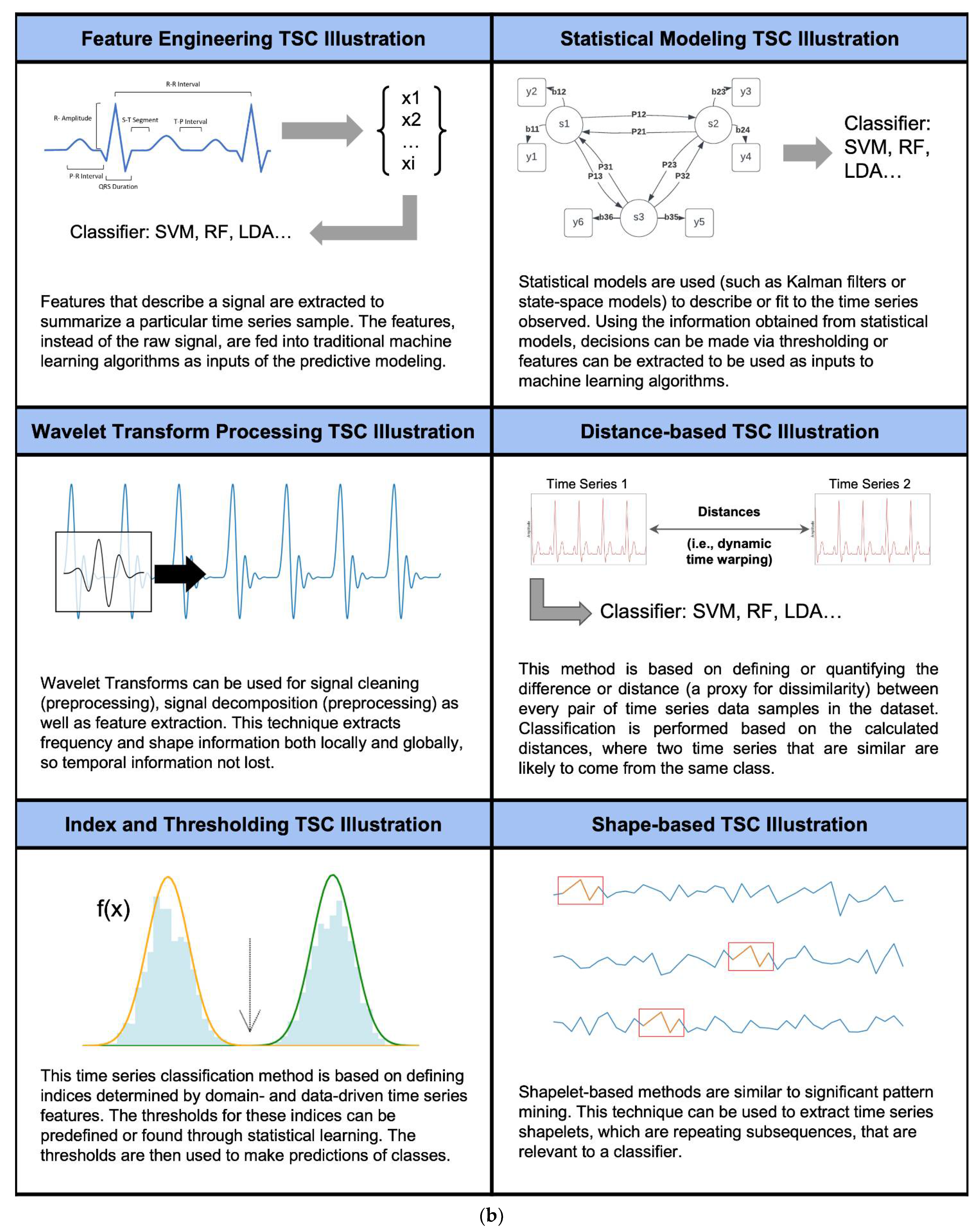
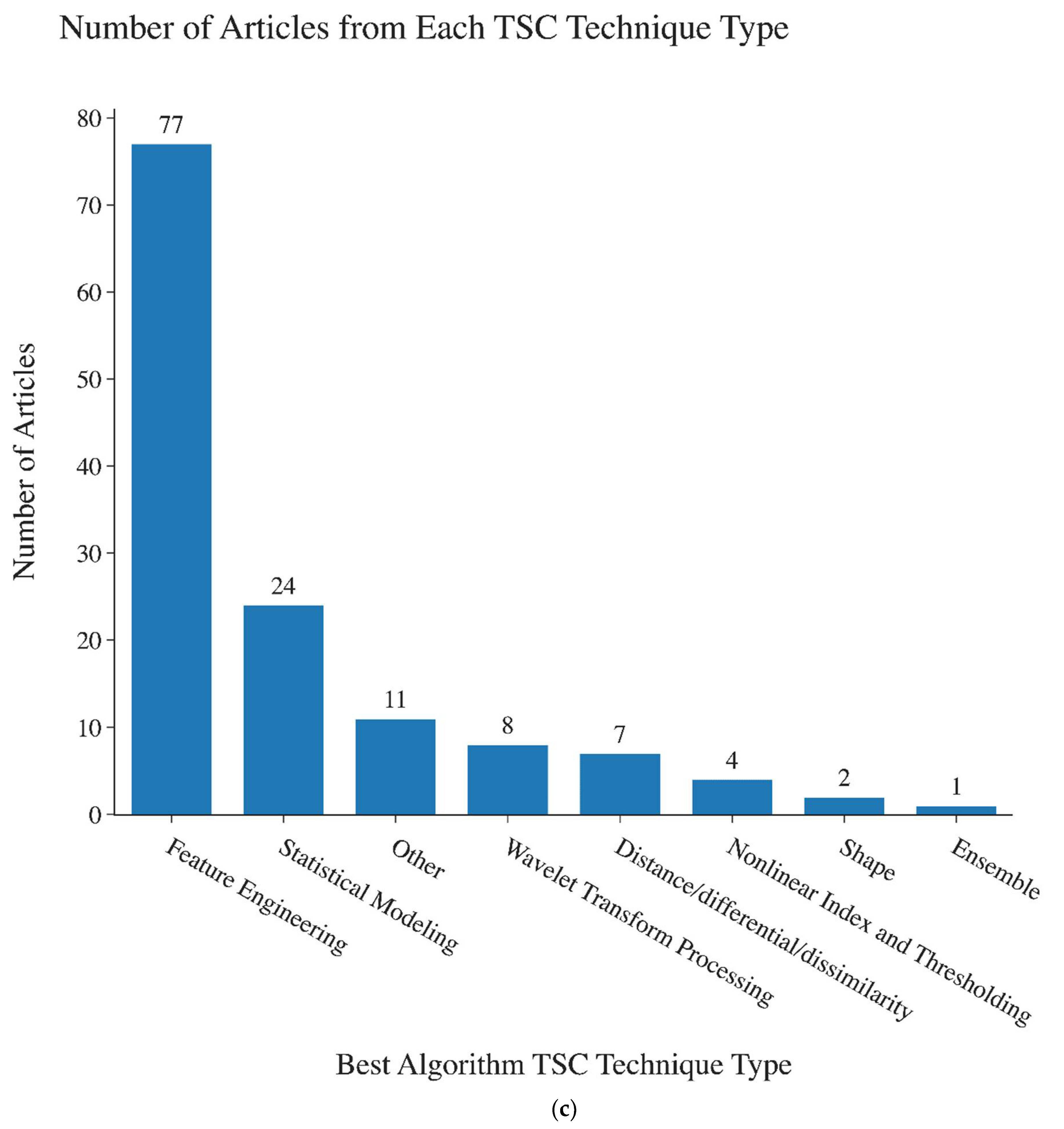
| Best Algorithm Class | Feature Engineering | The type of time series classification technique where features are extracted to describe a particular time series sample and the features are fed into traditional machine learning algorithms as inputs of the predictive modeling. |
| Statistical Modeling | This technique uses statistical modeling (such as Kalman filters or state-space models like Hidden Markov Models) to describe or fit the time series observed. Using the information obtained from statistical models, we can make decisions or extract features to be used as inputs to machine learning algorithms. | |
| Wavelet Transform [8] | Wavelet Transform can be used for signal cleaning (preprocessing), signal decomposition (preprocessing), and feature extraction. This technique is widely used and can be considered an integral part of time series machine learning. | |
| Distance-based methods [7] | This method is based on defining or quantifying the difference or distance (proxy for dissimilarity) between every pair of time series data samples in the dataset. Classification is performed based on the calculated distances, where two time series that are in close proximity (i.e., they have a small distance) under some distance measure are likely to come from the same class. | |
| Ensemble-based | Ensemble-based classification algorithms utilize multiple algorithms to make predictions and then aggregate the results coming from these different algorithms | |
| Shapelet/Shape-based | Shapelet-based methods are similar to significant pattern mining. Time series shapelets are subsequences that maximize classification performance. | |
| Non-linear index and thresholding | This time series classification method is based on defining indices based on domain- and data-driven time series features. The thresholds for these indices can be predefined or found through statistical learning. The thresholds are then used to make predictions of classes. | |
| Other | Any other methods of time series classification that cannot be easily categorized. | |
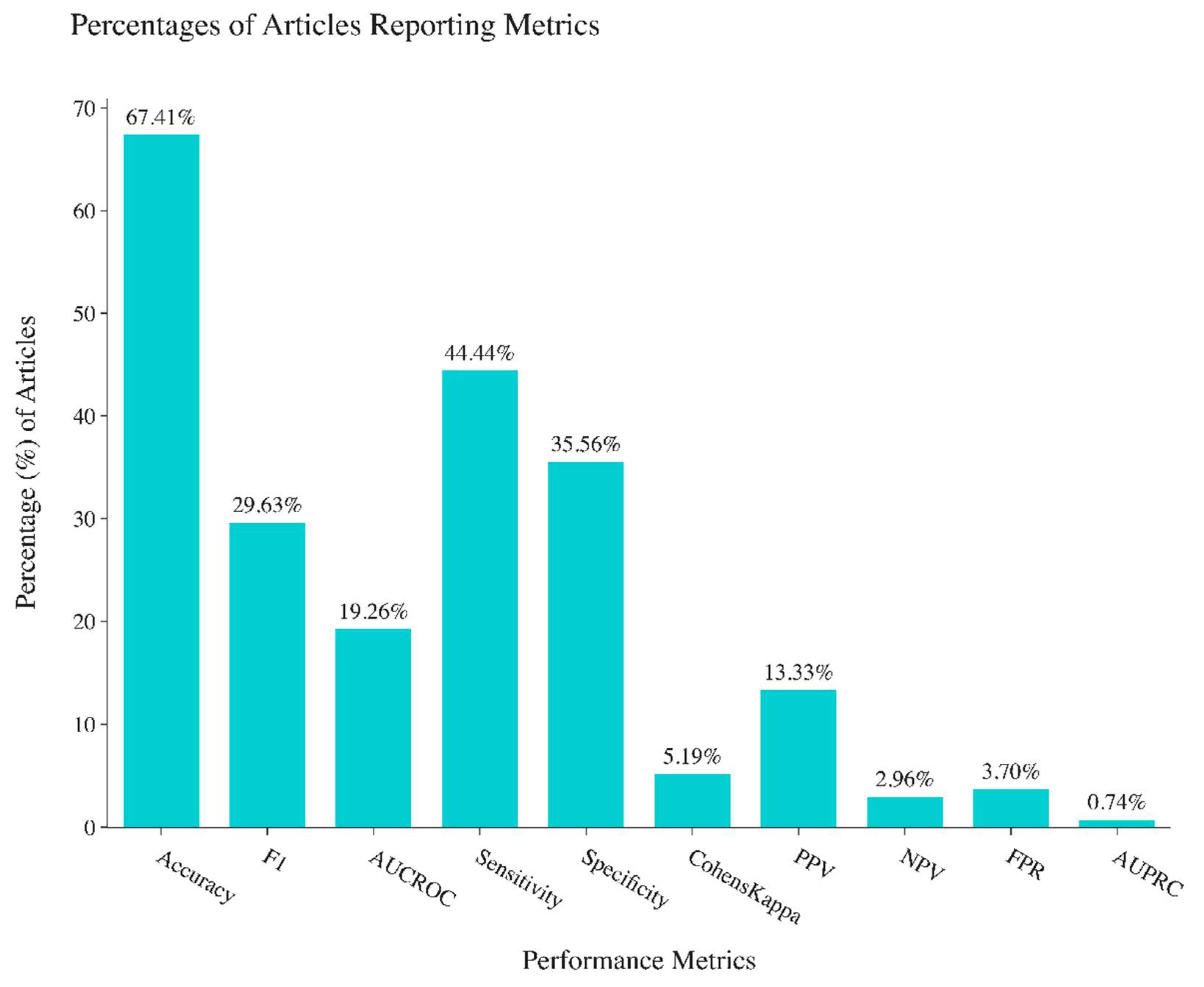
| Best Algorithm Performances [14,15] | Accuracy | The degree of correctness of a calculation of the best algorithm reported. |
| F1-score | The harmonic mean of precision and recall of the best algorithm reported. | |
| Area Under Curve of Receiver-Operating Characteristic | The measure of the usefulness of a test, in general, of the best algorithm reported. | |
| Sensitivity | The percentage of true positives of the best algorithm reported. | |
| Specificity | The percentage of true negatives of the best algorithm reported. | |
| Cohen’s Kappa | A statistical measure of inter-rater reliability for categorical variables of the best algorithm reported. | |
| Positive Predictive Value | The percentage of positive test results is a true positive. | |
| Negative Predictive Value | The percentage of negative test results is a true negative. | |
| False Positive Rate | The percentage of false alarm of the best algorithm reported | |
| Area Under Precision-Recall Curve | A model performance metric for binary responses that is appropriate for rare events and not dependent on model specificity |
| Type of Interpretation Method | Description | Example Papers |
|---|---|---|
| Plotting and Annotating Raw Signal | Plotting and annotating raw signals is a widely adopted and useful method for explaining the significance of differentiating features or shapes in time series classification problems. The plots generally consist of a representation of the raw or preprocessed signals in scatter or line plots and highlight the characteristics of the raw or transformed signal, which serves as the differentiating features or shapes for different classes. Some groups have also adopted plotting of preprocessed and transformed signals to present interpretable results. Examples of this method include plotting heart rate values with steps that compare rest and active periods, plotting detected anomalous sequences that are compared against normal sequences, and plotting time series samples in cluster plots after dimension reduction or feature extraction. | [41,42,43,44,45,46] |
| Visualization of indices over biological/physiological constructs | Instead of plotting against raw signals in 1D, researchers also routinely plot calculated or estimated metrics against 2D or 3D biological constructs, especially when the time series data are signals that represent complicated biological systems, such as brain activities or blood circulation. This interpretation method is very commonly used on electroencephalogram datasets, and examples include a graphical representation of the brain for mean calculated metrics for calm and distressed individuals, as well as a construction of 2D maps of scalp topographies that indicate statistical differences. | [4,26,28,47] |
| Statistical Analysis/Modeling | Statistical analysis and modeling are used to provide interpretability for not just the models built for classification, but also for clinical application and biomedical understanding. Various plots and tests can be used to demonstrate the relationship between outcomes and certain features or estimated metrics. Example plots are kernel distribution plots, distribution box-plots from statistical models, normality plots, and the visualization of the separability of indices through plotting of the index space. Example analysis tests include variance analysis, normality tests, correlation analysis, and also modeling techniques such as generalized linear models, bivariate random-effects models, and Bayesian hierarchical models. | [26,41,48,49,50,51,52,53] |
| Feature weight/importance analysis/ranking | Analysis and visualization of feature importance in a model are very helpful for researchers and clinicians to identify the most useful and important features that contribute to predicting an outcome or influencing a diagnosis. Many time series classification algorithms have built-in methods for feature importance analysis, such as Random Forest, Logistic Regression, and some statistical modeling based classification algorithms. In the pipeline of feature engineering techniques of time series classification, it is often seen that feature selection or dimension reduction are used, and these steps also automatically generate a ranking of feature importance to model building. Additionally, feature importance and ranking can be generated by specific techniques such as Fisher Importance score and Shapley values. | [44,54,55,56,57,58,59,60] |
| Classifier Boundary Plotted against features | Plotting the classifier’s boundary in the feature space or lower dimensional space helps to visualize the classifier’s ability to differentiate observations from one class to another, i.e., separability. SVM-based classifiers commonly utilize this method for interpretability. | [61] |
| Index Parameter and Threshold Tuning | Index parameter and threshold tuning is an interpretation method that is usually used in conjunction with classifier building by using a domain-driven approach. Using a domain-driven approach, the researchers typically try to design an index to quantify a biological or physiological phenomenon. The design of the index is usually flexible and can be tuned by changing the parameters used in the index’s formula. The threshold of the index is used to differentiate the classes (such as normal vs abnormal conditions, positive vs negative diagnosis). Both the parameters and the threshold of the designed index can be tuned using the existing the dataset, and the classifier’s performance metrics can be examined to find the best set of parameters and threshold(s) to achieve the best classifier performances. These parameters and thresholds could also have biomedical significance and meaning relevant for future medical understanding and research. Index analysis can be performed against record length (length of time series), missingness, sample saturation, and time offset. | [51,57,62,63] |
| Channel or Signal Selection | Channel or signal selection is a model building technique but also an interpretation method. Given the prevalence of multivariable time series data in biomedical applications, it is critical for researchers to determine which signals among many, or which channels, can be used for classification. By comparing the classifiers’ performances using different signals/channels or specifications of the signals (such as where the sensors are placed), researchers are able to find the best combination that achieves the best performance results, and hence provides interpretability in terms of which signal types or channels are most important for the given biomedical application. | [64,65,66] |
| Performance Comparisons Investigating Different Scenarios | Comparing classifier performance metrics when built under different scenarios serves as an interpretation method as well as an experimentation method. Experts in a domain of interest can make sense of why a certain scenario produces the best predictability or algorithm performance, thereby contributing to biomedical understanding and research. For example, accuracy and F1-scores can be compared using datasets collected under different sensor inputs, different user locations, different symbolic or discretization methods, and different data fusion techniques | [60,67] |
| Bland–Altman plot illustrating the agreement | Bland–Altman plots can be used to evaluate the difference between estimated predictions from the algorithm and the gold standard, thereby providing interpretation of the algorithm’s prediction power and potential usefulness as a digital biomarker. | [68] |
| Deep Learning Network Analysis | Although deep learning models are generally thought of as black box models without easy and direct insight into what the models are doing, there has been recent and impactful research into developing the interpretability of deep learning models and some methods for model explanation. The cited example paper introduces a “global and local explanation”. Global explanation means looking at entire classes of data that show which regions of the signal patterns have the most influence for a specific class. Local explanation is the analysis of specific input signals and model outcomes. These methods enable a deeper understanding of the network’s behavior, thereby showing the most informative regions that trigger the classification decision and highlighting the possible causes of abnormal physiology or behavior. | [69] |
Publisher’s Note: MDPI stays neutral with regard to jurisdictional claims in published maps and institutional affiliations. |
© 2022 by the authors. Licensee MDPI, Basel, Switzerland. This article is an open access article distributed under the terms and conditions of the Creative Commons Attribution (CC BY) license (https://creativecommons.org/licenses/by/4.0/).
Share and Cite
Wang, W.K.; Chen, I.; Hershkovich, L.; Yang, J.; Shetty, A.; Singh, G.; Jiang, Y.; Kotla, A.; Shang, J.Z.; Yerrabelli, R.; et al. A Systematic Review of Time Series Classification Techniques Used in Biomedical Applications. Sensors 2022, 22, 8016. https://doi.org/10.3390/s22208016
Wang WK, Chen I, Hershkovich L, Yang J, Shetty A, Singh G, Jiang Y, Kotla A, Shang JZ, Yerrabelli R, et al. A Systematic Review of Time Series Classification Techniques Used in Biomedical Applications. Sensors. 2022; 22(20):8016. https://doi.org/10.3390/s22208016
Chicago/Turabian StyleWang, Will Ke, Ina Chen, Leeor Hershkovich, Jiamu Yang, Ayush Shetty, Geetika Singh, Yihang Jiang, Aditya Kotla, Jason Zisheng Shang, Rushil Yerrabelli, and et al. 2022. "A Systematic Review of Time Series Classification Techniques Used in Biomedical Applications" Sensors 22, no. 20: 8016. https://doi.org/10.3390/s22208016
APA StyleWang, W. K., Chen, I., Hershkovich, L., Yang, J., Shetty, A., Singh, G., Jiang, Y., Kotla, A., Shang, J. Z., Yerrabelli, R., Roghanizad, A. R., Shandhi, M. M. H., & Dunn, J. (2022). A Systematic Review of Time Series Classification Techniques Used in Biomedical Applications. Sensors, 22(20), 8016. https://doi.org/10.3390/s22208016