
Investigation of a Sparse Autoencoder-Based Feature Transfer Learning Framework for Hydrogen Monitoring Using Microfluidic Olfaction Detectors

 ,
,  and
and 
Abstract
1. Introduction
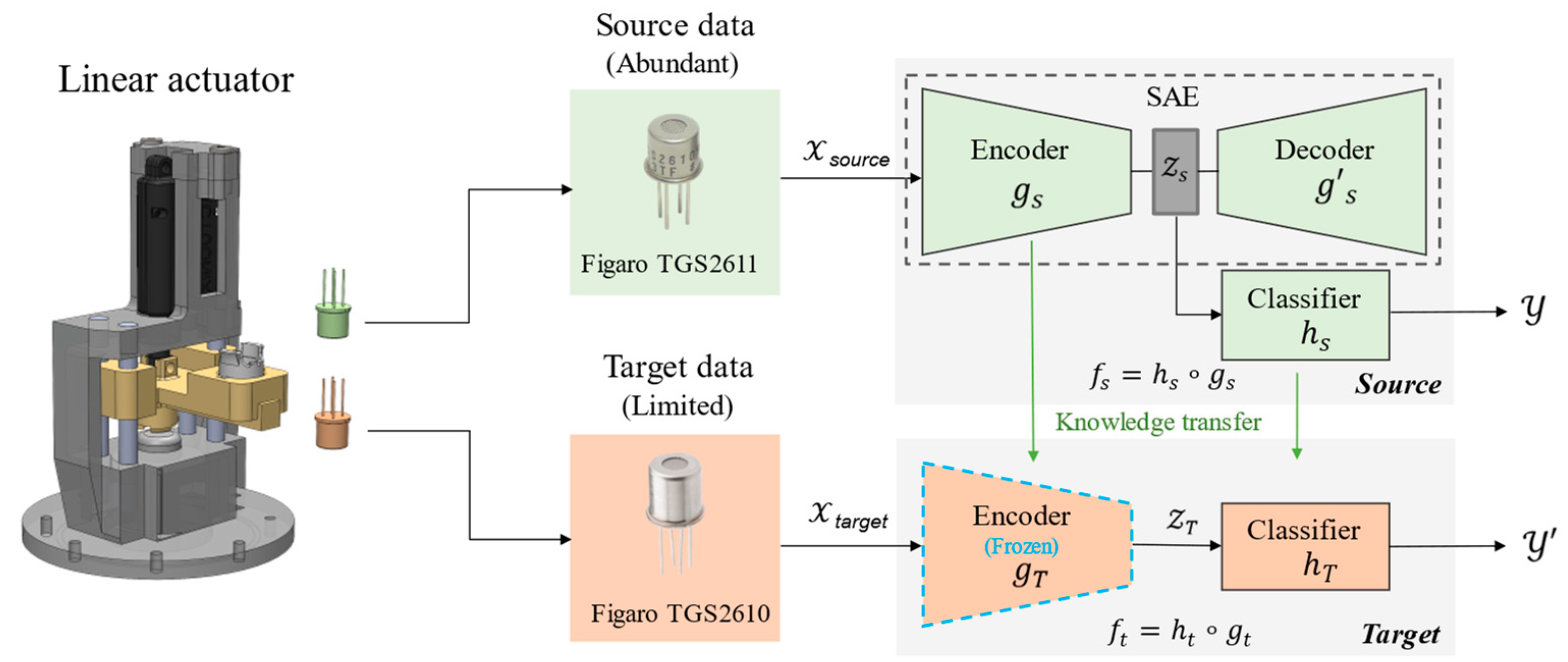
2. SAE-TL Framework
2.1. Sparse Autoencoder (SAE)
2.2. Transfer Learning
3. Experimental Verification
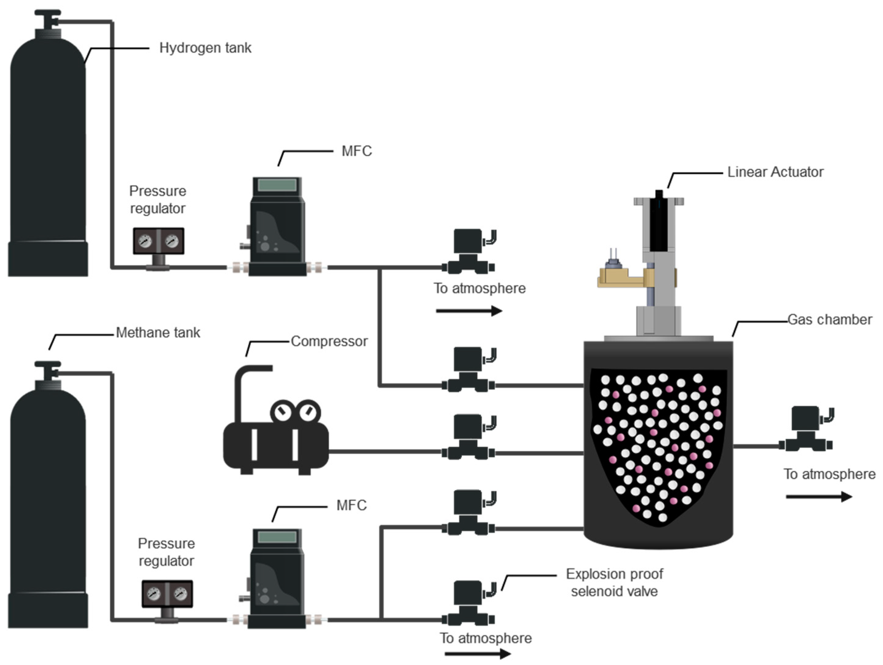
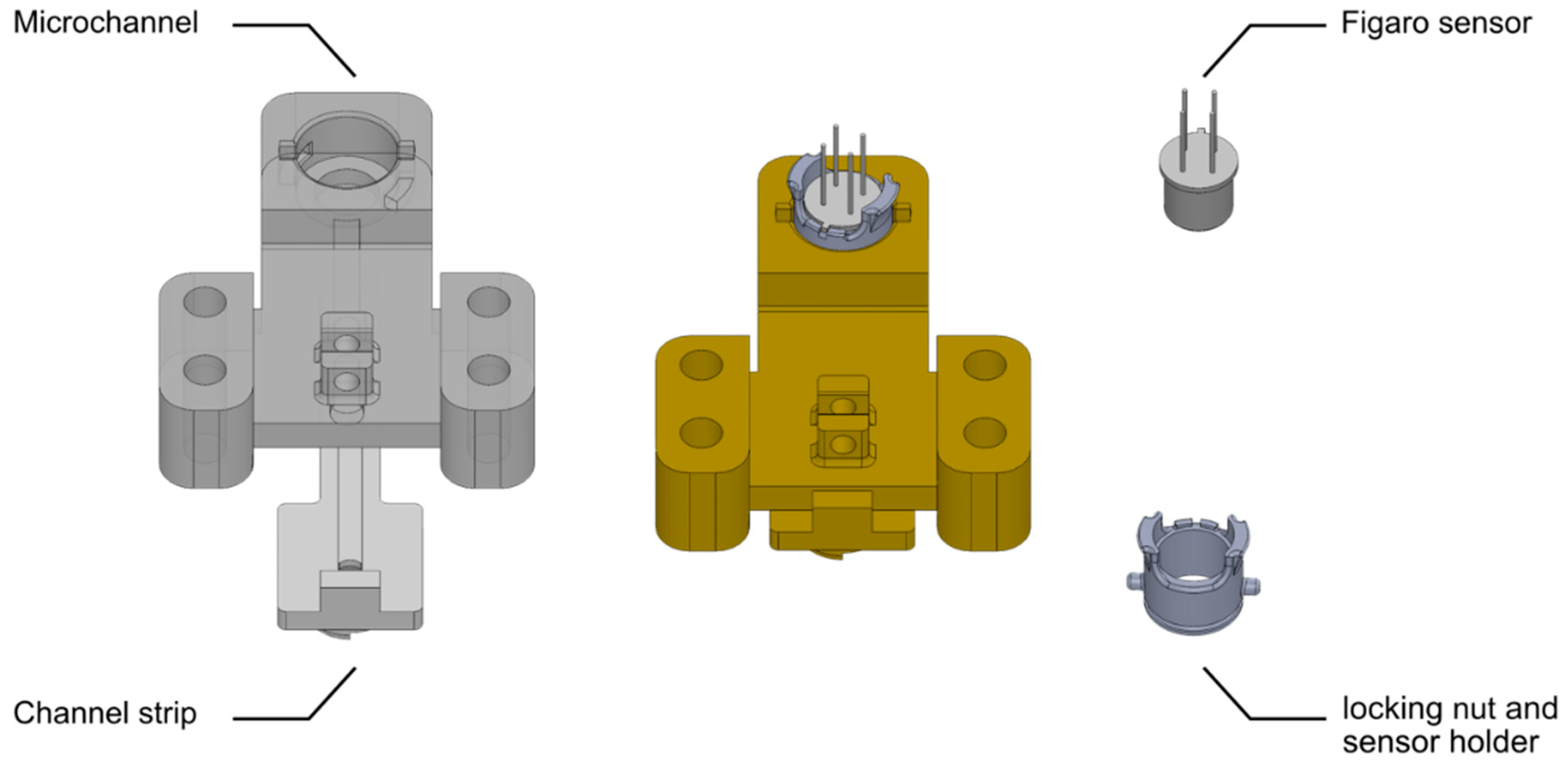
3.1. Case Study: Hydrogen Gas Detection Using a Microfluidic Detector
3.2. Sensor Characteristics
3.3. Gas Mixture
3.4. SAE-TL Experimental Design
4. Results and Discussion
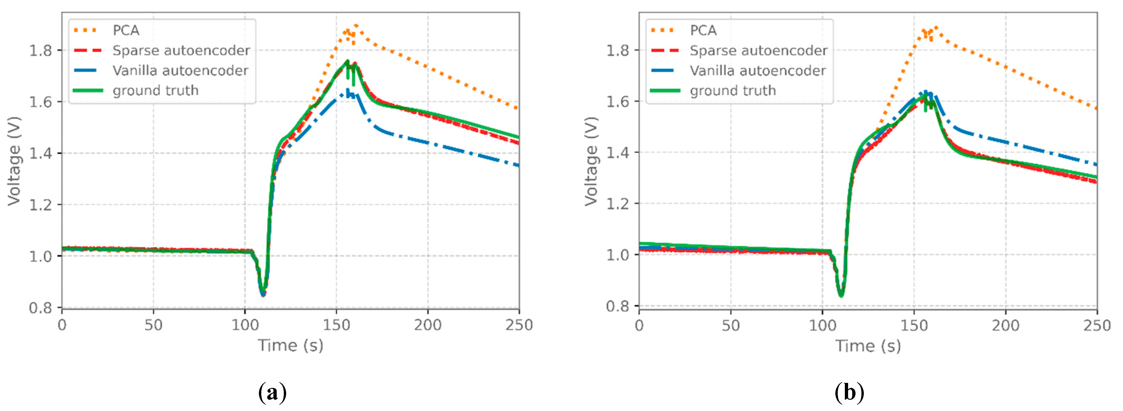
4.1. SAE Performance Evaluation
4.2. TL Performance Evaluation
5. Conclusions
Author Contributions
Funding
Institutional Review Board Statement
Informed Consent Statement
Conflicts of Interest
References
- Sagar, S.M.V.; Agarwal, A.K. Hydrogen-Enriched Compressed Natural Gas: An Alternate Fuel for IC Engines. In Advances in Internal Combustion Engine Research; Springer: Singapore, 2018; pp. 111–134. [Google Scholar]
- Melaina, M.W.; Antonia, O.; Penev, M. Blending Hydrogen into Natural Gas Pipeline Networks: A Review of Key Issues; NREL: Golden, CO, USA, 2013.
- Sparkman, O.D.; Penton, Z.; Kitson, F.G. Gas Chromatography and Mass Spectrometry: A Practical Guide; Elsevier Inc.: Amsterdam, The Netherlands, 2011. [Google Scholar]
- She, X.; Shen, Y.; Wang, J.; Jin, C. Pd films on soft substrates: A visual, high-contrast and low-cost optical hydrogen sensor. Light Sci. Appl. 2019, 8, 2047–7538. [Google Scholar] [CrossRef]
- Aray, A.; Ranjbar, M.; Shokoufi, N.; Morshedi, A. Plasmonic fiber optic hydrogen sensor using oxygen defects in nanostructured molybdenum trioxide film. Opt. Lett. 2019, 44, 4773. [Google Scholar] [CrossRef]
- Kalyakin, A.; Volkov, A.; Lyagaeva, J.; Medvedev, D.; Demin, A.; Tsiakaras, P. Combined amperometric and potentiometric hydrogen sensors based on BaCe0.7Zr0.1Y0.2O3-δ proton-conducting ceramic. Sens. Actuators B Chem. 2016, 231, 175–182. [Google Scholar] [CrossRef]
- Li, Y.; Li, X.; Tang, Z.; Wang, J.; Yu, J.; Tang, Z. Potentiometric hydrogen sensors based on yttria-stabilized zirconia electrolyte (YSZ) and CdWO4 interface. Sens. Actuators B Chem. 2016, 223, 365–371. [Google Scholar] [CrossRef]
- Lee, E.B.; Hwang, I.-S.; Cha, J.-H.; Lee, H.-J.; Lee, W.-B.; Pak, J.J.; Lee, J.-H.; Ju, B.-K. Micromachined catalytic combustible hydrogen gas sensor. Sens. Actuators B Chem. 2011, 153, 392–397. [Google Scholar] [CrossRef]
- Nishibori, M.; Shin, W.; Izu, N.; Itoh, T.; Matsubara, I.; Yasuda, S.; Ohtani, S. Robust hydrogen detection system with a thermoelectric hydrogen sensor for hydrogen station application. Int. J. Hydrog. Energy 2009, 34, 2834–2841. [Google Scholar] [CrossRef]
- Baek, D.H.; Kim, J. MoS2 gas sensor functionalized by Pd for the detection of hydrogen. Sens. Actuators B Chem. 2017, 250, 686–691. [Google Scholar] [CrossRef]
- Lu, C.T.; Lin, K.W.; Chen, H.I.; Chuang, H.M.; Chen, C.Y.; Liu, W.C. A new Pd-oxide-Al0.3Ga0.7As MOS hydrogen sensor. IEEE Electron. Device Lett. 2003, 24, 390–392. [Google Scholar] [CrossRef]
- Han, C.H.; Han, S.D.; Singh, I.; Toupance, T. Micro-bead of nano-crystalline F-doped SnO2 as a sensitive hydrogen gas sensor. Sens. Actuators B Chem. 2005, 109, 264–269. [Google Scholar] [CrossRef]
- Ippolito, S.J.; Kandasamy, S.; Kalantar-Zadeh, K.; Wlodarski, W. Hydrogen sensing characteristics of WO3 thin film conductometric sensors activated by Pt and Au catalysts. Sens. Actuators B Chem. 2005, 108, 154–158. [Google Scholar] [CrossRef]
- Dey, A. Semiconductor metal oxide gas sensors: A review. Mater. Sci. Eng. B Solid-State Mater. Adv. Technol. 2018, 229, 206–217. [Google Scholar] [CrossRef]
- Paknahad, M.; Bachhal, J.S.; Ahmadi, A.; Hoorfar, M. Characterization of channel coating and dimensions of microfluidic-based gas detectors. Sens. Actuators B Chem. 2017, 241, 55–64. [Google Scholar] [CrossRef]
- Yan, J.; Guo, X.; Duan, S.; Jia, P.; Wang, L.; Peng, C.; Zhang, S. Electronic nose feature extraction methods: A review. Sensors 2015, 15, 27804–27831. [Google Scholar]
- Hastie, T.; Tibshirani, R.; Friedman, J.; Franklin, J. The elements of statistical learning: Data mining, inference and prediction. Math. Intell. 2005, 27, 83–85. [Google Scholar]
- Goodfellow, I.; Bengio, Y.; Courville, A. Deep Learning; MIT Press: Cambridge, MA, USA, 2016. [Google Scholar]
- Cao, L.J.; Chua, K.S.; Chong, W.K.; Lee, H.P.; Gu, Q.M. A comparison of PCA, KPCA and ICA for dimensionality reduction in support vector machine. Neurocomputing 2003, 55, 321–336. [Google Scholar] [CrossRef]
- Yin, Y.; Tian, X. Classification of Chinese drinks by a gas sensors array and combination of the PCA with Wilks distribution. Sens. Actuators B Chem. 2007, 124, 393–397. [Google Scholar]
- Bengio, Y. Learning Deep Architectures for AI; Now Publishers Inc.: Boston, MA, USA, 2009. [Google Scholar]
- Baldi, P. Autoencoders, unsupervised learning, and deep architectures. Proc. ICML Workshop Unsupervised Transf. Learn. 2012, 27, 37–49. [Google Scholar]
- Zhao, W.; Meng, Q.-H.; Zeng, M.; Qi, P.-F. Stacked sparse auto-encoders (SSAE) based electronic nose for Chinese liquors classification. Sensors 2017, 17, 2855. [Google Scholar]
- Ma, D.; Gao, J.; Zhang, Z.; Zhao, H. Gas recognition method based on the deep learning model of sensor array response map. Sens. Actuators B Chem. 2021, 330, 129349. [Google Scholar]
- Pan, S.J.; Yang, Q. A Survey on Transfer Learning. IEEE Trans. Knowl. Data Eng. 2010, 22, 1345–1359. [Google Scholar] [CrossRef]
- Yan, K.; Zhang, D. Calibration transfer and drift compensation of e-noses via coupled task learning. Sens. Actuators B Chem. 2016, 225, 288–297. [Google Scholar]
- Yi, R.; Yan, J.; Shi, D.; Tian, Y.; Chen, F.; Wang, Z.; Duan, S. Improving the performance of drifted/shifted electronic nose systems by cross-domain transfer using common transfer samples. Sens. Actuators B Chem. 2021, 329, 129162. [Google Scholar]
- Barriault, M.; Alexander, I.; Tasnim, N.; O’Brien, A.; Najjaran, H.; Hoorfar, M. Classification and Regression of Binary Hydrocarbon Mixtures using Single Metal Oxide Semiconductor Sensor With Application to Natural Gas Detection. Sens. Actuators B Chem. 2021, 326, 129012. [Google Scholar] [CrossRef]
- Gamboa, J.C.R.; da Silva, A.J.; Araujo, I.C.S. Validation of the rapid detection approach for enhancing the electronic nose systems performance, using different deep learning models and support vector machines. Sens. Actuators B Chem. 2021, 327, 128921. [Google Scholar]
- Ramezankhani, M.; Crawford, B.; Narayan, A.; Voggenreiter, H.; Seethaler, R.; Milani, A.S. Making costly manufacturing smart with transfer learning under limited data: A case study on composites autoclave processing. J. Manuf. Syst. 2021, 59, 345–354. [Google Scholar] [CrossRef]
- Finn, C.; Abbeel, P.; Levine, S. Model-Agnostic Meta-Learning for Fast Adaptation of Deep Networks. In Proceedings of the International Conference on Machine Learning, Sydney, Australia, 6–11 August 2017; pp. 1126–1135. Available online: http://arxiv.org/abs/1703.03400 (accessed on 18 July 2017).
- Yosinski, J.; Clune, J.; Bengio, Y.; Lipson, H. How transferable are features in deep neural networks? Adv. Neural Inf. Process. Syst. 2014, 4, 3320–3328. [Google Scholar]
- Neyshabur, B.; Sedghi, H.; Zhang, C. What is being transferred in transfer learning? arXiv 2020, arXiv:2008.11687. [Google Scholar]
- Ramezankhani, M.; Narayan, A.; Seethaler, R.; Milani, A.S. An Active Transfer Learning (ATL) Framework for Smart Manufacturing with Limited Data: Case Study on Material Transfer in Composites Processing. In Proceedings of the 2021 4th IEEE International Conference on Industrial Cyber-Physical Systems (ICPS), Victoria, BC, Canada, 10–12 May 2021; pp. 277–282. [Google Scholar] [CrossRef]
- Hall, J.E.; Hooker, P.; Jeffrey, K.E. Gas detection of hydrogen/natural gas blends in the gas industry. Int. J. Hydrog. Energy 2020, 46, 12555–12565. [Google Scholar] [CrossRef]
- Montazeri, M.M.; De Vries, N.; Afantchao, A.; Mehrabi, P.; Kim, E.; O’Brien, A.; Najjaran, H.; Hoorfar, M.; Kadota, P. A sensor for nuisance sewer gas monitoring. In Proceedings of the IEEE Sensors, Glasgow, UK, 29 October–1 November 2017; Volume 2017, pp. 1–3. [Google Scholar] [CrossRef]
- Ahmadou, D.; Laref, R.; Losson, E.; Siadat, M. Reduction of drift impact in gas sensor response to improve quantitative odor analysis. In Proceedings of the IEEE International Conference on Industrial Technology (ICIT), Toronto, ON, Canada, 22–25 March 2017; pp. 928–933. [Google Scholar] [CrossRef]
- Paknahad, M.; Ahmadi, A.; Rousseau, J.; Nejad, H.R.; Hoorfar, M. On-Chip Electronic Nose For Wine Tasting: A Digital Microfluidic Approach. IEEE Sens. J. 2017, 17, 4322–4329. [Google Scholar] [CrossRef]
- Samarasekara, P. Hydrogen and methane gas sensors synthesis of multi-walled carbon nanotubes. Chin. J. Phys. 2009, 47, 361–369. [Google Scholar]
- Park, N.-H.; Akamatsu, T.; Itoh, T.; Izu, N.; Shin, W. Calorimetric thermoelectric gas sensor for the detection of hydrogen, methane and mixed gases. Sensors 2014, 14, 8350–8362. [Google Scholar]
- Brahim-Belhouari, S.; Bermak, A.; Shi, M.; Chan, P.C.H. Fast and robust gas identification system using an integrated gas sensor technology and Gaussian mixture models. IEEE Sens. J. 2005, 5, 1433–1444. [Google Scholar]
- Westerwaal, R.; Gersen, S.; Ngene, P.; Darmeveil, H.; Schreuders, H.; Middelkoop, J.; Dam, B. Fiber optic hydrogen sensor for a continuously monitoring of the partial hydrogen pressure in the natural gas grid. Sens. Actuators B Chem. 2014, 199, 127–132. [Google Scholar]
- Blokland, H.; Sweelssen, J.; Isaac, T.; Boersma, A. Detecting hydrogen concentrations during admixing hydrogen in natural gas grids. Int. J. Hydrog. Energy 2021, 46, 32318–32330. [Google Scholar]
- Ashkarran, A.A.; Olfatbakhsh, T.; Ramezankhani, M.; Crist, R.C.; Berrettini, W.H.; Milani, A.S.; Pakpour, S.; Mahmoudi, M. Evolving magnetically levitated plasma proteins detects opioid use disorder as a model disease. Adv. Healthc. Mater. 2020, 9, 1901608. [Google Scholar]
- Li, Q.; Gu, Y.; Wang, N.-F. Application of random forest classifier by means of a QCM-based e-nose in the identification of Chinese liquor flavors. IEEE Sens. J. 2017, 17, 1788–1794. [Google Scholar]
- Ke, G.; Meng, Q.; Finley, T.; Wang, T.; Chen, W.; Ma, W.; Ye, Q.; Liu, T.Y. Lightgbm: A highly efficient gradient boosting decision tree. Adv. Neural Inf. Process. Syst. 2017, 30, 3146–3154. [Google Scholar]
- Ramezankhani, M.; Crawford, B.; Khayyam, H.; Naebe, M.; Seethaler, R.; Milani, A.S. A multi-objective Gaussian process approach for optimization and prediction of carbonization process in carbon fiber production under uncertainty. Adv. Compos. Hybrid Mater. 2019, 2, 444–455. [Google Scholar] [CrossRef]
- Gal, Y.; Ghahramani, Z. Dropout as a bayesian approximation: Representing model uncertainty in deep learning. In Proceedings of the 33rd International Conference on Machine Learning, New York, NY, USA, 19–24 June 2016; pp. 1050–1059. [Google Scholar]


| Ref | Sensor Type | Limit of Detection | Power Consumption | Time from Collection to Results |
|---|---|---|---|---|
| [39] | Carbon nanotube/SiO2 | Not reported | Not reported | 1132 s |
| [40] | Calorimetric Pd/θ-Al2O3 | 200 ppm | 0.12 W | Not reported |
| [41] | Au/SnO2, Pt/Cu/SnO2 | 500 ppm | 200 mW | 180 s |
| [42] | Pd/Au optical sensor | 987 ppm | Not reported | 90 s |
| [43] | Semiconductor, Catalytic, electrochemical | 200 ppm | Not reported | 190–270 s |
| This Work | Semiconductor | 89 ppm | 200 mW | 150 s |
| Number of Hidden Layers | |||||
|---|---|---|---|---|---|
| 1 | 3 | 5 | 7 | 9 | |
| SAE | 0.00035 ± 0.00001 | 0.00031 ± 0.00002 | 0.00024 ± 0.00001 | 0.00034 ± 0.00002 | 0.00039 ± 0.0001 |
| AE | 0.0017 ± 0.00002 | 0.001 ± 0.00001 | 0.0007 ± 0.00001 | 0.008 ± 0.0001 | 0.0008 ± 0.0001 |
| Encoder | Regressor | MAE (ppm) | R-Squared |
|---|---|---|---|
| SAE-TL | MLP | 89.24 | 0.94 |
| AE-TL | MLP | 99.74 | 0.89 |
| PCA (Source) | XGBoost | 172.77 | 0.82 |
| RF | 206.53 | 0.67 | |
| SVM | 202.47 | 0.63 | |
| PCA (Source + Target) | XGBoost | 172.77 | 0.82 |
| RF | 176.82 | 0.73 | |
| SVM | 109.88 | 0.87 | |
| NN | 121.25 | 0.84 | |
Publisher’s Note: MDPI stays neutral with regard to jurisdictional claims in published maps and institutional affiliations. |
© 2022 by the authors. Licensee MDPI, Basel, Switzerland. This article is an open access article distributed under the terms and conditions of the Creative Commons Attribution (CC BY) license (https://creativecommons.org/licenses/by/4.0/).
Share and Cite
Mirzaei, H.; Ramezankhani, M.; Earl, E.; Tasnim, N.; Milani, A.S.; Hoorfar, M. Investigation of a Sparse Autoencoder-Based Feature Transfer Learning Framework for Hydrogen Monitoring Using Microfluidic Olfaction Detectors. Sensors 2022, 22, 7696. https://doi.org/10.3390/s22207696
Mirzaei H, Ramezankhani M, Earl E, Tasnim N, Milani AS, Hoorfar M. Investigation of a Sparse Autoencoder-Based Feature Transfer Learning Framework for Hydrogen Monitoring Using Microfluidic Olfaction Detectors. Sensors. 2022; 22(20):7696. https://doi.org/10.3390/s22207696
Chicago/Turabian StyleMirzaei, Hamed, Milad Ramezankhani, Emily Earl, Nishat Tasnim, Abbas S. Milani, and Mina Hoorfar. 2022. "Investigation of a Sparse Autoencoder-Based Feature Transfer Learning Framework for Hydrogen Monitoring Using Microfluidic Olfaction Detectors" Sensors 22, no. 20: 7696. https://doi.org/10.3390/s22207696
APA StyleMirzaei, H., Ramezankhani, M., Earl, E., Tasnim, N., Milani, A. S., & Hoorfar, M. (2022). Investigation of a Sparse Autoencoder-Based Feature Transfer Learning Framework for Hydrogen Monitoring Using Microfluidic Olfaction Detectors. Sensors, 22(20), 7696. https://doi.org/10.3390/s22207696