
An Ultra-Fast TSP on a CNT Heating Layer for Unsteady Temperature and Heat Flux Measurements in Subsonic Flows


Abstract
:1. Introduction
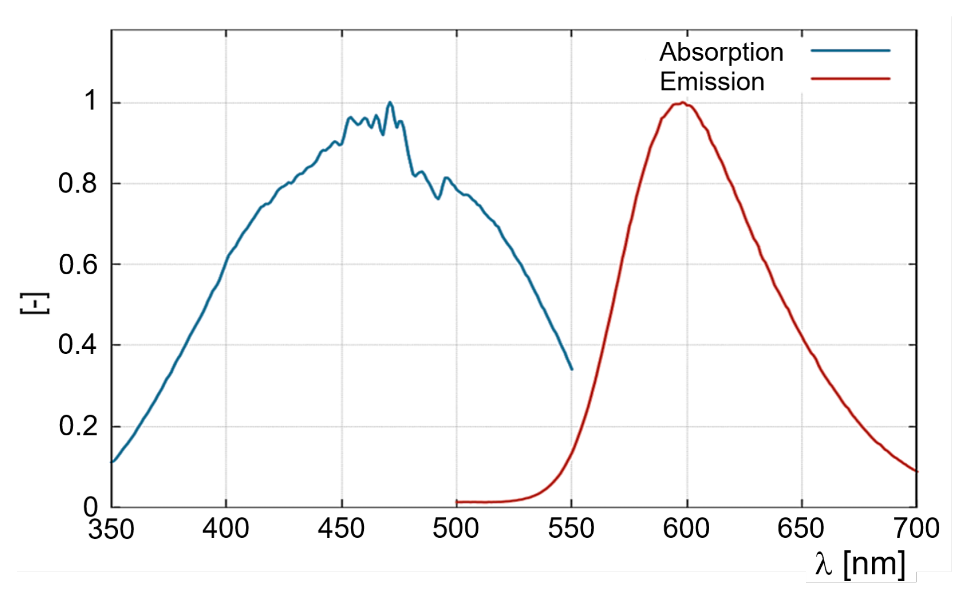
2. Modified Fast-Response Temperature Sensitive Paint
3. Test Environment and Methodology
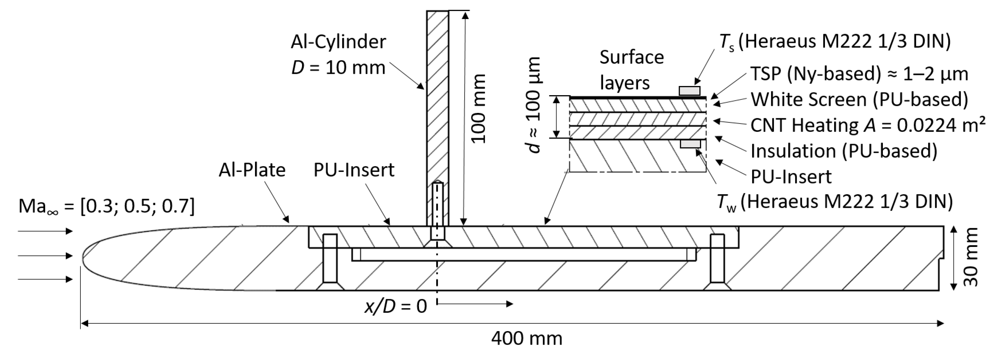
3.1. Experimental Setup
3.2. Methodology
3.2.1. Operating Conditions
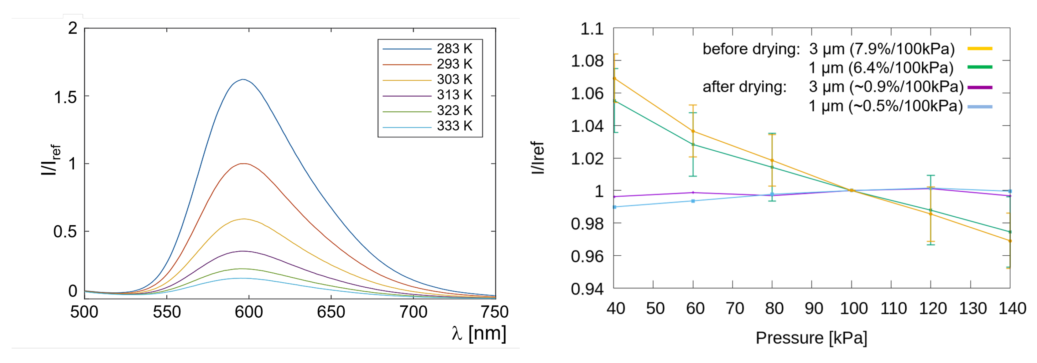
3.2.2. TSP Calibration
3.2.3. Image Acquisition and Data Reduction
3.2.4. Heat Transfer Coefficient
- An electric voltage setting was applied to the CNT layer which results in a heated surface. The model was allowed to stabilize its conditions which were monitored by the internal and external sensors and .
- The heat flux was calculated from the current and voltage given by the power supply according to .
- The surface temperature was measured with TSP and averaged at each set point.
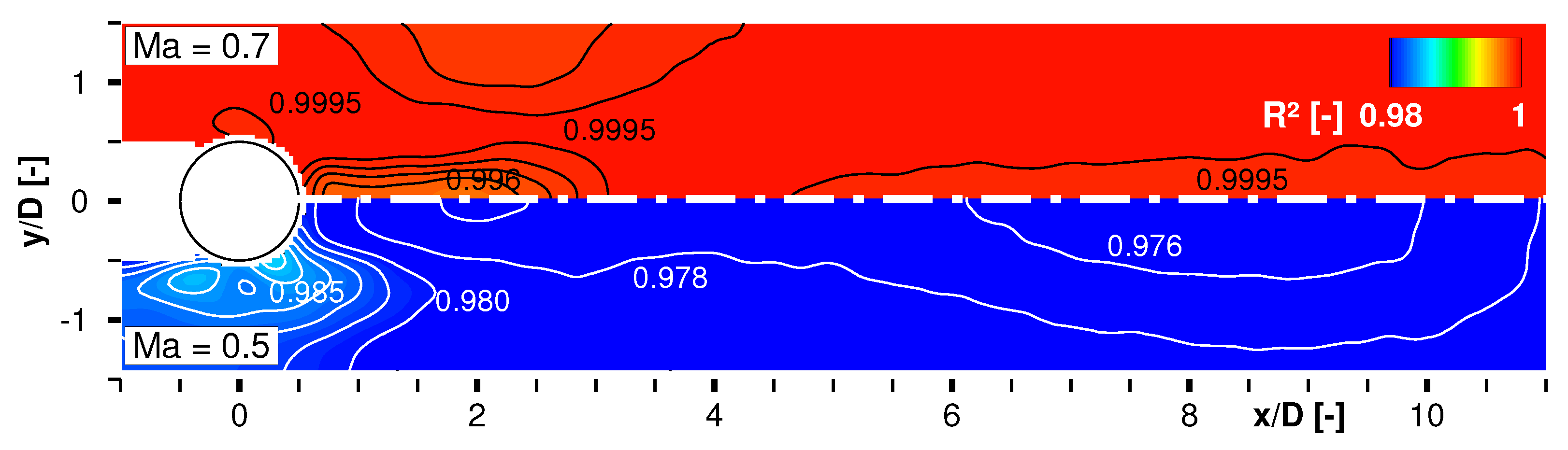
4. Results
5. Summary and Outlook
Author Contributions
Funding
Institutional Review Board Statement
Informed Consent Statement
Data Availability Statement
Acknowledgments
Conflicts of Interest
Abbreviations
| CNT | Carbon nanotubes |
| FFT | Fast Fourier transformation |
| FOV | Field of view |
| HGK | High-Speed Cascade Wind Tunnel of the Bundeswehr University Munich |
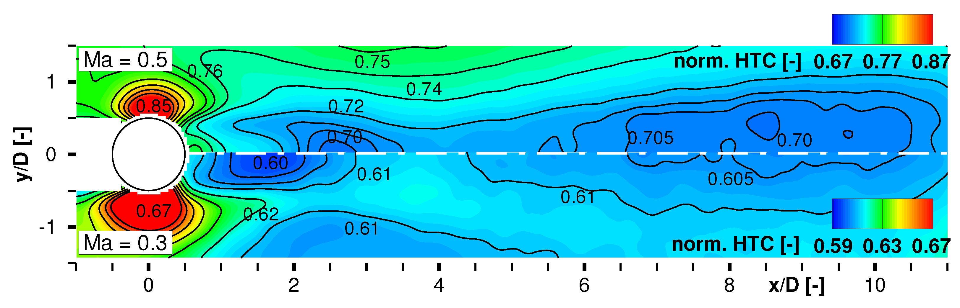
| HTC | Heat transfer coefficient, quasi-HTC = |
| LED | Light-emitting diode |
| Ny | Nylon |
| PA, PU | Poly-amide, poly-urethane |
| P-/TSP | Pressure-/Temperature-Sensitive Paint |
| Ru(phen) | Dichlorotris (1,10-phenanthroline) Ruthenium(II) hydrate 98% |
| RTD | Resistant temperature detector |
| SNR | Signal-to-noise ratio |
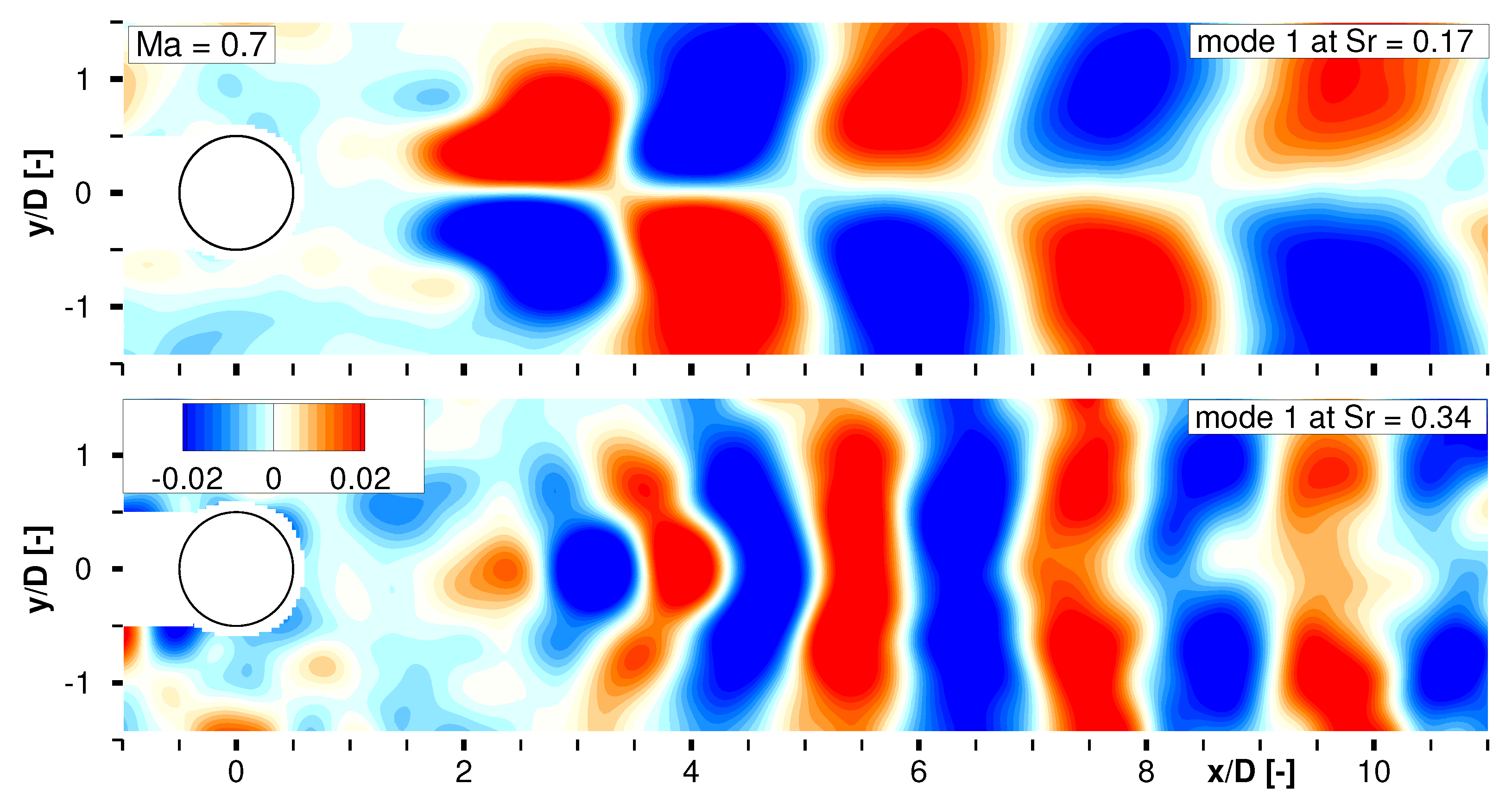
| SPOD | Spectral proper orthogonal decomposition (after [20]) |
Symbols
| Heat transfer coefficient [W/(mK)] | |
| Heated CNT surface area [m] | |
| d | Layer thickness [m] |
| D | Cylinder diameter [mm] |
| f | Frequency [Hz] |
| Heat capacity ratio [-] | |
| k | Thermal conductivity [W/(mK)] |
| Wavelength [nm] | |
| Inflow Mach number [-] | |
| Ambient pressure [kPa] | |
| Total pressure [kPa] | |
| Prandtl number [-] | |
| Dynamic pressure [kPa] | |
| Electrically generated heat flux [W/m] | |
| Conductive heat flux [W/m] | |
| Convective heat flux [W/m] | |
| Radiative heat flux [W/m] | |
| r | Recovery factor[-] |
| Determination coefficient of a (linear) fit [-] | |
| Reynolds number based on cylinder diameter D = 10 mm [-] | |
| Non-dimensional frequency; Strouhal number | |
| Camera integration time [s] | |
| Temperature fluctuation [K] | |
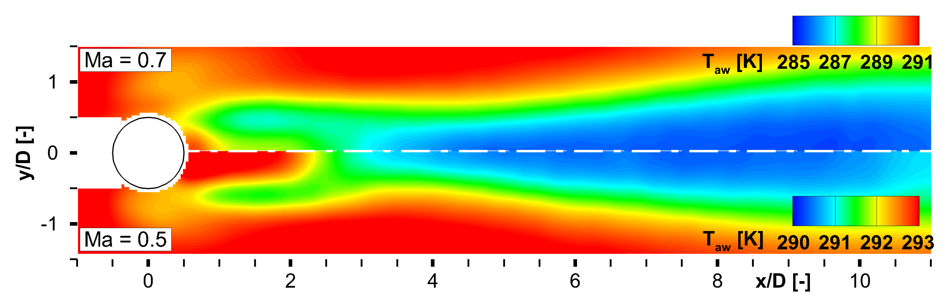
| Adiabatic wall temperature [K] | |
| Total temperature [K] | |
| Surface temperature field measured with TSP [K] | |
| Temperature at surface sensor [K] | |
| Temperature at wall sensor [K] | |
| u | Inflow velocity [m/s] |
| x; | Axial; normalized axial coordinate |
| y; | Span-wise; normalized span-wise coordinate |
References
- Liu, T.; Sullivan, J.P.; Asai, K.; Klein, C.; Egami, Y. Pressure and Temperature Sensitive Paints, 2nd ed.; Springer: Cham, Switzerland, 2021. [Google Scholar]
- Matsumura, S.; Berry, S.A.; Schneider, S.P. Flow Visualization Measurement Techniques for High-Speed Transition Research in the Boeing/AFOSR Mach-6 Quiet Tunnel. In Proceedings of the 39th AIAA/ASME Joint Propulsion Conference and Exhibit, Huntsville, AL, USA, 20–23 July 2003; AIAA Paper 2003-4583. [Google Scholar]
- Gregory, J.W.; Sakaue, H.; Liu, T.; Sullivan, J.P. Fast Pressure-Sensitive Paint for Flow and Acoustic Diagnostics. Annu. Rev. Fluid Mech. 2014, 46, 303–330. [Google Scholar] [CrossRef]
- Laurence, S.J.; Ozawa, H.; Lieber, D.; Martinez Schramm, J.; Hannemann, K. Investigation of unsteady/quasi-steady scramjet behavior using high-speed visualization techniques. In Proceedings of the 18th AIAA International Space Planes and Hypersonic Systems and Technologies Conference, Tours, France, 24–28 September 2012. [Google Scholar]
- Martinez Schramm, J.; Hannemann, K.; Ozawa, H.; Beck, W.; Klein, C. Development of Temperature Sensitive Paints in the High Enthalpy Shock Tunnel Göttingen, HEG. In Proceedings of the 8th European Symposium on Aerothermodynamics for Space Vehicles, Lisbon, Portugal, 2–6 March 2015. [Google Scholar]
- Ozawa, H. Experimental study of unsteady aerothermodynamic phenomena on shock-tube wall using fast-response temperature-sensitive-paints. Phys. Fluids 2016, 28, 046103. [Google Scholar] [CrossRef]
- Martinez Schramm, J.; Schmidt, L. Internal application of ultra-fast temperature sensitive paint to hydrogen combustion flow. In New Results in Numerical and Experimental Fluid Mechanics XIII; Dillmann, A., Heller, G., Krämer, E., Wagner, C., Tropea, C., Jakirlić, S., Eds.; Springer: Cham, Switzerland, 2021; pp. 121–131. [Google Scholar]
- Ozawa, H.; Laurence, S. Experimental investigation of the shock-induced flow over a wall-mounted cylinder. J. Fluid Mech. 2018, 849, 1009–1042. [Google Scholar] [CrossRef]
- Sharma, A.; Katiyar, M.; Deepak; Shukla, S.K.; Seki, S. Effect of ambient, excitation intensity and wavelength, and chemical structure on photodegradation in polysilanes. J. Appl. Phys. 2007, 102, 104902. [Google Scholar] [CrossRef]
- Klein, C.; Henne, U.; Sachs, W.; Beifuß, U.; Ondrus, V.; Bruse, M.; Lesjak, R.; Löhr, M. Application of Carbon Nanotubes (CNT) and Temperature-Sensitive Paint (TSP) for the Detection of Boundary Layer Transition. In Proceedings of the 52nd AIAA Aerospace Sciences Meeting (AIAA SciTech 2014), National Harbor, MD, USA, 13–17 January 2014. [Google Scholar]
- Klein, C.; Henne, U.; Yorita, D.; Beifuß, U.; Ondrus, V.; Hensch, A.-K.; Longo, R.; Hauser, M.; Guntermann, P.; Quest, J. Application of Carbon Nanotubes and Temperature-Sensitive Paint for the Detection of Boundary Layer Transition under Cryogenic Conditions. In Proceedings of the 55th AIAA Aerospace Sciences Meeting (AIAA SciTech 2017), Grapevine, TX, USA, 9–13 January 2017. [Google Scholar]
- Martinez Schramm, J.; Hilfer, M. Time response calibration of ultra-fast temperature sensitive paints for the application in high temperature hypersonic flows. In New Results in Numerical and Experimental Fluid Mechanics XII; Dillmann, A., Heller, G., Krämer, E., Wagner, C., Tropea, C., Jakirlić, S., Eds.; Springer: Cham, Switzerland, 2020; pp. 143–152. [Google Scholar]
- Miozzi, M.; Di Felice, F.; Klein, C.; Costantini, M. Taylor hypothesis applied to direct measurement of skin friction using data from Temperature Sensitive Paint. Exp. Therm. Fluid Sci. 2020, 110, 109913. [Google Scholar] [CrossRef]
- Schlichting, H.; Gersten, K. Grenzschicht-Theorie; 10. Auflage; Springer: Berlin/Heidelberg, Germany, 2006; pp. 232–234. [Google Scholar]
- Tropea, C.; Yarin, L.A.; Foss, J.F. Handbook of Experimental Fluid Mechanics; Springer: Berlin/Heidelberg, Germany, 2007; Chapter 7.4; pp. 543–547. [Google Scholar]
- Schmidt, L. Application of Temperature Sensitive Paint to Determine the Heat Flux in a Hypersonic Hydrogen Combustion FLow. Bachelor’s Thesis, DLR, Göttingen, Germany, 2021. [Google Scholar]
- Dimond, B.D. (DLR, Göttingen, Germany); Hilfer, M. (DLR, Göttingen, Germany). Evaluation of Pressure Sensitivity of UHS-TSP. Internal communication, 2021.
- Niehuis, R.; Bitter, M. The High-Speed Cascade Wind Tunnel at the Bundeswehr University Munich after a Major Revision and Upgrade. Int. J. Turbomach. Propuls. Power 2021, 6, 41. [Google Scholar] [CrossRef]
- Zhang, C.; Moreau, S.; Sanjosé, M. Turbulent flow and noise sources on a circular cylinder in the critical regime. AIP Adv. 2019, 9, 085009. [Google Scholar] [CrossRef] [Green Version]
- Towne, A.; Schmidt, O.T.; Colonius, T. Spectral proper orthogonal decomposition and its relationship to dynamic mode decomposition and resolvent analysis. J. Fluid Mech. 2018, 847, 821–867. [Google Scholar] [CrossRef] [Green Version]
- Gomes, R.A.; Niehuis, R. Film Cooling Effectiveness Measurements on Highly Loaded Blades with Flow Separation. In Proceedings of the 8th European Conference on Turbomachinery (ETC), Graz, Austria, 23–27 March 2009. [Google Scholar]
- Liu, T.; Cai, Z.; Lai, J.; Rubal, J.; Sullivan, J.P. Analytical method for determining heat flux from temperature-sensitive-paint measurements in hypersonic tunnels. J. Thermophys. Heat Transf. 2010, 24, 85–94. [Google Scholar] [CrossRef]
- Aberle, S.; Bitter, M.; Hoefler, F.; Benignos, J.C.; Niehuis, R. Implementation of an In-Situ Infrared Calibration Method for Precise Heat Transfer Measurements on a Linear Cascade. J. Turbomach. 2019, 141, 021004. [Google Scholar] [CrossRef] [Green Version]
- Estorf, M. Image based heating rate calculation from thermographic data considering lateral heat conduction. Int. J. Heat Mass Transf. 2006, 49, 2545–2556. [Google Scholar] [CrossRef]
- Liu, T.; Campbell, B.; Sullivan, J. Heat Transfer Measurement on a Waverider at Mach 10 Using Fluorescent Paint. J. Thermophys. Heat Transf. 1995, 9, 605–611. [Google Scholar] [CrossRef]
- Chen, L.; Kawase, C.; Nonamura, T.; Asai, K. Dynamic surface heat transfer and re-attachment flow measurement using luminescent molecular sensors. Int. J. Heat Mass Transf. 2020, 155, 119684. [Google Scholar] [CrossRef]
- Lehmkuhl, O.; Rodríguez, I.; Borrell, R.; Oliva, A. Low-frequency unsteadiness in the vortex formation region of a circular cylinder. Phys. Fluids 2013, 25, 085109. [Google Scholar] [CrossRef] [Green Version]
- Bitter, M.; Stotz, S.; Niehuis, R. On High-Resolution Pressure Amplitude and Phase Measurements Comparing Fast-Response Pressure Transducers and Unsteady Pressure-Sensitive Paint. J. Turbomach. 2021, 143, 031012. [Google Scholar] [CrossRef]


| [kPa] | [kPa] | [kPa] | [m/s] | [K] | [K] | [Hz] | ||
|---|---|---|---|---|---|---|---|---|
| 0.3 | 95k | 13.8 | 0.89 | 14.7 | 102.1 | 293.15 | 292.7 | 1850 |
| 0.5 | 165k | 13.8 | 2.57 | 16.4 | 167.4 | 293.15 | 291.9 | 2760 |
| 0.7 | 245k | 13.8 | 5.35 | 19.1 | 229.5 | 293.15 | 290.8 | 4320 |
| FOV | Frame Rate [Hz] | [s] | [nm] | [nm] | [s] |
|---|---|---|---|---|---|
| 40,000 | 1 | 570 LP |
| U [V] | I [A] | [W/m] | [K] | [K] | |
|---|---|---|---|---|---|
| 0.3 | |||||
| 0.5 | |||||
| 0.7 |
Publisher’s Note: MDPI stays neutral with regard to jurisdictional claims in published maps and institutional affiliations. |
© 2022 by the authors. Licensee MDPI, Basel, Switzerland. This article is an open access article distributed under the terms and conditions of the Creative Commons Attribution (CC BY) license (https://creativecommons.org/licenses/by/4.0/).
Share and Cite
Bitter, M.; Hilfer, M.; Schubert, T.; Klein, C.; Niehuis, R. An Ultra-Fast TSP on a CNT Heating Layer for Unsteady Temperature and Heat Flux Measurements in Subsonic Flows. Sensors 2022, 22, 657. https://doi.org/10.3390/s22020657
Bitter M, Hilfer M, Schubert T, Klein C, Niehuis R. An Ultra-Fast TSP on a CNT Heating Layer for Unsteady Temperature and Heat Flux Measurements in Subsonic Flows. Sensors. 2022; 22(2):657. https://doi.org/10.3390/s22020657
Chicago/Turabian StyleBitter, Martin, Michael Hilfer, Tobias Schubert, Christian Klein, and Reinhard Niehuis. 2022. "An Ultra-Fast TSP on a CNT Heating Layer for Unsteady Temperature and Heat Flux Measurements in Subsonic Flows" Sensors 22, no. 2: 657. https://doi.org/10.3390/s22020657
APA StyleBitter, M., Hilfer, M., Schubert, T., Klein, C., & Niehuis, R. (2022). An Ultra-Fast TSP on a CNT Heating Layer for Unsteady Temperature and Heat Flux Measurements in Subsonic Flows. Sensors, 22(2), 657. https://doi.org/10.3390/s22020657