
Interactive Deep Learning for Shelf Life Prediction of Muskmelons Based on an Active Learning Approach


Abstract
:1. Introduction
- guidance and sample efficient improvement of the DL algorithm through a human-in-the-loop setting,
- potential reduction of the required samples for training DL algorithm and
- introduction of k-DPP as a diverse sampling method with improved capture of the underlying data distribution compared to uncertainty-related metrics.
2. Materials and Methods
2.1. Data Collection
2.2. Experimental Design
2.3. Related Fields of Research
2.4. Dataset
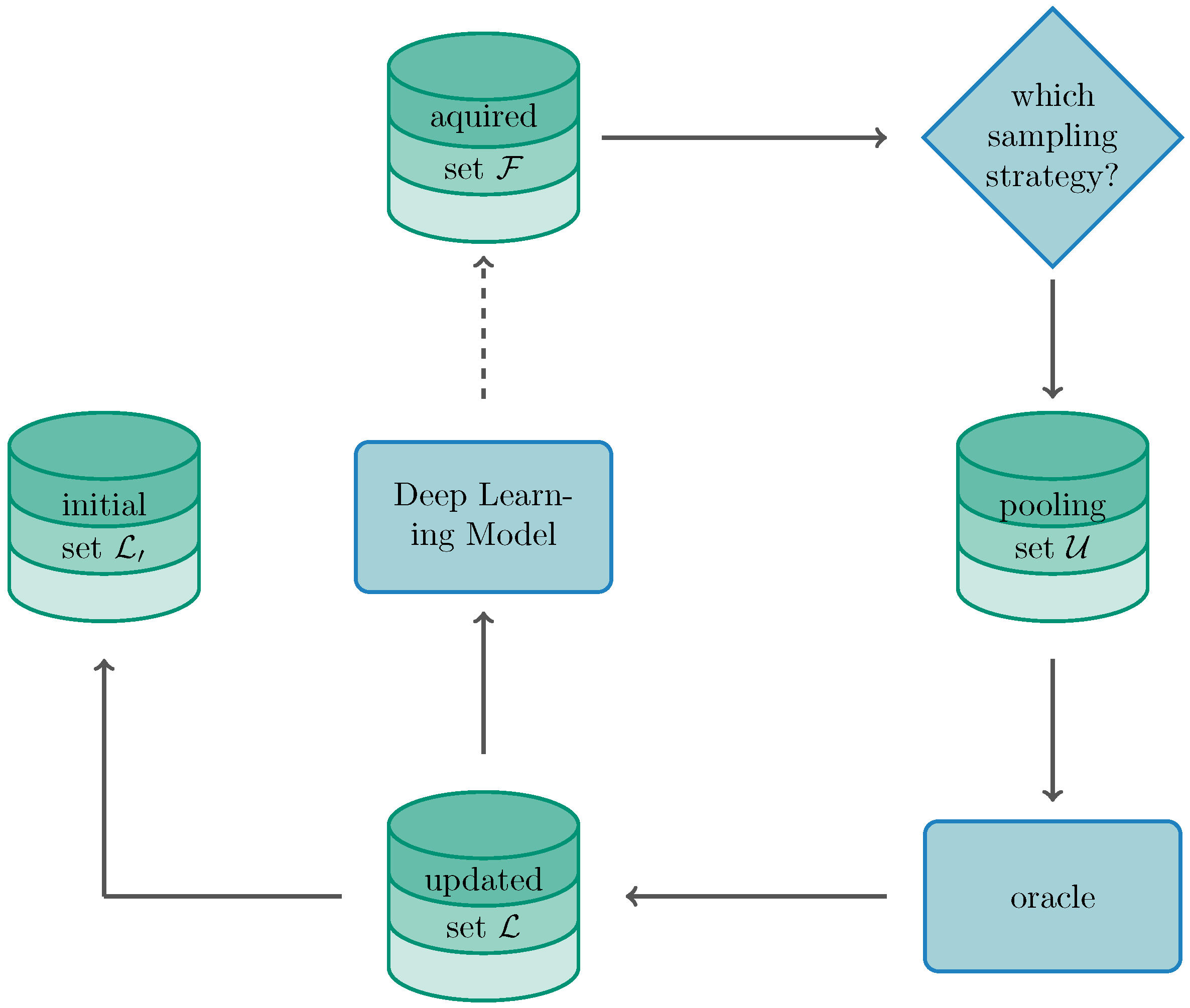
2.5. Active Learning Framework
2.6. Choice of Acquisition Function
- Random acquisition represents the baseline where instances are sampled stochastically without the heuristic calculation of a metric.
- Least Confidence samples the instances where the algorithm is least confident about the label and is calculated bywith posterior probability .
- Margin sampling calculates the margin between the most probable and second most probable classes represented by and :
- Maximum entropy samples instances yielding the maximum entropy by determining
- Ratio of confidence sampling is very closely related to margin sampling where the two scores with the highest probable classes are determined as a ratio instead of the difference.
- Bayesian Active Learning of Disagreement (BALD): The goal of BALD is to maximise the mutual information between the prediction and model posterior such that, under the prerequisite of being Bayesian, BALD can be stated aswith representing the entropy. Instances leading to a maximal score relate to points on which the algorithm is uncertain on average and for with the model parameters are referenced with a high disagreeing prediction [61,62].
- -Determinental Point Processes (-DPP): As an diversity-based approach, k-DPP takes an exploratory approach by sampling based on the DPP conditioned on the modelled set being of cardinality k [63] (We like to note that we prefer the use of k-DPP over traditional DPP due to the introduced bias into the modelling of the content. Parameter k allows to take a direct influence on the diversity by taking into regard the repulsiveness of the drawn samples—or in other words—the magnitude of the negative correlation between samples).
3. Results
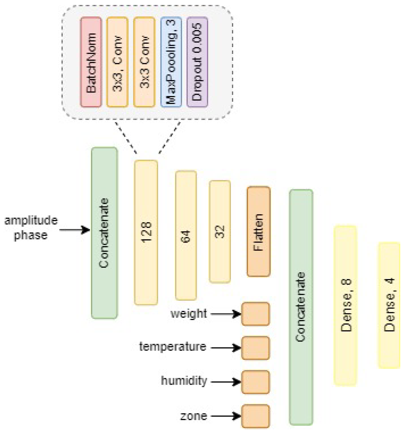
3.1. Model Training
3.2. Training Setting for Active Learning
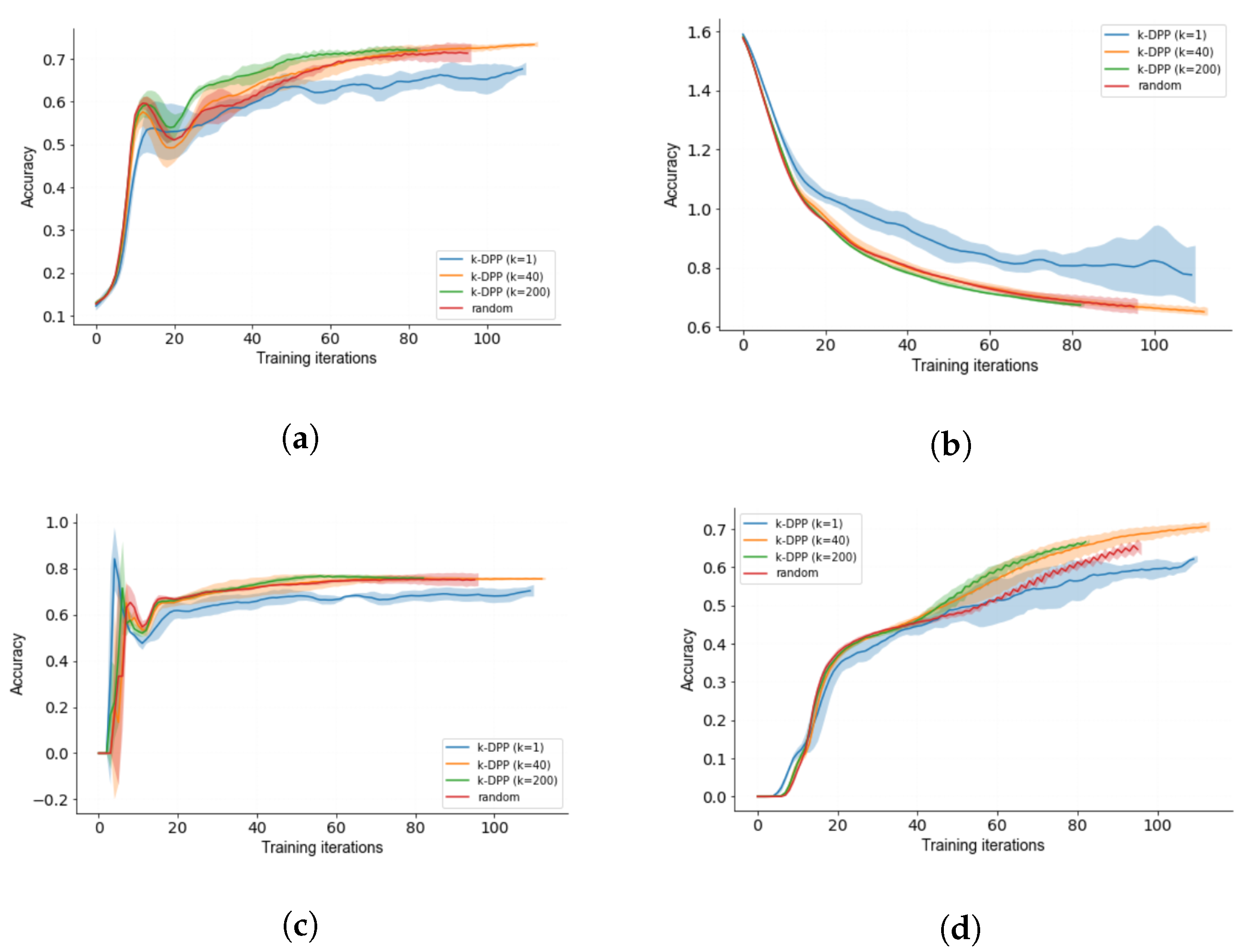
3.3. Diverse k-DPP Sampling
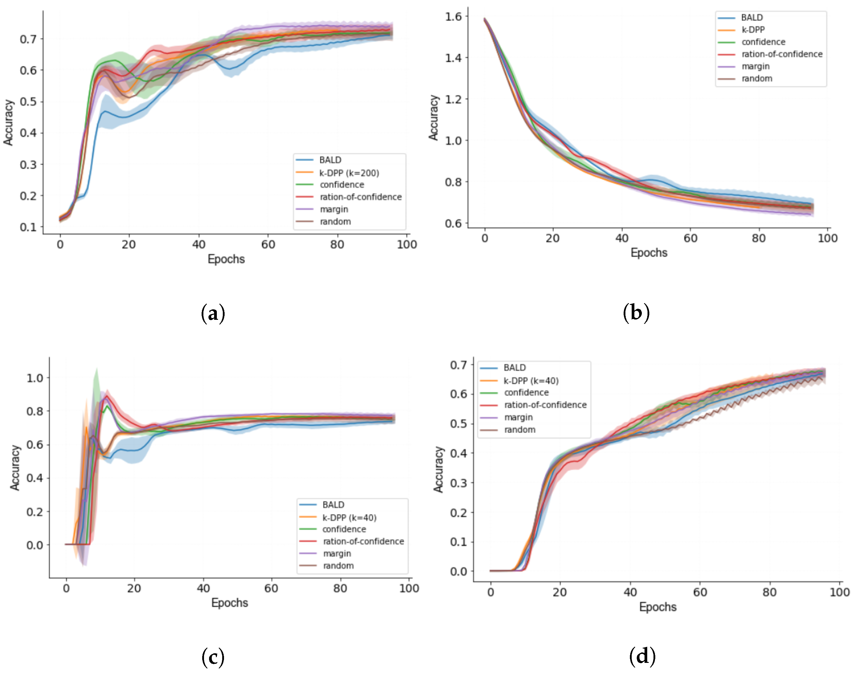
3.4. Human-in-the-Loop Performance
4. Discussion
5. Conclusions
Author Contributions
Funding
Institutional Review Board Statement
Informed Consent Statement
Data Availability Statement
Acknowledgments
Conflicts of Interest
Abbreviations
| AL | active learning |
| ART | Acoustic Resonance Testing |
| CNN | Convolutional Neural Network |
| DL | Deep Learning |
| DPP | Determinental Point Process |
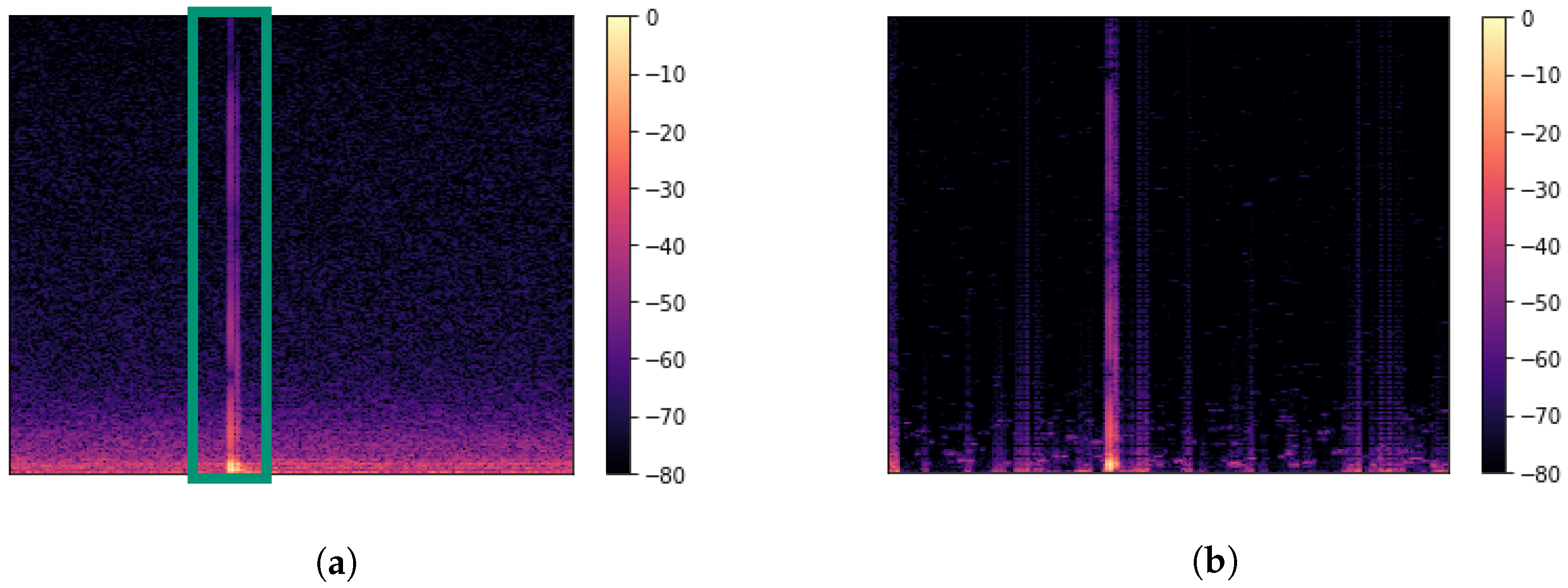
| SCNR | Single Channel Noise Reduction |
Appendix A
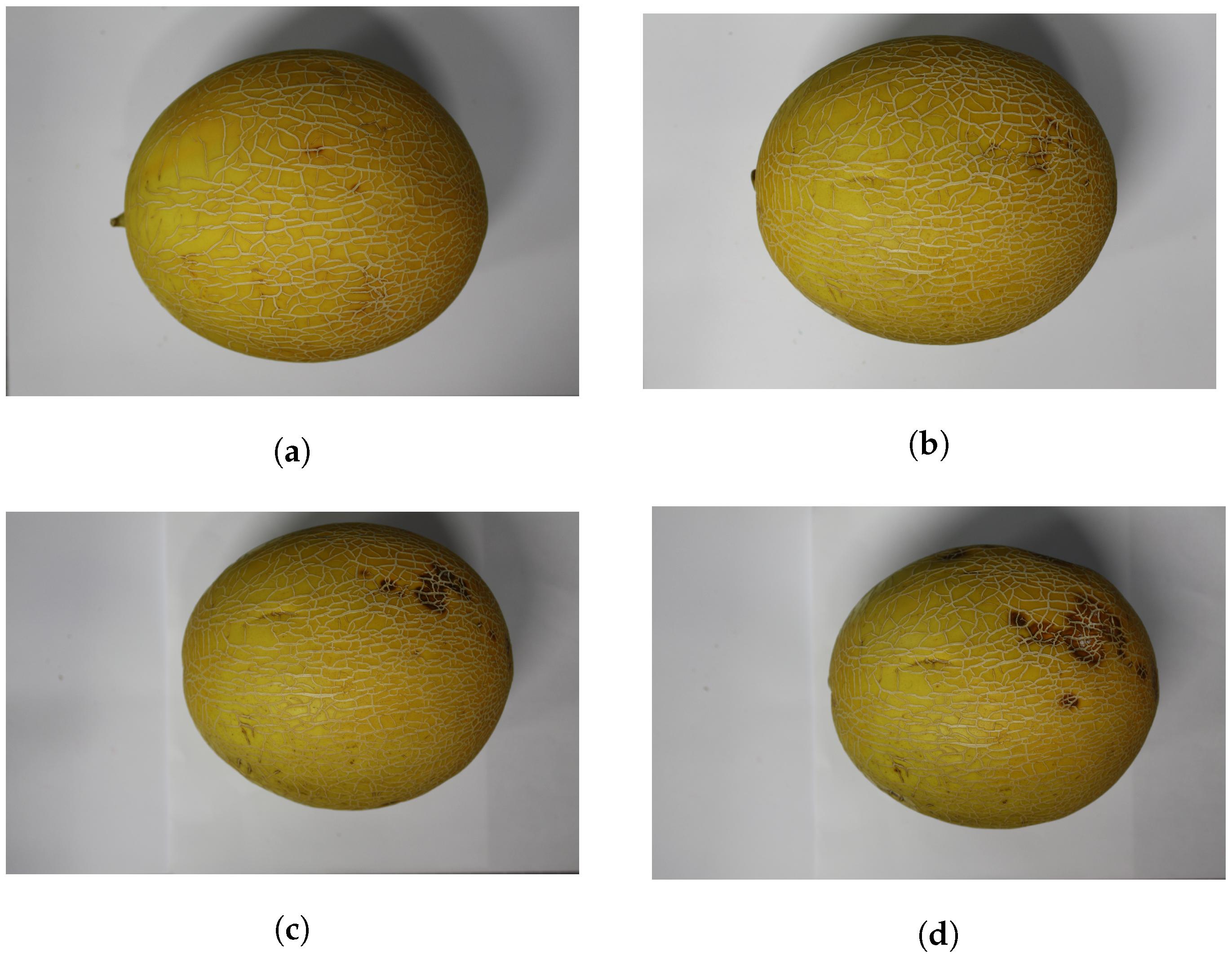
Appendix A.1. Images Galia Melon

Appendix A.2. Overview of Preselected Parameters

| Objective | Parameters | Value |
|---|---|---|
| weight span [g] | 837.2–1555.3 | |
| difference of the room temperature [°C] | 18.4–22.9 | |
| Dataset | difference room humidity [%] | 20.77–49.37 |
| measurements on shelf life s | {0, 7, 10, 15, 17, 62} | |
| Augmenation types | horizontal flipping, vertical flipping | |
| Preprocessing | Gain filter parameter | 9 |
| Gain filter parameter | 45 | |
| batch size | 64 | |
| learning rate | 0.005; exponential decay | |
| optimisation algorithm | SGD | |
| Hyperparameters | momentum | 0.9 |
| nestorov | activated | |
| clipping norm | 1.0 | |
| gradient clipping | 0.5 | |
| initial set | 30 | |
| Active Learning | initial set | 50 |
| k in k-DPP | {1, 40, 200} |
References
- Abasi, S.; Minaei, S.; Jamshidi, B.; Fathi, D. Dedicated non-destructive devices for food quality measurement: A review. Trends Food Sci. Technol. 2018, 78, 197–205. [Google Scholar] [CrossRef]
- Hussain, A.; Pu, H.; Sun, D.W. Innovative nondestructive imaging techniques for ripening and maturity of fruits—A review of recent applications. Trends Food Sci. Technol. 2018, 72, 144–152. [Google Scholar] [CrossRef]
- Mohd Ali, M.; Hashim, N.; Bejo, S.K.; Shamsudin, R. Rapid and nondestructive techniques for internal and external quality evaluation of watermelons: A review. Sci. Hortic. 2017, 225, 689–699. [Google Scholar] [CrossRef]
- Arendse, E.; Fawole, O.A.; Magwaza, L.S.; Opara, U.L. Non-destructive prediction of internal and external quality attributes of fruit with thick rind: A review. J. Food Eng. 2018, 217, 11–23. [Google Scholar] [CrossRef]
- Paul, V.; Pandey, R.; Srivastava, G.C. The fading distinctions between classical patterns of ripening in climacteric and non-climacteric fruit and the ubiquity of ethylene-An overview. J. Food Sci. Technol. 2012, 49, 1–21. [Google Scholar] [CrossRef] [Green Version]
- Arakeri, M.; Lakshmana. Computer Vision Based Fruit Grading System for Quality Evaluation of Tomato in Agriculture industry. Procedia Comput. Sci. 2016, 79, 426–433. [Google Scholar] [CrossRef] [Green Version]
- Brosnan, T.; Sun, D.W. Improving quality inspection of food products by computer vision—A review. J. Food Eng. 2004, 61, 3–16. [Google Scholar] [CrossRef]
- Bhargava, A.; Bansal, A. Fruits and vegetables quality evaluation using computer vision: A review. J. King Saud Univ. Comput. Inf. Sci. 2021, 33, 243–257. [Google Scholar] [CrossRef]
- Moallem, P.; Serajoddin, A.; Pourghassem, H. Computer vision-based apple grading for golden delicious apples based on surface features. Inf. Process. Agric. 2017, 4, 33–40. [Google Scholar] [CrossRef] [Green Version]
- Mohammadi, V.; Kheiralipour, K.; Ghasemi-Varnamkhasti, M. Detecting maturity of persimmon fruit based on image processing technique. Sci. Hortic. 2015, 184, 123–128. [Google Scholar] [CrossRef]
- Kotwaliwale, N.; Singh, K.; Kalne, A.; Jha, S.N.; Seth, N.; Kar, A. X-ray imaging methods for internal quality evaluation of agricultural produce. J. Food Sci. Technol. 2014, 51, 1–15. [Google Scholar] [CrossRef] [PubMed] [Green Version]
- Yang, L.; Yang, F.; Noguchi, N. Apple Internal Quality Classification Using X-ray and SVM. IFAC Proc. Vol. 2011, 44, 14145–14150. [Google Scholar] [CrossRef] [Green Version]
- Brezmes, J.; Fructuoso, M.; Llobet, E.; Vilanova, X.; Recasens, I.; Orts, J.; Saiz, G.; Correig, X. Evaluation of an electronic nose to assess fruit ripeness. IEEE Sens. J. 2005, 5, 97–108. [Google Scholar] [CrossRef] [Green Version]
- Gómez, A.H.; Hu, G.; Wang, J.; Pereira, A.G. Evaluation of tomato maturity by electronic nose. Comput. Electron. Agric. 2006, 54, 44–52. [Google Scholar] [CrossRef]
- Oh, S.H.; Lim, B.S.; Hong, S.J.; Lee, S.K. Aroma volatile changes of netted muskmelon (Cucumis melo L.) fruit during developmental stages. Hortic. Environ. Biotechnol. 2011, 52, 590–595. [Google Scholar] [CrossRef]
- Bureau, S.; Ruiz, D.; Reich, M.; Gouble, B.; Bertrand, D.; Audergon, J.M.; Renard, C.M. Rapid and non-destructive analysis of apricot fruit quality using FT-near-infrared spectroscopy. Food Chem. 2009, 113, 1323–1328. [Google Scholar] [CrossRef]
- Wang, H.; Peng, J.; Xie, C.; Bao, Y.; He, Y. Fruit quality evaluation using spectroscopy technology: A review. Sensors 2015, 15, 11889–11927. [Google Scholar] [CrossRef] [Green Version]
- Camps, C.; Christen, D. Non-destructive assessment of apricot fruit quality by portable visible-near infrared spectroscopy. LWT Food Sci. Technol. 2009, 42, 1125–1131. [Google Scholar] [CrossRef]
- Nicolaï, B.M.; Beullens, K.; Bobelyn, E.; Peirs, A.; Saeys, W.; Theron, K.I.; Lammertyn, J. Nondestructive measurement of fruit and vegetable quality by means of NIR spectroscopy: A review. Postharvest Biol. Technol. 2007, 46, 99–118. [Google Scholar] [CrossRef]
- Zhang, W.; Lv, Z.; Xiong, S. Nondestructive quality evaluation of agro-products using acoustic vibration methods-A review. Crit. Rev. Food Sci. Nutr. 2018, 58, 2386–2397. [Google Scholar] [CrossRef]
- Taniwaki, M.; Hanada, T.; Sakurai, N. Postharvest quality evaluation of “Fuyu” and “Taishuu” persimmons using a nondestructive vibrational method and an acoustic vibration technique. Postharvest Biol. Technol. 2009, 51, 80–85. [Google Scholar] [CrossRef]
- Primo-Martín, C.; Sözer, N.; Hamer, R.J.; van Vliet, T. Effect of water activity on fracture and acoustic characteristics of a crust model. J. Food Eng. 2009, 90, 277–284. [Google Scholar] [CrossRef]
- Arimi, J.M.; Duggan, E.; O’Sullivan, M.; Lyng, J.G.; O’Riordan, E.D. Effect of water activity on the crispiness of a biscuit (Crackerbread): Mechanical and acoustic evaluation. Food Res. Int. 2010, 43, 1650–1655. [Google Scholar] [CrossRef]
- Maruyama, T.T.; Arce, A.I.C.; Ribeiro, L.P.; Costa, E.J.X. Time–frequency analysis of acoustic noise produced by breaking of crisp biscuits. J. Food Eng. 2008, 86, 100–104. [Google Scholar] [CrossRef]
- Piazza, L.; Gigli, J.; Ballabio, D. On the application of chemometrics for the study of acoustic-mechanical properties of crispy bakery products. Chemom. Intell. Lab. Syst. 2007, 86, 52–59. [Google Scholar] [CrossRef]
- Aboonajmi, M.; Jahangiri, M.; Hassan-Beygi, S.R. A Review on Application of Acoustic Analysis in Quality Evaluation of Agro-food Products. J. Food Process. Preserv. 2015, 39, 3175–3188. [Google Scholar] [CrossRef]
- Heinecke, A.; Ho, J.; Hwang, W.L. Refinement and Universal Approximation via Sparsely Connected ReLU Convolution Nets. IEEE Signal Process. Lett. 2020, 27, 1175–1179. [Google Scholar] [CrossRef]
- Zhou, D.X. Universality of deep convolutional neural networks. Appl. Comput. Harmon. Anal. 2020, 48, 787–794. [Google Scholar] [CrossRef] [Green Version]
- Kratsios, A.; Papon, L. Universal Approximation Theorems for Differentiable Geometric Deep Learning. arXiv 2021, arXiv:2101.05390. [Google Scholar]
- Wang, C.; Xiao, Z. Lychee Surface Defect Detection Based on Deep Convolutional Neural Networks with GAN-Based Data Augmentation. Agronomy 2021, 11, 1500. [Google Scholar] [CrossRef]
- Yu, X.; Wang, J.; Wen, S.; Yang, J.; Zhang, F. A deep learning based feature extraction method on hyperspectral images for nondestructive prediction of TVB-N content in Pacific white shrimp (Litopenaeus vannamei). Biosyst. Eng. 2019, 178, 244–255. [Google Scholar] [CrossRef]
- Yu, Y.; Zhang, K.; Yang, L.; Zhang, D. Fruit detection for strawberry harvesting robot in non-structural environment based on Mask-RCNN. Comput. Electron. Agric. 2019, 163, 104846. [Google Scholar] [CrossRef]
- Sa, I.; Ge, Z.; Dayoub, F.; Upcroft, B.; Perez, T.; McCool, C. DeepFruits: A Fruit Detection System Using Deep Neural Networks. Sensors 2016, 16, 1222. [Google Scholar] [CrossRef] [Green Version]
- Zeng, X.; Miao, Y.; Ubaid, S.; Gao, X.; Zhuang, S. Detection and classification of bruises of pears based on thermal images. Postharvest Biol. Technol. 2020, 161, 111090. [Google Scholar] [CrossRef]
- Zhu, H.; Yang, L.; Sun, Y.; Han, Z. Identifying carrot appearance quality by an improved dense CapNet. J. Food Process. Eng. 2021, 44, 149. [Google Scholar] [CrossRef]
- Settles, B. Active Learning Literature Survey; Computer sciences technical report 1648; University of Wisconsin: Madison, WI, USA, 2009. [Google Scholar]
- Sener, O.; Savarese, S. Active Learning for Convolutional Neural Networks: A Core-Set Approach. arXiv 2017, arXiv:1708.00489. [Google Scholar]
- Settles, B. Active Learning. In Synthesis Lectures on Artificial Intelligence and Machine Learning; Morgan & Claypool: San Rafael, CA, USA, 2012. [Google Scholar]
- Ishibashi, H.; Hino, H. Stopping criterion for active learning based on deterministic generalization bounds. In Proceedings of the Twenty Third International Conference on Artificial Intelligence and Statistics, Palermo, Italy, 3–5 June 2020; Volume 108, pp. 386–397. [Google Scholar]
- Yang, M.; Nurzynska, K.; Walts, A.E.; Gertych, A. A CNN-based active learning framework to identify mycobacteria in digitized Ziehl-Neelsen stained human tissues. Comput. Med. Imaging Graph. 2020, 84, 101752. [Google Scholar] [CrossRef] [PubMed]
- Ren, P.; Xiao, Y.; Chang, X.; Huang, P.Y.; Li, Z.; Chen, X.; Wang, X. A Survey of Deep Active Learning. arXiv 2020, arXiv:2009.00236. [Google Scholar] [CrossRef]
- Ducoffe, M.; Precioso, F. Adversarial Active Learning for Deep Networks: A Margin Based Approach. arXiv 2018, arXiv:1802.09841. [Google Scholar]
- Wang, D.; Shang, Y. A new active labeling method for deep learning. In Proceedings of the 2014 International Joint Conference on Neural Networks (IJCNN), Beijing, China, 6–11 July 2014; pp. 112–119. [Google Scholar] [CrossRef]
- Bloodgood, M.; Vijay-Shanker, K. Taking into Account the Differences between Actively and Passively Acquired Data: The Case of Active Learning with Support Vector Machines for Imbalanced Datasets. In Proceedings of the Human Language Technologies: Conference of the North American Chapter of the Association of Computational Linguistics, Boulder, CO, USA, 31 May–5 June 2009; Volume 412, pp. 137–140. [Google Scholar]
- Dasgupta, S. Two faces of active learning. Theor. Comput. Sci. 2011, 412, 1767–1781. [Google Scholar] [CrossRef] [Green Version]
- Valenti, M.; Squartini, S.; Diment, A.; Parascandolo, G.; Virtanen, T. A convolutional neural network approach for acoustic scene classification. In Proceedings of the 2017 International Joint Conference on Neural Networks (IJCNN), Anchorage, AK, USA, 14–19 May 2017. [Google Scholar]
- Hussein, A.; Gaber, M.M.; Elyan, E.; Jayne, C. Imitation Learning: A Survey of Learning Method. ACM Comput. Surv. 2018, 50, 1–35. [Google Scholar] [CrossRef]
- Osa, T.; Pajarinen, J.; Neumann, G.; Bagnell, J.A.; Abbeel, P.; Peters, J. An Algorithmic Perspective on Imitation Learning. Found. Trends Robot. 2018, 1-2, 1–35. [Google Scholar]
- Duan, Y.; Andrychowicz, M.; Stadie, B.; Ho, J.; Schneider, J.; Sutskever, I.; Abbeel, P.; Zaremba, W. One-Shot Imitation Learning. In Proceedings of the 31st Conference on Neural Information Processing Systems (NIPS 2017), Long Beach, CA, USA, 4–9 December 2017. [Google Scholar]
- Judah, K.; Fern, A.P.; Dietterich, T.G. Active Imitation Learning via Reduction to I.I.D. Active Learning. In Proceedings of the Twenty-Eighth Conference on Uncertainty in Artificial Intelligence (UAI2012), Catalina Island, CA, USA, 15–17 August 2012; Volume 50, pp. 428–437. [Google Scholar]
- Li, Z.; Yao, L.; Chang, X.; Zhan, K.; Sun, J.; Zhang, H. Zero-shot event detection via event-adaptive concept relevance mining. Pattern Recognit. 2019, 88, 595–603. [Google Scholar] [CrossRef]
- Xian, Y.; Lampert, C.H.; Schiele, B.; Akata, Z. Zero-Shot Learning—A Comprehensive Evaluation of the Good, the Bad and the Ugly. In Proceedings of the IEEE Conference on Computer Vision and Pattern Recognition (CVPR), Seattle, WA, USA, 18–20 June 2020; pp. 4582–4591. [Google Scholar]
- Jin, L.; Tian, Y. Self-Supervised Visual Feature Learning With Deep Neural Networks: A Survey. IEEE Trans. Pattern Anal. Mach. Intell. 2021, 43, 4037–4058. [Google Scholar]
- Afouras, T.; Owens, A.; Chung, J.S.; Zisserman, A. Self-Supervised Learning of Audio-Visual Objects from Video. In Proceedings of the Computer Vision–ECCV 2020: 16th European Conference, Glasgow, UK, 23–28 August 2020; Part XVIII 16. Springer International Publishing: Cham, Switzerland, 2020; Volume 43, pp. 208–224. [Google Scholar]
- Berouti, M.; Schwarz, R.; Makhoul, J. Enhancement of speech corrupted by acoustic noise. In Proceedings of the IEEE International Conference on Acoustics, Speech, and Signal Processing (ICASSP), Washington, DC, USA, 2–4 April 1979; pp. 208–211. [Google Scholar]
- Scheibler, R.; Bezzam, E.; Dokmanić, I. Pyroomacoustics: A Python package for audio room simulations and array processing algorithms. arXiv 2018, arXiv:1710.04196. [Google Scholar]
- Zhu, J.; Wang, H.; Hovy, E.; Ma, M. Confidence-based stopping criteria for active learning for data annotation. ACM Trans. Speech Lang. Process. 2010, 6, 1–24. [Google Scholar] [CrossRef] [Green Version]
- Yu, K.; Bi, J.; Tresp, V. Active learning via transductive experimental design. In Proceedings of the 23rd International Conference on Machine Learning—ICML ’06, Pittsburgh, PA, USA, 25–29 June 2006; Cohen, W., Moore, A., Eds.; ACM Press: New York, NY, USA, 2006; pp. 1081–1088. [Google Scholar] [CrossRef] [Green Version]
- Geifman, Y.; El-Yaniv, R. Selective Classification for Deep Neural Networks. arXiv 2017, arXiv:1802.09841. [Google Scholar]
- Ash, J.T.; Zhang, C.; Krishnamurthy, A.; Langford, J.; Agarwal, A. Deep Batch Active Learning by Diverse, Uncertain Gradient Lower Bounds. arXiv 2019, arXiv:1906.03671v2. [Google Scholar]
- Houlsby, N.; Huszár, F.; Ghahramani, Z.; Lengyel, M. Bayesian Active Learning for Classification and Preference Learning. arXiv 2011, arXiv:1112.5745. [Google Scholar]
- Kirsch, A.; van Amersfoort, J.; Gal, Y. BatchBALD: Efficient and Diverse Batch Acquisition for Deep Bayesian Active Learning. arXiv 2019, arXiv:1906.08158. [Google Scholar]
- Kulesza, A.; Taskar, B. k-DPPs: Fixed-Size Determinental Point Processes; ICML: Washington, DC, USA, 2011. [Google Scholar]
- Calandriello, D.; Dereziński, M.; Valko, M. Sampling from a k-DPP without looking at all items. arXiv 2020, arXiv:2006.16947. [Google Scholar]
- Ioffe, S.; Szegedy, C. Batch Normalization: Accelerating Deep Network Training by Reducing Internal Covariate Shift. Available online: https://proceedings.mlr.press/v37/ioffe15.html (accessed on 30 November 2021).
- Santurkar, S.; Tsipras, D.; Ilyas, A.; Madry, A. How Does Batch Normalization Help Optimization? arXiv 2018, arXiv:1805.11604. [Google Scholar]
- Srivastava, N.; Hinton, G.; Krizhevsky, A.; Sutskever, I.; Salakhutdinov, R. Dropout: A Simple Way to Prevent Neural Networks from Overfitting. J. Mach. Learn. Res. 2014, 15, 1929–1958. [Google Scholar]
- Robbins, H.; Monro, S. A Stochastic Approximation Method. Ann. Math. Stat. 1951, 22, 400–407. [Google Scholar] [CrossRef]
- Kiefer, J.; Wolfowitz, J. Stochastic Estimation of the Maximum of a Regression Function. Ann. Math. Stat. 1952, 23, 462–466. [Google Scholar] [CrossRef]
- Nair, V.; Hinton, G.E. Rectified Linear Units Improve Restricted Boltzmann Machines. In Proceedings of the 27th International Conference on International Conference on Machine Learning, Haifa, Israel, 21–24 June 2010; ICML’10; Omnipress: Madison, WI, USA, 2010; pp. 807–814. [Google Scholar]
- Launay, C.; Galerne, B.; Desolneux, A. Exact sampling of determinantal point processes without eigendecomposition. J. Appl. Prob. 2020, 57, 1198–1221. [Google Scholar] [CrossRef]


| Class | |||
|---|---|---|---|
| 1 | 968 | 429 | 259 |
| 2 | 1086 | 422 | 228 |
| 3 | 582 | 231 | 163 |
| 4 | 1050 | 454 | 272 |
| Acquisition Function | Accuracy | Loss | Precision | Recall |
|---|---|---|---|---|
| BALD | 0.7098 | 0.6935 | 0.7361 | 0.6667 |
| (0.1290) | (0.0228) | (0.0132) | (0.0131) | |
| least confidence | 0.7174 | 0.6760 | 0.7531 | 0.6760 |
| (0.0083) | (0.0132) | (0.0116) | (0.0103) | |
| k-DPP | 0.7260 | 0.6747 | 0.7615 | 0.6504 |
| (0.0107) | (0.0051) | (0.0093) | (0.0221) | |
| margin sampling | 0.7391 | 0.7391 | 0.7742 | 0.6712 |
| (0.0150) | (0.0139) | (0.0156) | (0.014) | |
| ratio of confidence | 0.7283 | 0.7283 | 0.7596 | 0.6714 |
| (0.1827) | (0.209) | (0.0164) | (0.0161) | |
| random | 0.7135 | 0.7135 | 0.7509 | 0.6469 |
| (0.0220) | (0.0247) | (0.0277) | (0.0162) |
Publisher’s Note: MDPI stays neutral with regard to jurisdictional claims in published maps and institutional affiliations. |
© 2022 by the authors. Licensee MDPI, Basel, Switzerland. This article is an open access article distributed under the terms and conditions of the Creative Commons Attribution (CC BY) license (https://creativecommons.org/licenses/by/4.0/).
Share and Cite
Albert-Weiss, D.; Osman, A. Interactive Deep Learning for Shelf Life Prediction of Muskmelons Based on an Active Learning Approach. Sensors 2022, 22, 414. https://doi.org/10.3390/s22020414
Albert-Weiss D, Osman A. Interactive Deep Learning for Shelf Life Prediction of Muskmelons Based on an Active Learning Approach. Sensors. 2022; 22(2):414. https://doi.org/10.3390/s22020414
Chicago/Turabian StyleAlbert-Weiss, Dominique, and Ahmad Osman. 2022. "Interactive Deep Learning for Shelf Life Prediction of Muskmelons Based on an Active Learning Approach" Sensors 22, no. 2: 414. https://doi.org/10.3390/s22020414
APA StyleAlbert-Weiss, D., & Osman, A. (2022). Interactive Deep Learning for Shelf Life Prediction of Muskmelons Based on an Active Learning Approach. Sensors, 22(2), 414. https://doi.org/10.3390/s22020414