

MVS-T: A Coarse-to-Fine Multi-View Stereo Network with Transformer for Low-Resolution Images 3D Reconstruction


Abstract
1. Introduction
2. Related Work
2.1. Multi-View Stereo Reconstruction
2.2. Transformer
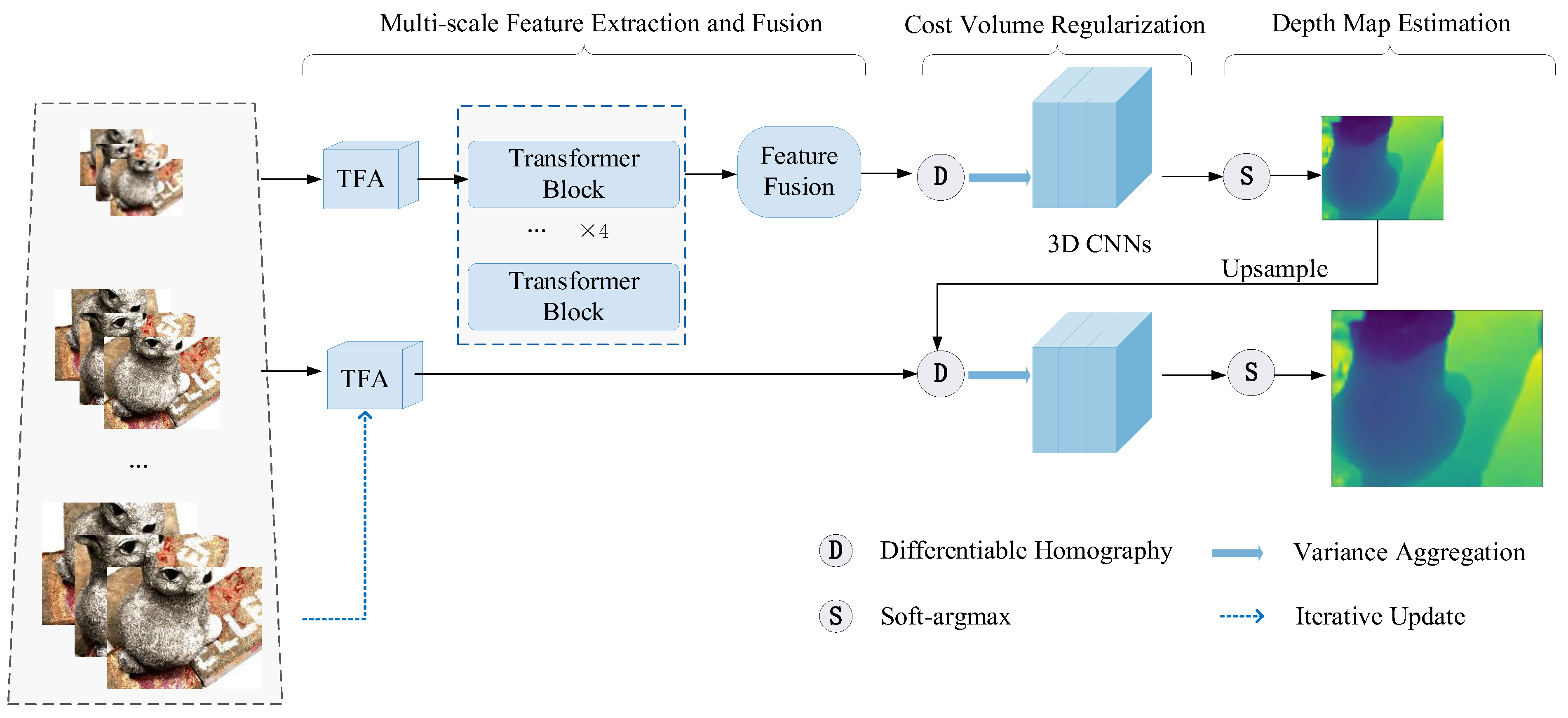
3. Methods
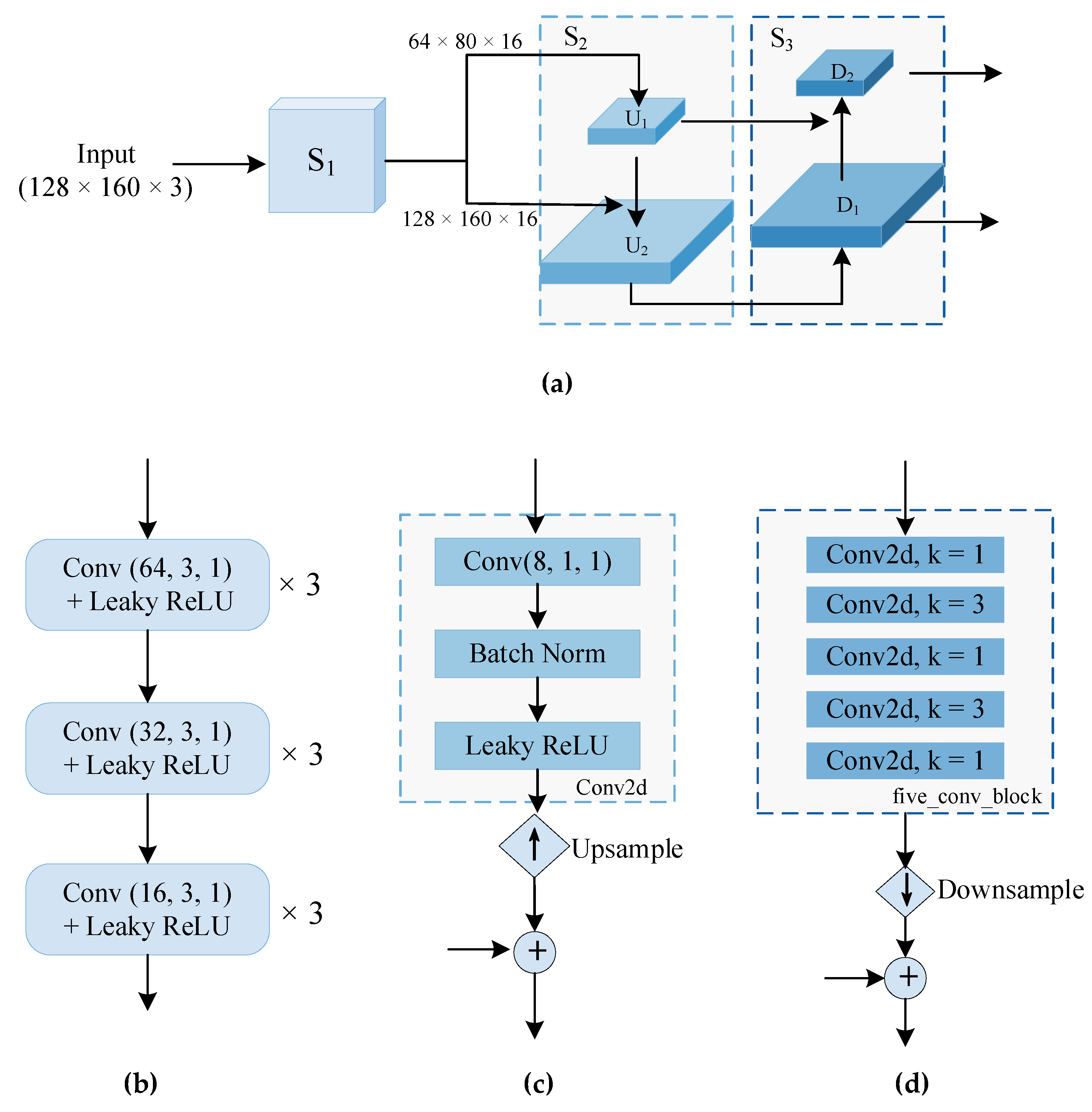
3.1. Image Feature Pyramid
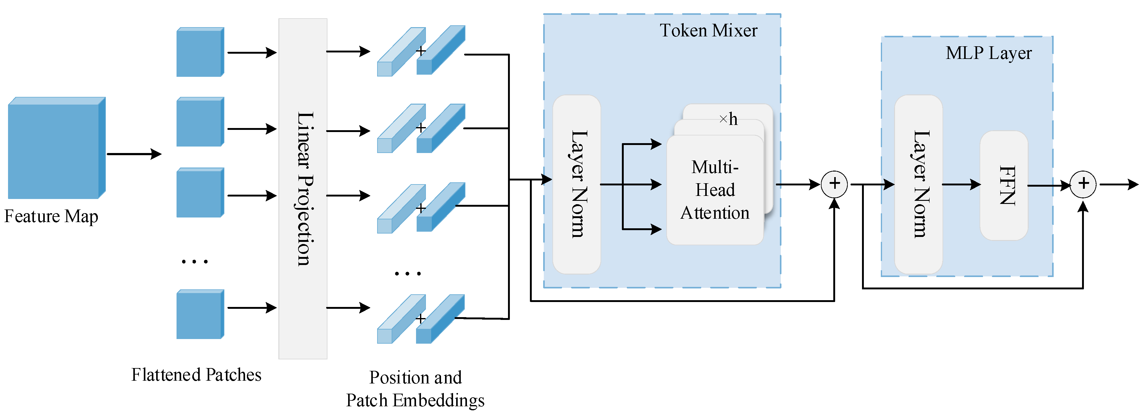
3.2. Transformer for Coarse Feature Fusion
3.2.1. Transformer Block
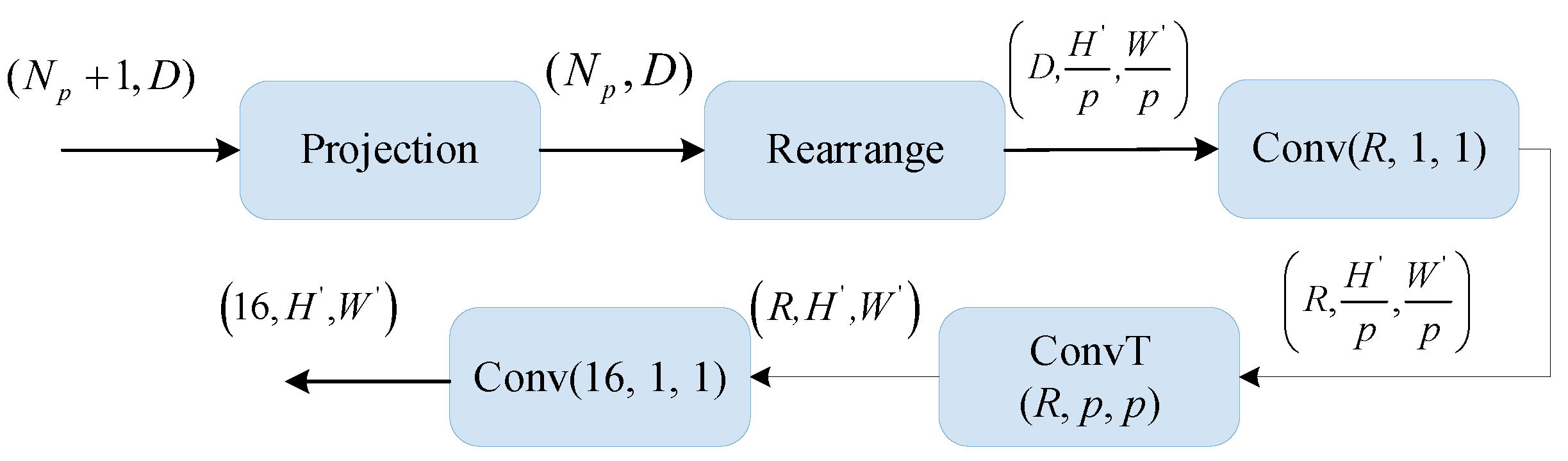
3.2.2. Image-like Feature Fusion Module
3.3. Depth Inference for MVS
3.4. Loss Function
4. Experiments
4.1. Dataset
4.2. Metrics
4.3. Implementation Details
4.4. Experimental Performance
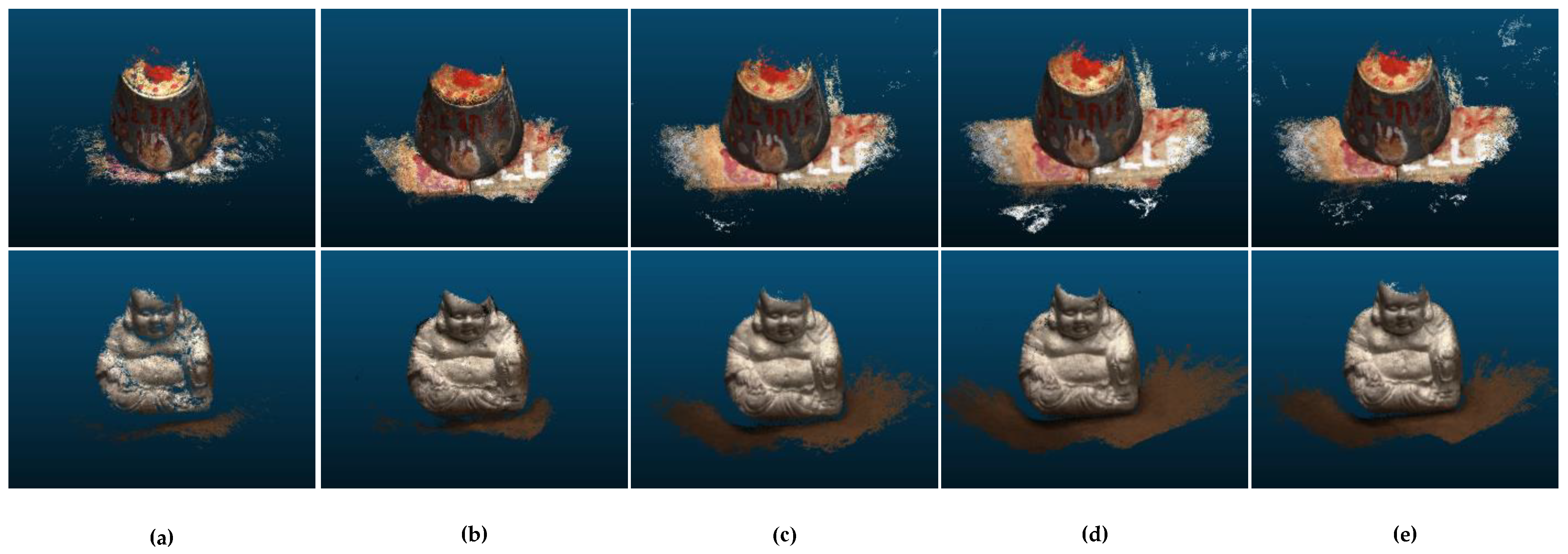
4.4.1. Results on DTU Dataset
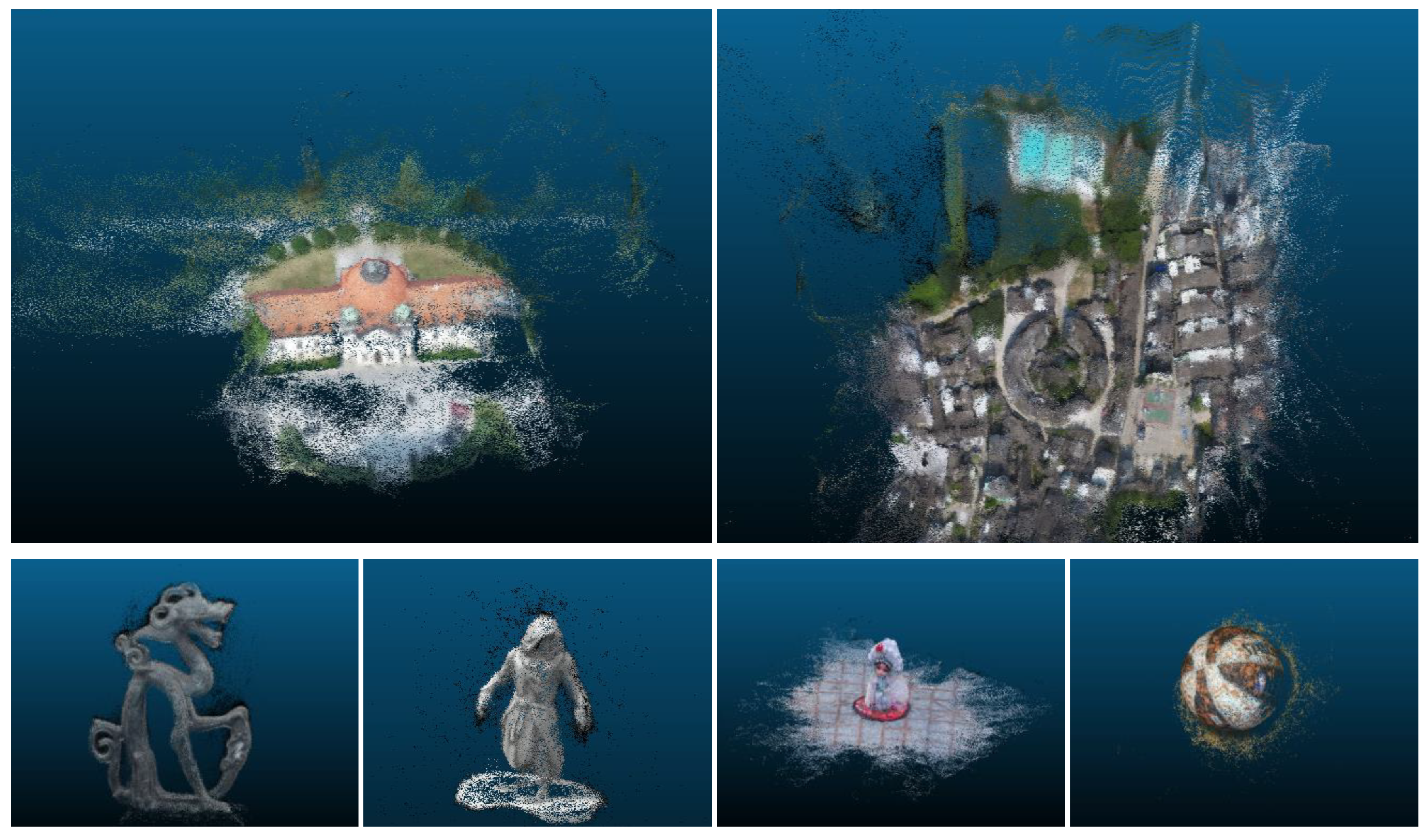
4.4.2. Results on BlendedMVS Dataset
4.5. Ablation Study
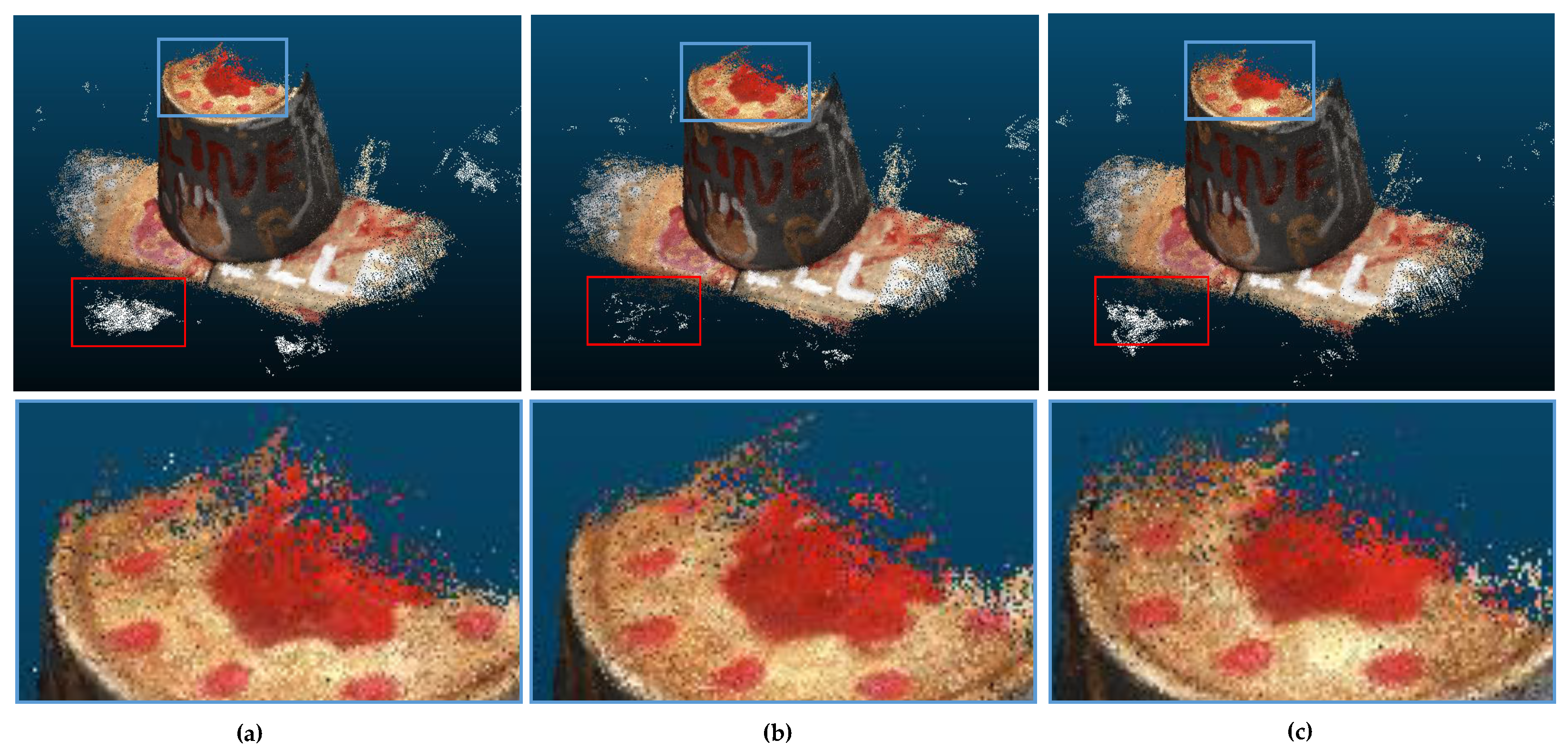
4.5.1. Effectiveness of Different Components
4.5.2. Evaluation Patch Size Settings
4.5.3. Explore on Learnable Token
4.5.4. Number of Different Transformer Blocks
4.5.5. Extension on Different Resolution Images
5. Conclusions
Author Contributions
Funding
Institutional Review Board Statement
Informed Consent Statement
Data Availability Statement
Conflicts of Interest
References
- Zhao, J.; Liu, S.; Li, J. Research and Implementation of Autonomous Navigation for Mobile Robots Based on SLAM Algorithm under ROS. Sensors 2022, 22, 4172. [Google Scholar] [CrossRef] [PubMed]
- Li, M.; Du, Z.; Ma, X.; Dong, W.; Gao, Y. A robot hand-eye calibration method of line laser sensor based on 3D reconstruction. Robot. Comput. Integr. Manuf. 2021, 71, 102136. [Google Scholar] [CrossRef]
- Han, L.; Zheng, T.; Zhu, Y.; Xu, L.; Fang, L. Live Semantic 3D Perception for Immersive Augmented Reality. IEEE Trans. Vis. Comput. Graph. 2020, 26, 2012–2022. [Google Scholar] [CrossRef]
- Barreto, M.A.; Perez-Gonzalez, J.; Herr, H.M.; Huegel, J.C. ARACAM: A RGB-D Multi-View Photogrammetry System for Lower Limb 3D Reconstruction Applications. Sensors 2022, 22, 2443. [Google Scholar] [CrossRef] [PubMed]
- Masiero, A.; Chiabrando, F.; Lingua, A.M.; Marino, B.G.; Fissore, F.; Guarnieri, A.; Vettore, A. 3D MODELING of GIRIFALCO FORTRESS. ISPRS Ann. Photogramm. Remote Sens. Spat. Inf. Sci. 2019, 42, 473–478. [Google Scholar] [CrossRef]
- Hirschmüller, H. Stereo processing by semiglobal matching and mutual information. IEEE Trans. Pattern Anal. Mach. Intell. 2008, 30, 328–341. [Google Scholar] [CrossRef]
- Schonberger, J.L.; Frahm, J.M. Structure-from-Motion Revisited. In Proceedings of the IEEE Computer Society Conference on Computer Vision and Pattern Recognition, Las Vegas, NV, USA, 27–30 June 2016; pp. 4104–4113. [Google Scholar]
- Aanæs, H.; Jensen, R.R.; Vogiatzis, G.; Tola, E.; Dahl, A.B. Large-Scale Data for Multiple-View Stereopsis. Int. J. Comput. Vis. 2016, 120, 153–168. [Google Scholar] [CrossRef]
- Knapitsch, A.; Park, J.; Zhou, Q.Y.; Koltun, V. Tanks and temples: Benchmarking large-scale scene reconstruction. ACM Trans. Graph. 2017, 36, 1–13. [Google Scholar] [CrossRef]
- Yao, Y.; Luo, Z.; Li, S.; Fang, T.; Quan, L. MVSNet: Depth inference for unstructured multi-view stereo. In Proceedings of the European Conference on Computer Vision, Munich, Germany, 8–14 September 2018; Volume 11212 LNCS, pp. 785–801. [Google Scholar]
- Yang, J.; Mao, W.; Alvarez, J.M.; Liu, M. Cost volume pyramid based depth inference for multi-view stereo. In Proceedings of the IEEE Computer Society Conference on Computer Vision and Pattern Recognition, Seattle, WA, USA, 16–18 June 2020; pp. 4876–4885. [Google Scholar]
- Yu, A.; Guo, W.; Liu, B.; Chen, X.; Wang, X.; Cao, X.; Jiang, B. Attention aware cost volume pyramid based multi-view stereo network for 3D reconstruction. ISPRS J. Photogramm. Remote Sens. 2021, 175, 448–460. [Google Scholar] [CrossRef]
- Wei, Z.; Zhu, Q.; Min, C.; Chen, Y.; Wang, G. AA-RMVSNet: Adaptive Aggregation Recurrent Multi-view Stereo Network. In Proceedings of the IEEE International Conference on Computer Vision, Montreal, QC, Canada, 10–17 October 2021; pp. 6167–6176. [Google Scholar]
- Gu, X.; Fan, Z.; Zhu, S.; Dai, Z.; Tan, F.; Tan, P. Cascade Cost Volume for High-Resolution Multi-View Stereo and Stereo Matching. In Proceedings of the IEEE Computer Society Conference on Computer Vision and Pattern Recognition, Seattle, WA, USA, 13–19 June 2020; pp. 2492–2501. [Google Scholar]
- Ma, X.; Gong, Y.; Wang, Q.; Huang, J.; Chen, L.; Yu, F. EPP-MVSNet: Epipolar-assembling based Depth Prediction for Multi-view Stereo. In Proceedings of the 2021 IEEE/CVF International Conference on Computer Vision (ICCV), Montreal, QC, Canada, 10–17 October 2021; pp. 5712–5720. [Google Scholar] [CrossRef]
- Wang, F.; Galliani, S.; Vogel, C.; Speciale, P.; Pollefeys, M. PatchMatchNet: Learned multi-view patchmatch stereo. In Proceedings of the 2021 IEEE/CVF Conference on Computer Vision and Pattern Recognition (CVPR), Virtual, 19–25 June 2021; pp. 14189–14198. [Google Scholar] [CrossRef]
- Yan, J.; Wei, Z.; Yi, H.; Ding, M.; Zhang, R.; Chen, Y.; Wang, G.; Tai, Y.W. Dense Hybrid Recurrent Multi-view Stereo Net with Dynamic Consistency Checking. In Proceedings of the European Conference on Computer Vision, Glasgow, UK, 23–28 August 2020; Volume 12349 LNCS, pp. 674–689. [Google Scholar]
- Vaswani, A.; Shazeer, N.; Parmar, N.; Uszkoreit, J.; Jones, L.; Gomez, A.N.; Kaiser, Ł.; Polosukhin, I. Attention is all you need. Adv. Neural Inf. Process Syst. 2017, 2017-Decem, 5999–6009. [Google Scholar]
- Dosovitskiy, A.; Beyer, L.; Kolesnikov, A.; Weissenborn, D.; Zhai, X.; Unterthiner, T.; Dehghani, M.; Minderer, M.; Heigold, G.; Gelly, S.; et al. An image is worthI 16 × 16 words: Transformers for image recognition at scale. In Proceedings of the International Conference on Learning Representations, Vienna, Austria, 4 May 2021. [Google Scholar]
- He, C.; Li, R.; Li, S.; Zhang, L. Voxel Set Transformer: A Set-to-Set Approach to 3D Object Detection from Point Clouds. In Proceedings of the IEEE Computer Society Conference on Computer Vision and Pattern Recognition, New Orleans, LA, USA, 18–24 June 2022; pp. 8417–8427. [Google Scholar]
- Xu, L.; Ouyang, W.; Bennamoun, M.; Boussaid, F.; Xu, D. Multi-class Token Transformer for Weakly Supervised Semantic Segmentation. In Proceedings of the IEEE Computer Society Conference on Computer Vision and Pattern Recognition, New Orleans, LA, USA, 18–24 June 2022; pp. 4310–4319. [Google Scholar]
- Ding, Y.; Yuan, W.; Zhu, Q.; Zhang, H.; Liu, X.; Wang, Y.; Liu, X. TransMVSNet: Global Context-aware Multi-view Stereo Network with Transformers. In Proceedings of the IEEE Computer Society Conference on Computer Vision and Pattern Recognition, New Orleans, LA, USA, 18–24 June 2022; pp. 8585–8594. [Google Scholar]
- Zhu, J.; Peng, B.; Li, W.; Shen, H.; Zhang, Z.; Lei, J. Multi-View Stereo with Transformer. arXiv 2021, arXiv:2112.00336. [Google Scholar]
- Wang, X.; Zhu, Z.; Qin, F.; Ye, Y.; Huang, G.; Chi, X.; He, Y.; Wang, X. MVSTER: Epipolar Transformer for Efficient Multi-View Stereo. arXiv 2022, arXiv:2204.07346. [Google Scholar]
- Liao, J.; Ding, Y.; Shavit, Y.; Huang, D.; Ren, S.; Guo, J.; Feng, W.; Zhang, K. WT-MVSNet: Window-based Transformers for Multi-view Stereo. arXiv 2022, arXiv:2205.14319. [Google Scholar]
- Furukawa, Y.; Curless, B.; Seitz, S.M.; Szeliski, R. Towards Internet-scale Multi-view Stereo. In Proceedings of the IEEE Computer Society Conference on Computer Vision and Pattern Recognition, San Francisco, CA, USA, 13–18 June 2010; pp. 1434–1441. [Google Scholar]
- Yang, M.D.; Chao, C.F.; Huang, K.S.; Lu, L.Y.; Chen, Y.P. Image-based 3D scene reconstruction and exploration in augmented reality. Autom. Constr. 2013, 33, 48–60. [Google Scholar] [CrossRef]
- Fuentes-Pacheco, J.; Ruiz-Ascencio, J.; Rendón-Mancha, J.M. Visual simultaneous localization and mapping: A survey. Artif. Intell. Rev. 2015, 43, 55–81. [Google Scholar] [CrossRef]
- Redmon, J.; Farhadi, A. YOLO v.3. arXiv 2018, arXiv:1804.02767. [Google Scholar]
- Godard, C.; Aodha, O.M.; Firman, M.; Brostow, G. Digging into self-supervised monocular depth estimation. Proc. IEEE Int. Conf. Comput. Vis. 2019, 2019-Octob, 3827–3837. [Google Scholar] [CrossRef]
- Rozumnyi, D.; Oswald, M.; Ferrari, V.; Matas, J.; Pollefeys, M. DeFMO: Deblurring and shape recovery of fast moving objects. arXiv 2020, arXiv:2012.00595. [Google Scholar]
- Ji, M.; Gall, J.; Zheng, H.; Liu, Y.; Fang, L. SurfaceNet: An End-to-End 3D Neural Network for Multiview Stereopsis. Proc. IEEE Int. Conf. Comput. Vis. 2017, 2017-Octob, 2326–2334. [Google Scholar] [CrossRef]
- Kar, A.; Häne, C.; Malik, J. Learning a multi-view stereo machine. Adv. Neural Inf. Process. Syst. 2017, 2017-Decem, 365–376. [Google Scholar]
- Touvron, H.; Massa, F.; Cord, M.; Sablayrolles, A. Training data-efficient image transformers & distillation through attention. arXiv 2012, arXiv:2012.12877. [Google Scholar]
- Liu, Z.; Lin, Y.; Cao, Y.; Hu, H.; Wei, Y.; Zhang, Z.; Lin, S.; Guo, B. Swin Transformer: Hierarchical Vision Transformer using Shifted Windows. In Proceedings of the 2021 IEEE/CVF International Conference on Computer Vision (ICCV), Montreal, QC, Canada, 10–17 October 2021; pp. 9992–10002. [Google Scholar] [CrossRef]
- Ronneberger, O.; Fischer, P.; Brox, T. UNet: Convolutional Networks for Biomedical Image Segmentation. In Proceedings of the International Conference on Medical Image Computing and Computer Assisted Intervention, Munich, Germany, 5–9 October 2015; pp. 234–241. [Google Scholar]
- Devlin, J.; Chang, M.W.; Lee, K.; Toutanova, K. BERT: Pre-training of deep bidirectional transformers for language understanding. In Proceedings of the 2019 Conference of the North American Chapter of the Association for Computational Linguistics: Human Language Technologies—Proceedings of the Conference, Minneapolis, MN, USA, 2–7 June 2019; Volume 1, pp. 4171–4186. [Google Scholar]
- Yao, Y.; Luo, Z.; Li, S.; Zhang, J.; Ren, Y.; Zhou, L.; Fang, T.; Quan, L. BlendedMVS: A large-scale dataset for generalized multi-view stereo networks. In Proceedings of the IEEE Computer Society Conference on Computer Vision and Pattern Recognition, Seattle, WA, USA, 13–19 June 2020; pp. 1787–1796. [Google Scholar]
- Seitz, S.M.; Diebel, J.; Scharstein, D.; Szeliski, R. A Comparison and Evaluation of Multi-View Stereo Reconstruction Algorithms. In Proceedings of the 2006 IEEE Computer Society Conference on Computer Vision and Pattern Recognition (CVPR’06), New York, NY, USA, 17–22 June 2006; pp. 519–528. [Google Scholar]
- Kingma, D.P.; Ba, J.L. Adam: A method for stochastic optimization. In Proceedings of the 3rd International Conference on Learning Representations, ICLR 2015—Conference Track Proceedings, San Diego, CA, USA, 7–9 May 2015; pp. 1–15. [Google Scholar]
- Merrell, P.; Akbarzadeh, A.; Wang, L.; Mordohai, P.; Frahm, J.M.; Yang, R.; Nistér, D.; Pollefeys, M. Real-time visibility-based fusion of depth maps. In Proceedings of the 2007 IEEE 11th International Conference on Computer Vision, Rio de Janeiro, Brazil, 14–21 October 2007. [Google Scholar] [CrossRef]


| Method | Acc. (mm) | Comp. (mm) | Overall (mm) |
|---|---|---|---|
| Colmap [7] | 6.5778 | 10.1405 | 8.2930 |
| AA-RMVSNet [13] | 0.8207 | 3.4115 | 2.1161 |
| CasMVSNet [14] | 1.4045 | 1.6096 | 1.5071 |
| CVP-MVSNet [11] | 1.1964 | 1.0569 | 1.1267 |
| AACVP-MVSNet [12] | 1.1329 | 0.8814 | 1.0071 |
| MVSTER [24] | 2.6132 | 1.9704 | 2.2918 |
| TransMVS [22] | 1.0248 | 1.3075 | 1.1662 |
| Ours | 0.9296 | 1.0120 | 0.9708 |
| Model Settings | Mean Distance | ||||
|---|---|---|---|---|---|
| TFA | Transformer | Acc. | Comp. | Overall | |
| (a) | 1.1964 | 1.0569 | 1.1267 | ||
| (b) | √ | 0.9635 | 1.0257 | 0.9946 | |
| (c) | √ | √ | 0.9296 | 1.0120 | 0.9708 |
| Acc. | Comp. | Overall | |
|---|---|---|---|
| patch size = 8 | 1.0182 | 1.1022 | 1.0602 |
| patch size = 4 | 0.9296 | 1.0120 | 0.9708 |
| patch size = 2 | 0.9465 | 1.0237 | 0.9851 |
| -cls | ignore | add | map | |
|---|---|---|---|---|
| Acc. | 0.9287 | 0.9296 | 0.9856 | 0.9724 |
| Comp. | 1.0363 | 1.0120 | 1.0692 | 1.0505 |
| Overall | 0.9825 | 0.9708 | 1.0274 | 1.0114 |
| T | Acc. | Comp. | Overall |
|---|---|---|---|
| 6 | 0.9731 | 1.0575 | 1.0153 |
| 4 | 0.9296 | 1.0120 | 0.9708 |
| 2 | 1.0148 | 1.0824 | 1.0486 |
| Image Size | Acc. | Comp. | Overall |
|---|---|---|---|
| 160 × 128 | 0.9296 | 1.0120 | 0.9708 |
| 320 × 256 | 0.7695 | 1.0163 | 0.8929 |
| 640 × 512 | 0.5348 | 1.2394 | 0.8871 |
| 1280 × 1024 | 0.4089 | 0.9584 | 0.6836 |
Publisher’s Note: MDPI stays neutral with regard to jurisdictional claims in published maps and institutional affiliations. |
© 2022 by the authors. Licensee MDPI, Basel, Switzerland. This article is an open access article distributed under the terms and conditions of the Creative Commons Attribution (CC BY) license (https://creativecommons.org/licenses/by/4.0/).
Share and Cite
Jia, R.; Chen, X.; Cui, J.; Hu, Z. MVS-T: A Coarse-to-Fine Multi-View Stereo Network with Transformer for Low-Resolution Images 3D Reconstruction. Sensors 2022, 22, 7659. https://doi.org/10.3390/s22197659
Jia R, Chen X, Cui J, Hu Z. MVS-T: A Coarse-to-Fine Multi-View Stereo Network with Transformer for Low-Resolution Images 3D Reconstruction. Sensors. 2022; 22(19):7659. https://doi.org/10.3390/s22197659
Chicago/Turabian StyleJia, Ruiming, Xin Chen, Jiali Cui, and Zhenghui Hu. 2022. "MVS-T: A Coarse-to-Fine Multi-View Stereo Network with Transformer for Low-Resolution Images 3D Reconstruction" Sensors 22, no. 19: 7659. https://doi.org/10.3390/s22197659
APA StyleJia, R., Chen, X., Cui, J., & Hu, Z. (2022). MVS-T: A Coarse-to-Fine Multi-View Stereo Network with Transformer for Low-Resolution Images 3D Reconstruction. Sensors, 22(19), 7659. https://doi.org/10.3390/s22197659