
A Probabilistic Bayesian Parallel Deep Learning Framework for Wind Turbine Bearing Fault Diagnosis

Abstract
1. Introduction
- (1)
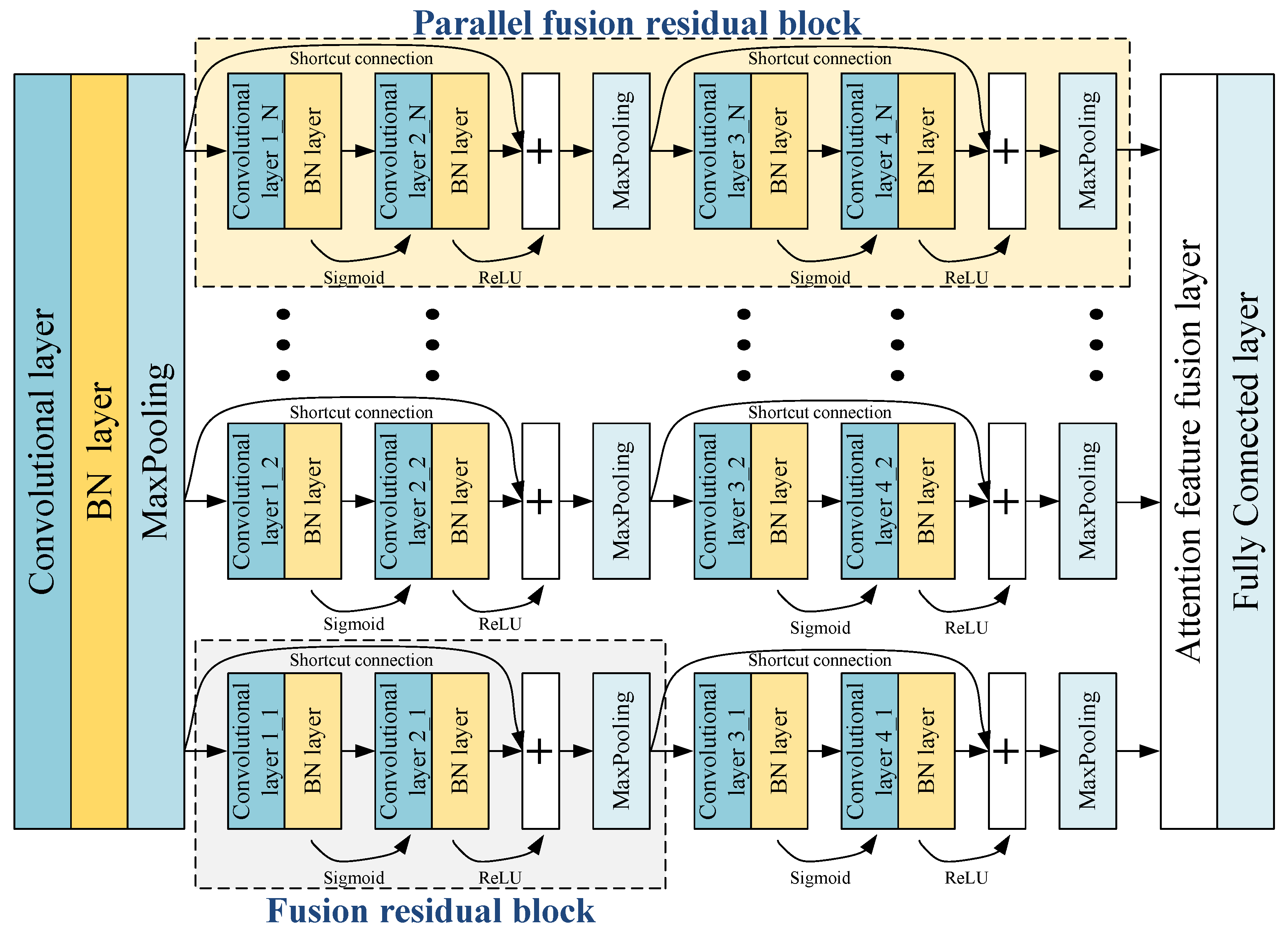
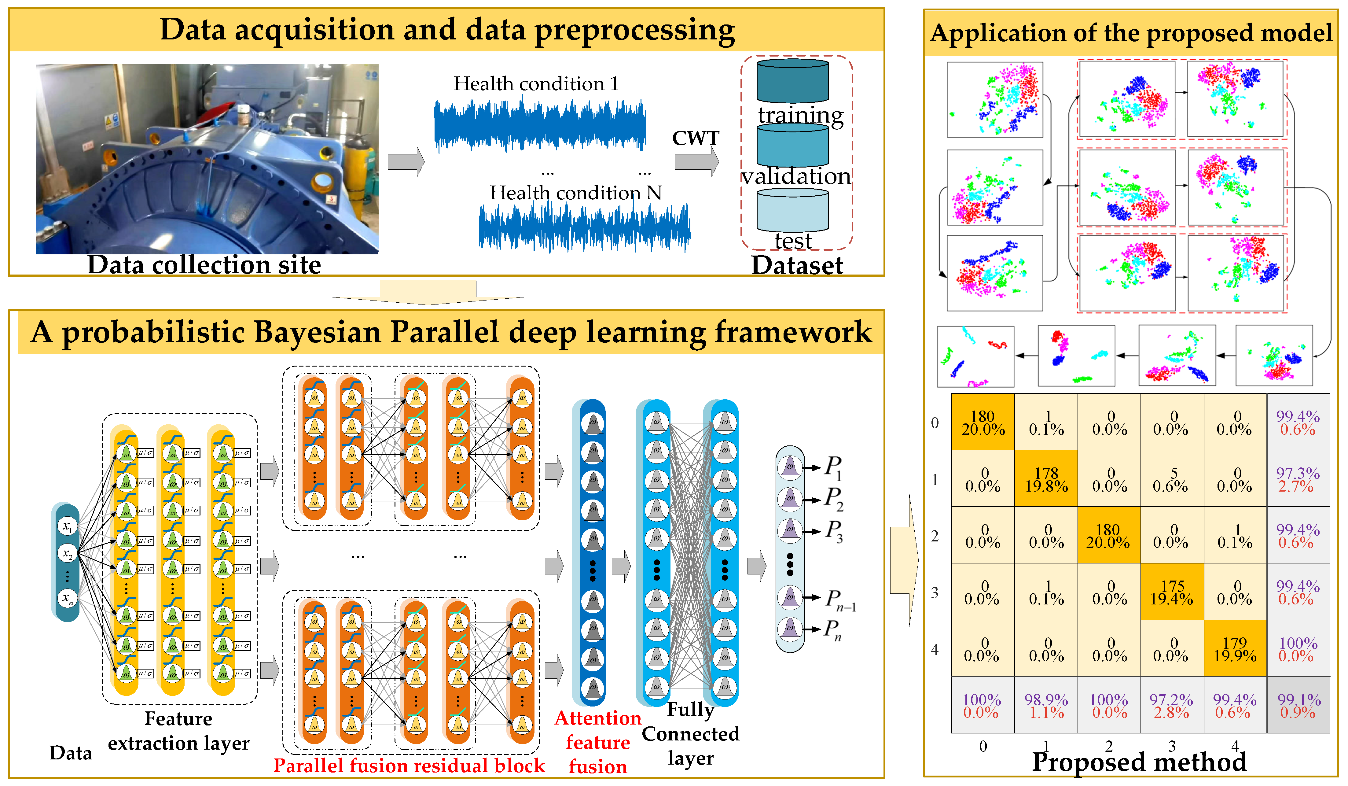
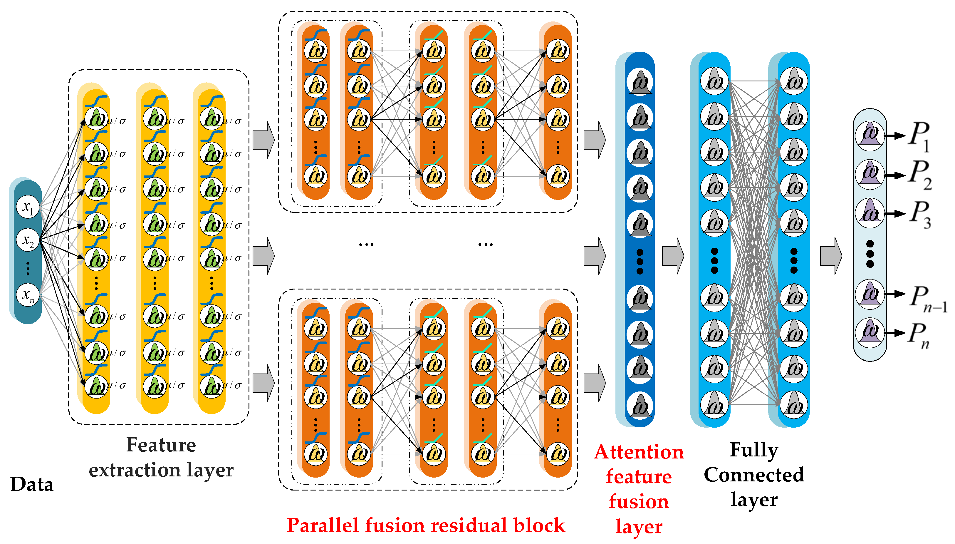
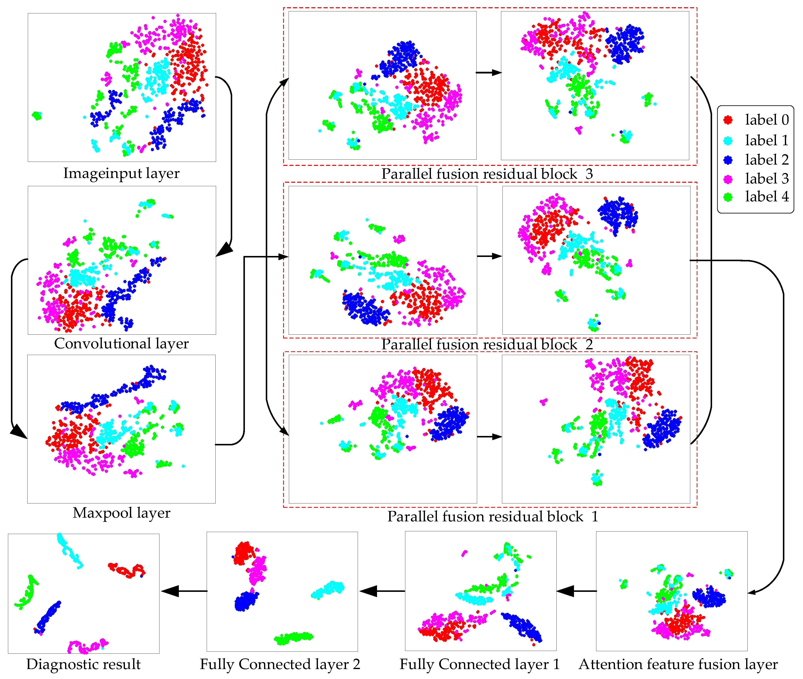
- The PDL framework is constructed to enhance the feature learning ability. Multiple parallel fusion residual blocks (PFRBs) are parallelized, which can enable the fault diagnosis performance. The PDL framework can adaptively select the number of PFRBs according to the characteristics of the dataset.
- (2)
- A probabilistic Bayesian parallel deep learning framework fault diagnosis method is proposed under the framework of probabilistic Bayesian deep learning for the uncertainty perception of faults.
- (3)
- Taking the fault signal of the gearbox output shaft bearing of a wind turbine in a wind farm as an example, it is proved that the proposed method has high accuracy and confidence in the diagnosis results. It exhibits excellent performance in the fault identification of wind turbine bearings.
2. Parallel Deep Learning Framework
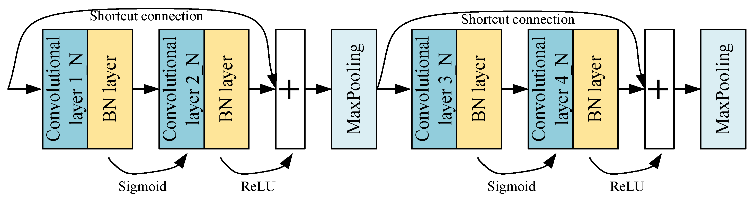
2.1. Parallel Fusion Residual Block
2.2. Attention Feature Fusion Layer
3. Proposed Method
3.1. A Probabilistic Bayesian Parallel Deep Learning Framework
3.2. Variational Inference
3.3. Uncertainty Analysis
4. Case Studies and Results
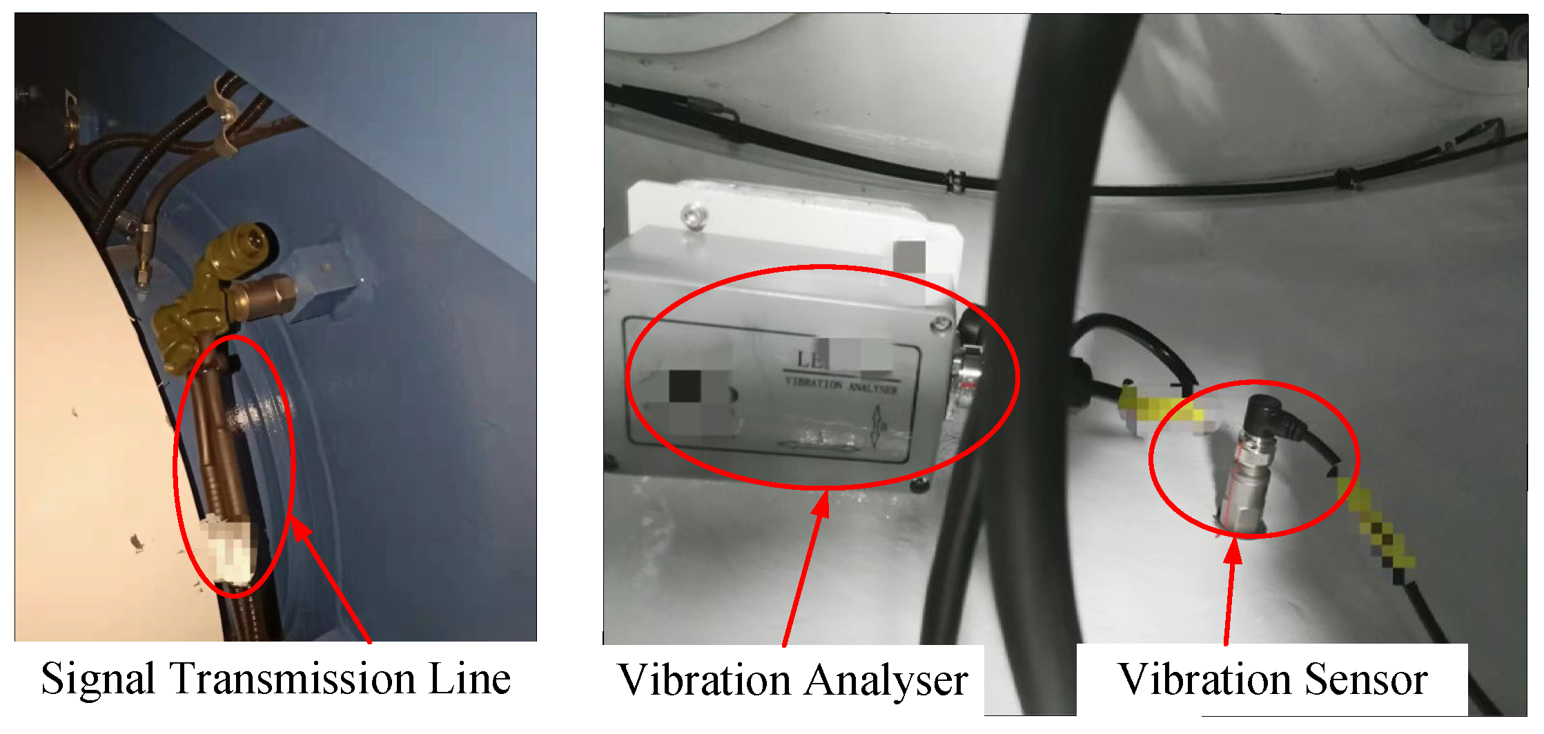
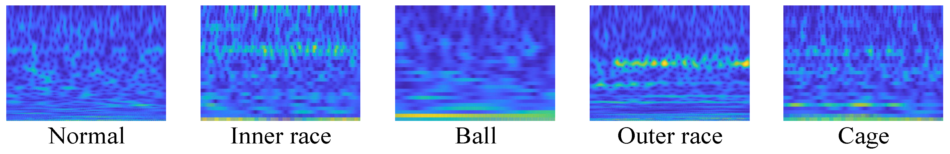
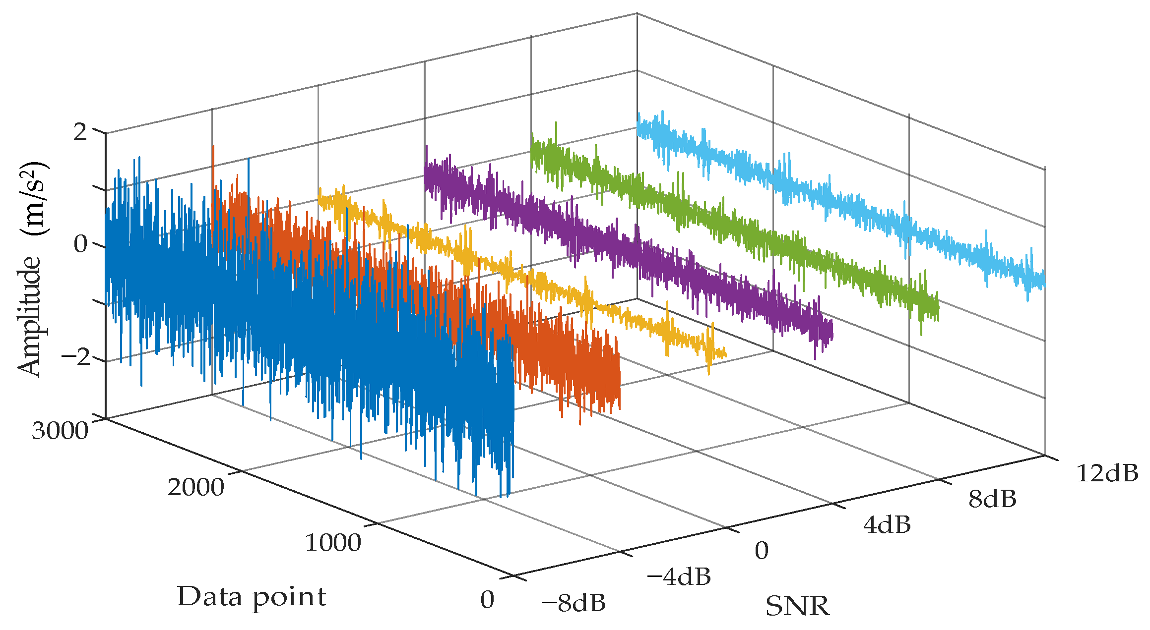
4.1. Experimental Setup
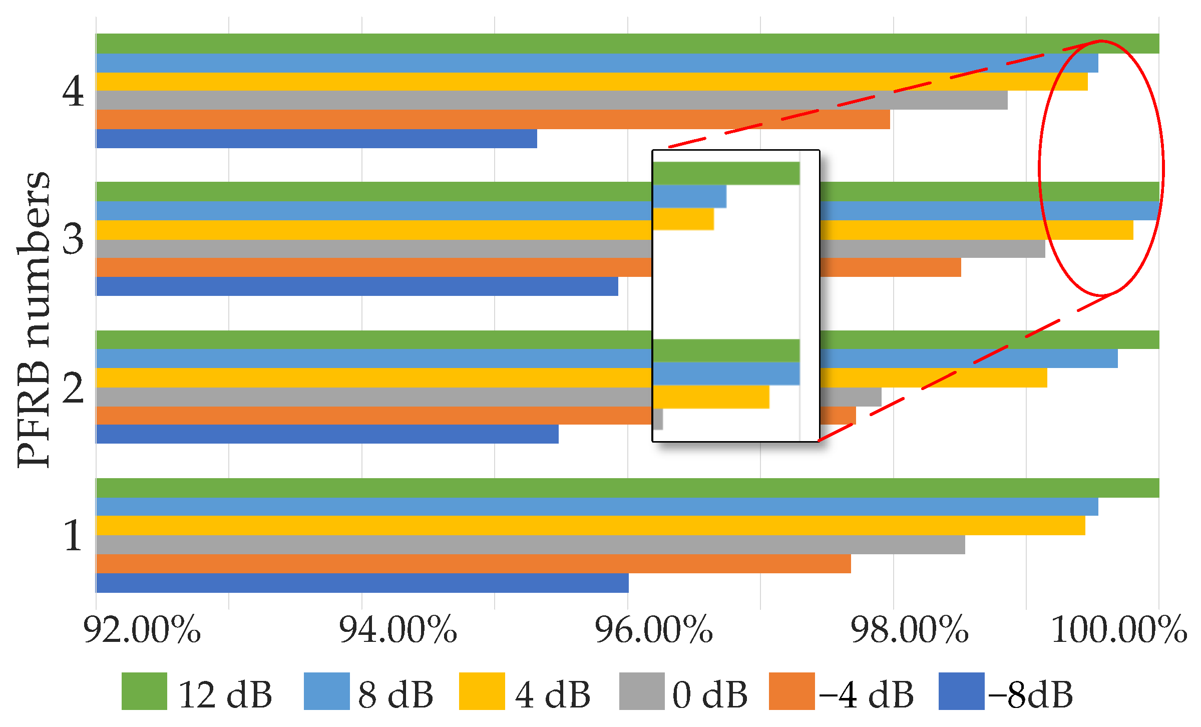
4.2. Experimental Results and Discussion
5. Conclusions
- (1)
- A structure of PFRBs is constructed to enrich high-level feature data. The fault feature extraction ability of the PDL framework is improved without increasing the network parameters. Through the attention mechanism, useful information is identified by the network in the extracted features.
- (2)
- Based on the PDL framework, the hyperparameters of the network are parameterized, providing the probability distribution of all hyperparameters, which makes the neural network uncertain. A probabilistic BayesianPDL framework diagnostic method specially applied to wind turbines bearing faults is designed.
- (3)
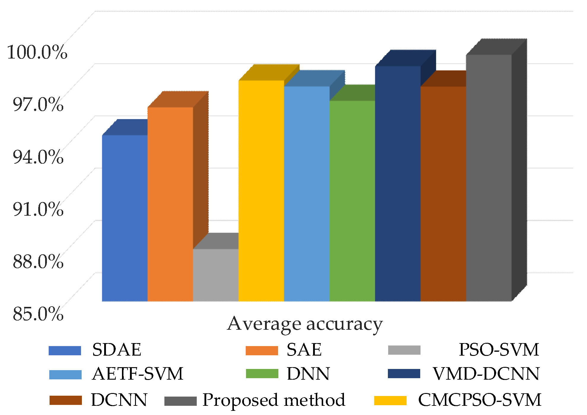
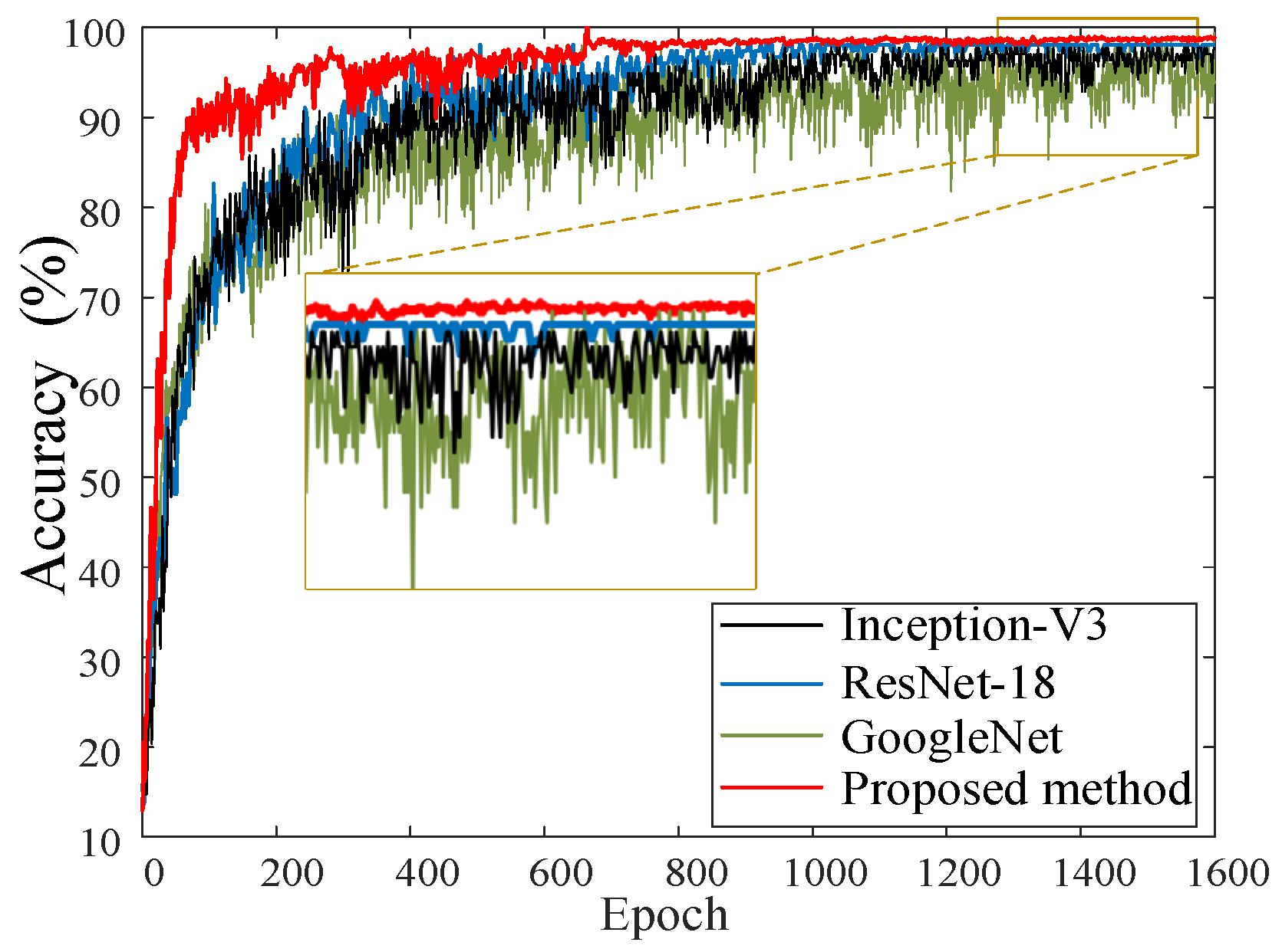
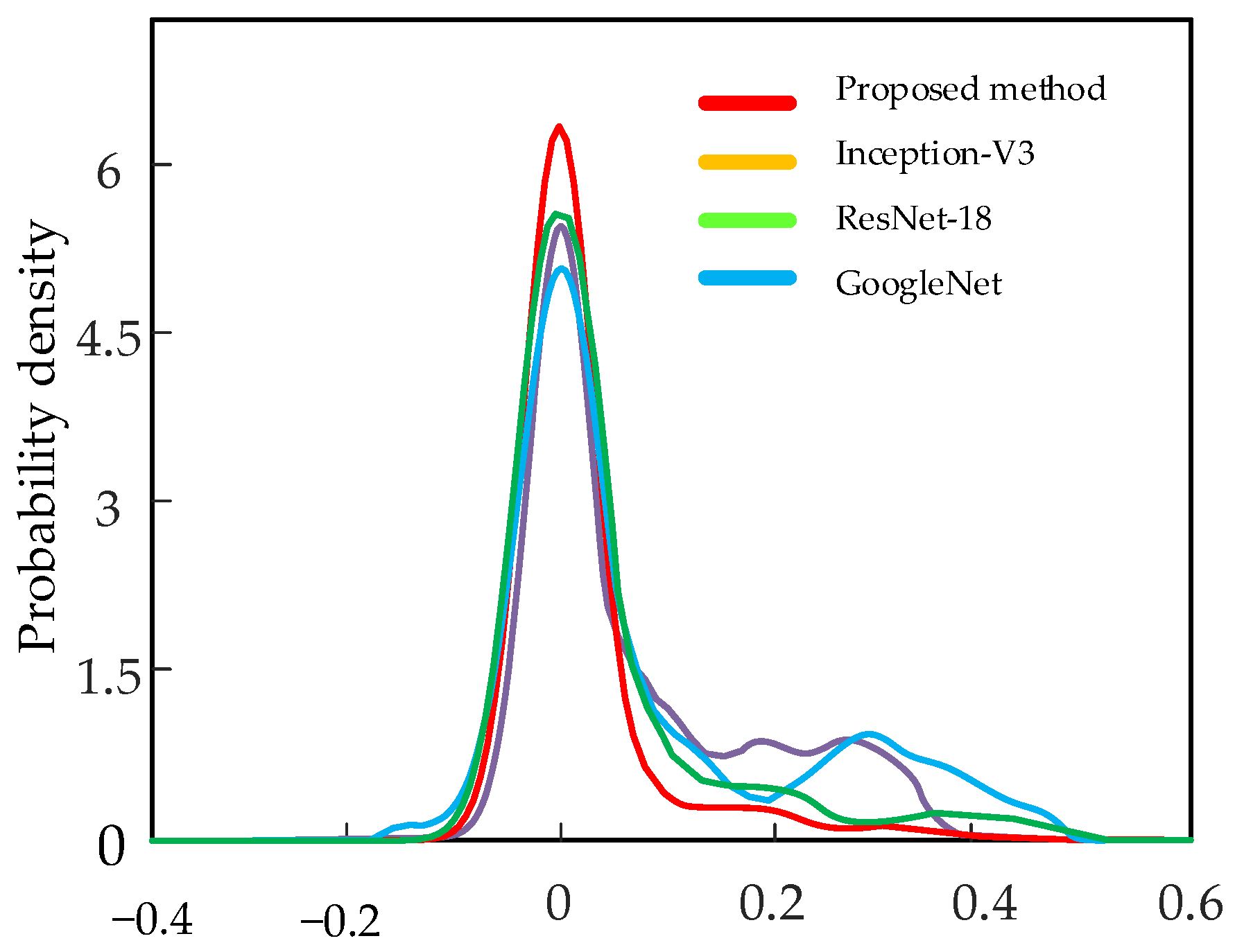
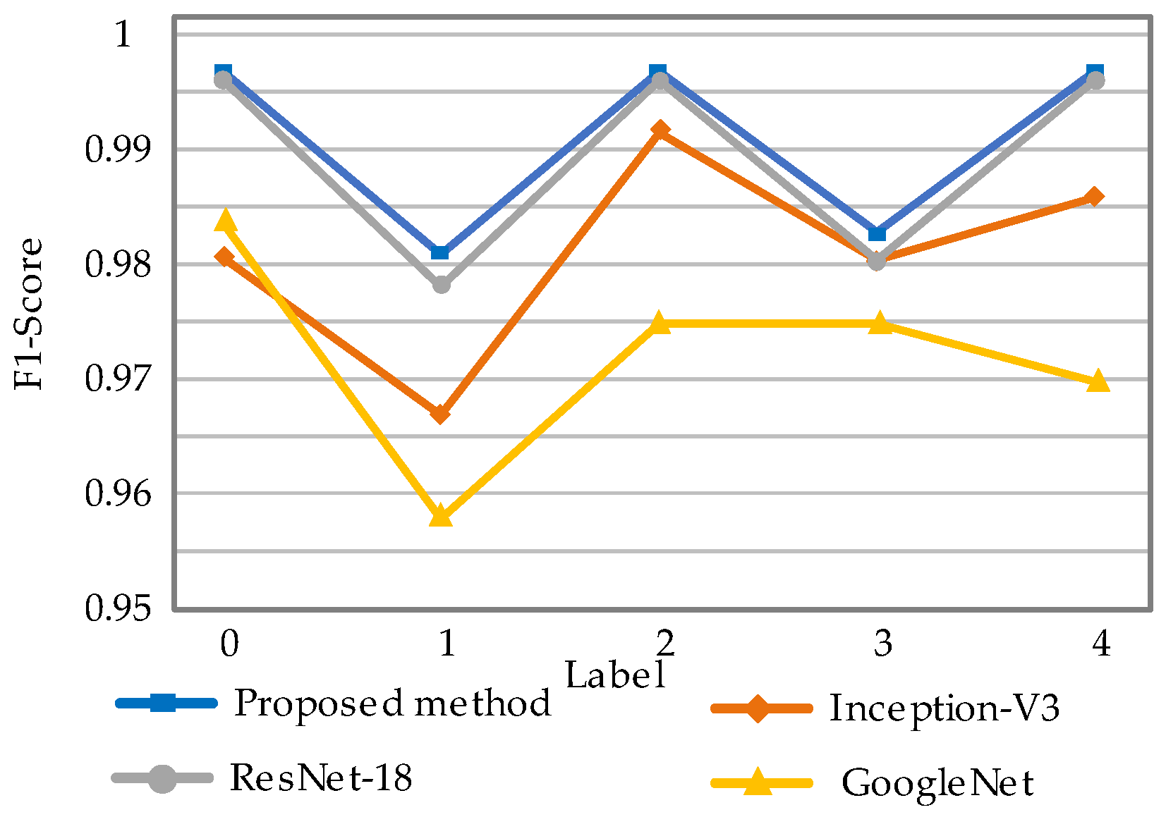
- Compared with other non-probabilistic models, the proposed method has a higher diagnostic performance. Compared with other probability models, the diagnostic results of the proposed method have higher accuracy and confidence.
Author Contributions
Funding
Institutional Review Board Statement
Informed Consent Statement
Data Availability Statement
Conflicts of Interest
References
- Global Wind Report 2019; Global Wind Energy Council: Brussels, Belgium, 2020.
- Zhang, K.; Tang, B.; Deng, L.; Tan, Q.; Yu, H. A fault diagnosis method for wind turbines gearbox based on adaptive loss weighted meta-ResNet under noisy labels. Mech. Syst. Signal Process. 2021, 161, 107963. [Google Scholar] [CrossRef]
- Wang, L.; Ma, Y.; Rui, X. Research on Fault Diagnosis Method of Wind Turbine Bearing Based on Deep belief Network. IOP Conf. Ser. Mater. Sci. Eng. 2019, 677, 032025. [Google Scholar] [CrossRef]
- Zhang, Y.; Liu, W.; Gu, H.; Alexisa, A.; Jiang, X. A novel wind turbine fault diagnosis based on deep transfer learning of improved residual network and multi-target data. Meas. Sci. Technol. 2022, 33, 095007. [Google Scholar] [CrossRef]
- Lu, L.; He, Y.; Ruan, Y.; Yuan, W. An optimized stacked diagnosis structure for fault diagnosis of wind turbine planetary gearbox. Meas. Sci. Technol. 2021, 32, 075102. [Google Scholar] [CrossRef]
- Teng, W.; Ding, X.; Tang, S.; Xu, J.; Shi, B.; Liu, Y. Vibration Analysis for Fault Detection of Wind Turbine Drivetrains—A Comprehensive Investigation. Sensors 2021, 21, 1686. [Google Scholar] [CrossRef] [PubMed]
- Xie, S.; Li, Y.; Tan, H.; Liu, R.; Zhang, F. Multi-scale and multi-layer perceptron hybrid method for bearings fault diagnosis. Int. J. Mech. Sci. 2022, 235, 107708. [Google Scholar] [CrossRef]
- Li, N.; Zhou, R.; Hu, Q.; Liu, X. Mechanical fault diagnosis based on redundant second generation wavelet packet transform, neighborhood rough set and support vector machine. Mech. Syst. Signal Process. 2012, 28, 608–621. [Google Scholar] [CrossRef]
- Verbert, K.; Babuška, R.; De Schutter, B. Bayesian and Dempster-Shafer reasoning for knowledge-based fault diagnosis—A comparative study. Eng. Appl. Artif. Intell. 2017, 60, 136–150. [Google Scholar] [CrossRef]
- Jin, Z.; He, D.; Wei, Z. Intelligent fault diagnosis of train axle box bearing based on parameter optimization VMD and improved DBN. Eng. Appl. Artif. Intell. 2022, 110, 104713. [Google Scholar] [CrossRef]
- Yeh, C.; Lin, M.; Lin, C.; Yu, C.; Chen, M. Machine Learning for Long Cycle Maintenance Prediction of Wind Turbine. Sensors 2019, 19, 1671. [Google Scholar] [CrossRef]
- Li, J.; Yao, X.; Wang, X.; Yu, Q.; Zhang, Y. Multiscale local features learning based on BP neural network for rolling bearing intelligent fault diagnosis. Measurement 2020, 153, 107419. [Google Scholar] [CrossRef]
- Xu, T.; Ji, J.; Kong, X.; Zou, F.; Wang, W.; Cherifi, H. Bearing Fault Diagnosis in the Mixed Domain Based on Crossover-Mutation Chaotic Particle Swarm. Complexity 2021, 2021, 6632187. [Google Scholar] [CrossRef]
- Xu, Z.; Mei, X.; Wang, X.; Yue, M.; Jin, J.; Yang, Y.; Li, C. Fault diagnosis of wind turbine bearing using a multi-scale convolutional neural network with bidirectional long short term memory and weighted majority voting for multi-sensors. Renew. Energy 2022, 182, 615–626. [Google Scholar] [CrossRef]
- Kong, Y.; Qin, Z.; Wang, T.; Han, Q.; Chu, F. An enhanced sparse representation-based intelligent recognition method for planet bearing fault diagnosis in wind turbines. Renew. Energy 2021, 173, 987–1004. [Google Scholar] [CrossRef]
- Xu, Z.; Li, C.; Yang, Y. Fault diagnosis of rolling bearing of wind turbines based on the Variational Mode Decomposition and Deep Convolutional Neural Networks. Appl. Soft Comput. 2020, 95, 106515. [Google Scholar] [CrossRef]
- Su, Y.; Meng, L.; Kong, X.; Xu, T.; Lan, X.; Li, Y. Small sample fault diagnosis method for wind turbine gearbox based on optimized generative adversarial networks. Eng. Fail. Anal. 2022, 140, 106573. [Google Scholar] [CrossRef]
- Wang, H.; Yeung, D. A Survey on Bayesian Deep Learning. ACM Comput. Surv. 2020, 53, 108. [Google Scholar] [CrossRef]
- Zhou, T.; Han, T.; Droguett, E.L. Towards trustworthy machine fault diagnosis: A probabilistic Bayesian deep learning framework. Reliab. Eng. Syst. Saf. 2022, 224, 108525. [Google Scholar] [CrossRef]
- Maged, A.; Xie, M. Uncertainty utilization in fault detection using Bayesian deep learning. J. Manuf. Syst. 2022, 64, 316–329. [Google Scholar] [CrossRef]
- Tang, S.; Zhu, Y.; Yuan, S. Intelligent fault diagnosis of hydraulic piston pump based on deep learning and Bayesian optimization. ISA Trans. 2022. [Google Scholar] [CrossRef]
- Pérez-Pérez, E.; López-Estrada, F.; Puig, V.; Valencia-Palomo, G.; Santos-Ruiz, I. Fault diagnosis in wind turbines based on ANFIS and Takagi-Sugeno interval observers. Expert Syst. Appl. 2022, 206, 117698. [Google Scholar] [CrossRef]
- Yang, W.; Reis, M.S.; Borodin, V.; Juge, M.; Roussy, A. An interpretable unsupervised Bayesian network model for fault detection and diagnosis. Control Eng. Pract. 2022, 127, 105304. [Google Scholar] [CrossRef]
- Blundell, C.; Cornebise, J.; Kavukcuoglu, K.; Wierstra, D. Weight Uncertainty in Neural Networks. arXiv 2015, arXiv:1505.05424. [Google Scholar]
- Kong, X.; Xu, T.; Ji, J.; Zou, F.; Yuan, W.; Zhang, L. Wind Turbine Bearing Incipient Fault Diagnosis Based on Adaptive Exponential Wavelet Threshold Function With Improved CPSO. IEEE Access 2021, 9, 122457–122473. [Google Scholar] [CrossRef]


| Labels | Fault Location | Rotating Speed | Dateset (Training/Validation/Test) |
|---|---|---|---|
| 0 | Normal | 1482 | 600/200/180 |
| 1 | Inner race | 1717 | 600/200/180 |
| 2 | Ball | 1326 | 600/200/180 |
| 3 | Outer race | 1788 | 600/200/180 |
| 4 | Cage | 1831 | 600/200/180 |
| No. of Layer | Layer | Parameters |
|---|---|---|
| Conv1_1 | Convolution layer 1_1 | 64 convolution kernels with the size of [3,3]. Stride: [2,2]. Padding: same. |
| BN | Batch Normalization layer | Scale is 64. |
| Conv2_1 | Convolution layer 2_1 | 64 convolution kernels with the size of [3,3]. Stride [2,2]. Padding: same |
| BN | Batch Normalization layer | Scale: 64. |
| MaxPooling | MaxPooling layer | Pooling size: [3,3]. Stride: [2,2]. Padding: [0,0,0,0]. |
| Methods | Testing Accuracy |
|---|---|
| BayesianPDL | 96.54% ± 0.3168 |
| EEMD-BayesianPDL | 97.93% ± 0.1799 |
| VMD-BayesianPDL | 98.01% ± 0.1997 |
| STFT-BayesianPDL | 97.56% ± 0.3752 |
| ST-BayesianPDL | 97.48% ± 0.2688 |
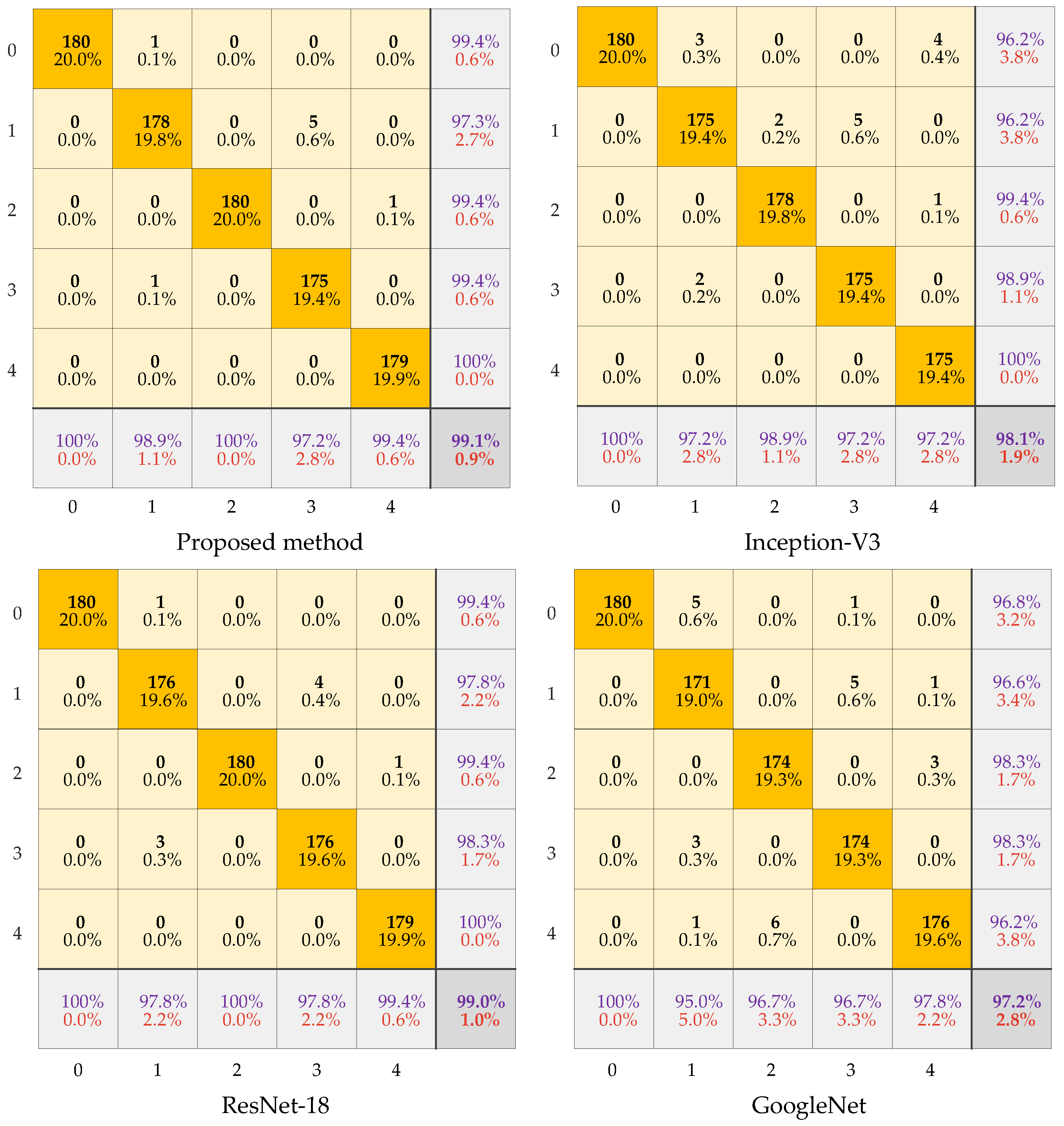
| Proposed method | 99.14% ± 0.0401 |
| Methods | Testing Accuracy | Training Time (s) |
|---|---|---|
| Proposed method (one PFRB) | 98.15% ± 0.1136 | 1954 |
| Proposed method (two PFRB) | 98.91% ± 0.1039 | 3018 |
| Proposed method (three PFRB) | 99.14% ± 0.0401 | 3780 |
| GoogleNet | 97.21% ± 0.0719 | 5982 |
| ResNet-18 | 99.08% ± 0.0724 | 5540 |
| Inception-V3 | 98.12% ± 0.0439 | 6078 |
Publisher’s Note: MDPI stays neutral with regard to jurisdictional claims in published maps and institutional affiliations. |
© 2022 by the authors. Licensee MDPI, Basel, Switzerland. This article is an open access article distributed under the terms and conditions of the Creative Commons Attribution (CC BY) license (https://creativecommons.org/licenses/by/4.0/).
Share and Cite
Meng, L.; Su, Y.; Kong, X.; Lan, X.; Li, Y.; Xu, T.; Ma, J. A Probabilistic Bayesian Parallel Deep Learning Framework for Wind Turbine Bearing Fault Diagnosis. Sensors 2022, 22, 7644. https://doi.org/10.3390/s22197644
Meng L, Su Y, Kong X, Lan X, Li Y, Xu T, Ma J. A Probabilistic Bayesian Parallel Deep Learning Framework for Wind Turbine Bearing Fault Diagnosis. Sensors. 2022; 22(19):7644. https://doi.org/10.3390/s22197644
Chicago/Turabian StyleMeng, Liang, Yuanhao Su, Xiaojia Kong, Xiaosheng Lan, Yunfeng Li, Tongle Xu, and Jinying Ma. 2022. "A Probabilistic Bayesian Parallel Deep Learning Framework for Wind Turbine Bearing Fault Diagnosis" Sensors 22, no. 19: 7644. https://doi.org/10.3390/s22197644
APA StyleMeng, L., Su, Y., Kong, X., Lan, X., Li, Y., Xu, T., & Ma, J. (2022). A Probabilistic Bayesian Parallel Deep Learning Framework for Wind Turbine Bearing Fault Diagnosis. Sensors, 22(19), 7644. https://doi.org/10.3390/s22197644