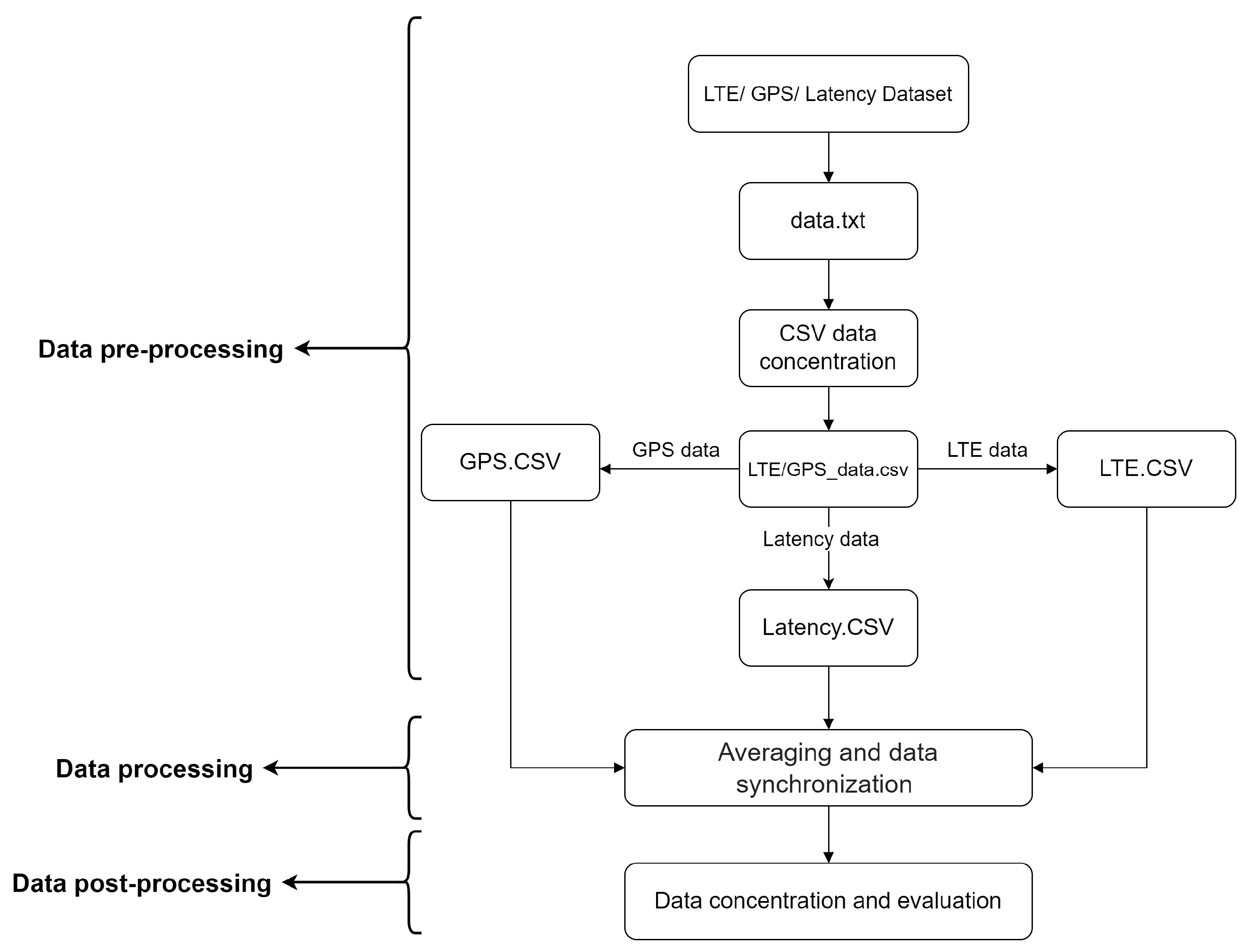
3.1.1. Positioning Data
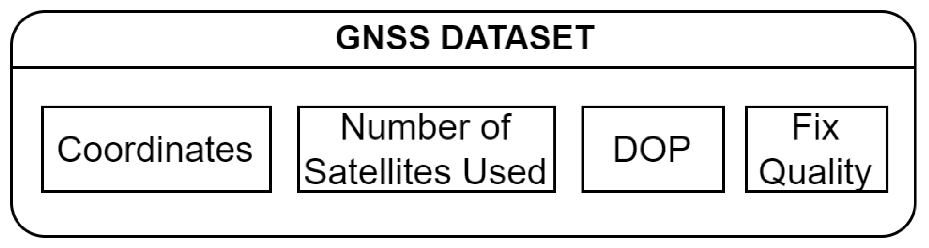
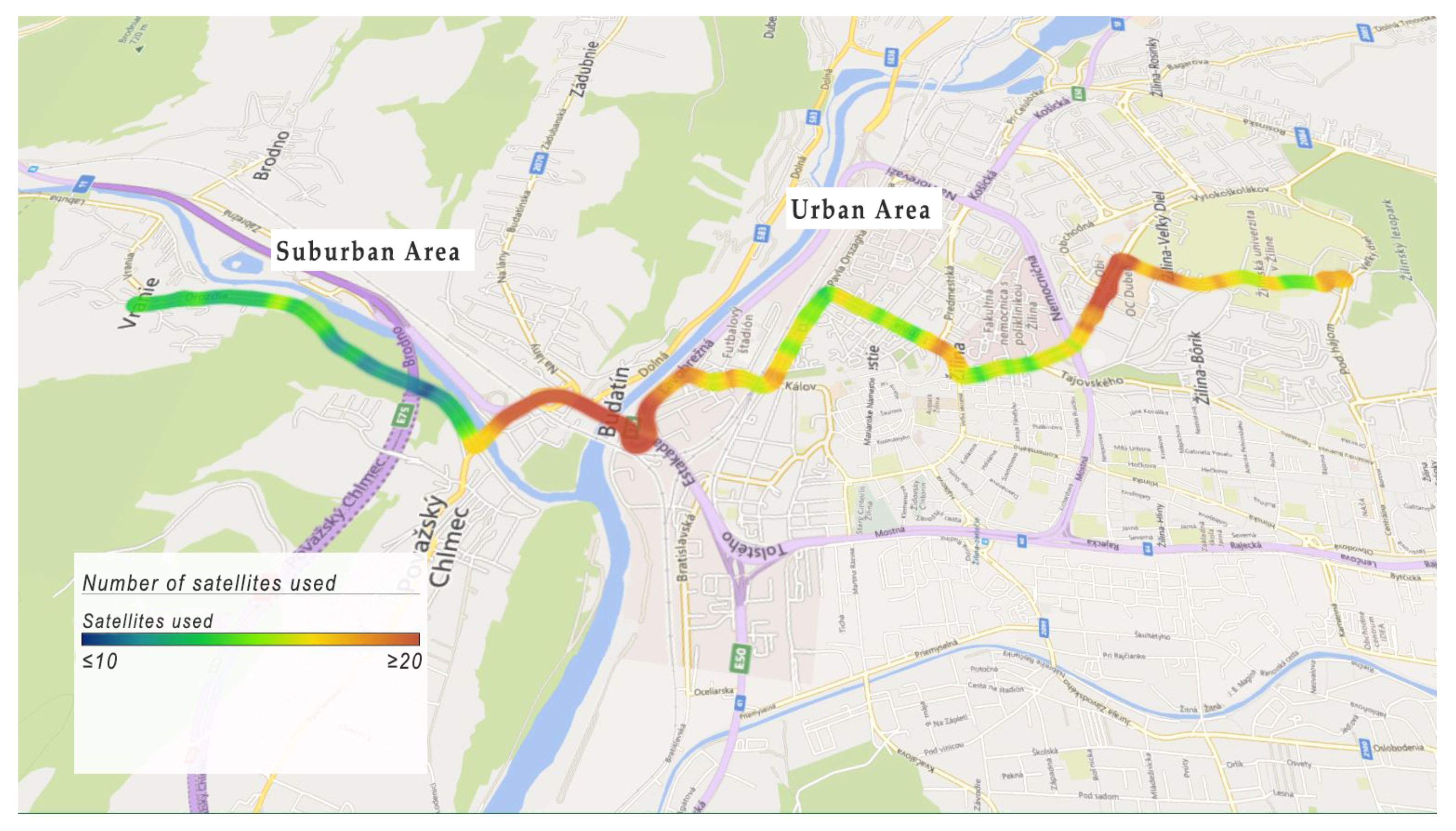
The used device supports GPS, GLONASS, BeiDou and Galileo GNSS standards. The following telemetry of GNSS was collected as is shown in
Figure 3—GPS coordinates, number of satellites used, Dilution of Precision (DOP) and fix quality.
The Dilution of Precision (DOP) is an important factor in determining positional errors in a GPS system. It is the collection of satellites’ geometry constellation from which signals are actually received. Basically, four satellites are the minimum required value to determine a complete positional fix in three dimensions. DOP is calculated using geometrical correlations between the position of the GPS receiver and the positions of the GPS satellites. The exact locations of these satellites relative to the receiver have an effect on the positional error. If the GPS receiver communicates with satellites spread throughout the sky, the calculated position will be more accurate, and the DOP value will be low. However, when satellites are close to each other, the calculated position will be less accurate, and the DOP value will be high [
34,
35]. In the following table, the DOP value rating is shown (
Table 6).
The following metrics are used to describe DOP. Position Dilution of Precision (PDOP), Horizontal Dilution of Precision (HDOP), Vertical Dilution of Precision (VDOP) and Time Dilution of Precision (TDOP).
PDOP describes the number of satellites used that are spread in the sky. The more satellites directly above GPS receiver are used, the lower the PDOP value is. The effect of DOP on the horizontal position is described by HDOP. The HDOP and horizontal position (latitude and longitude) are better when more GPS satellites are used. The effect of DOP on the vertical (altitude) position is referred to as VDOP. The time difference between the GPS satellites’ and the GPS receiver’s internal clocks are represented by TDOP. A low TDOP value represents more accurate time synchronization. Because DOP metrics are derived from convergence, they are not independent. For example, a high TDOP value represents worse clock synchronization, and it has an effect on positional error [
34,
36,
37].
The type of signal or technique used by the GPS receiver to establish its location is represented by the GPS fix status telemetry. The number of GPS satellites and techniques used by the GPS receiver are used to determine the GPS fix type technique. In general, the fix quality rating is given by numbers ranging from one to five, as
Table 7 shows. The fix quality number represents the type of GPS technique that was used to determine location. Each technique has a different accuracy. The used GPS technique can be GPSFix, Differential GPS (DGPS), Precise Positioning System (PPSFix), Fixed Real Time Kinematic (RTK Fixed) or Float Real Time Kinematic (RTK Float). The GPSFix describes a basic GPS technique or Standard Positioning Service (SPS). SPS is a standard service provided to any user worldwide, without qualification or restrictions. Based on US security interests, the accuracy of this service is determined by the US Department of Defense [
34,
37]. Unlike GPSFix, the DGPS technique utilizes a network of ground stations used to broadcast the divergence between indicated position by GPS satellites and the real known position. PPSFix stands for most precise localization technique provided by GPS. Only the Federal Government and military have access to this service, which is encrypted. The RTK Fixed technique is used to optimize position accuracy calculated by DGPS. The technique is based on carrier phase measurement of the GPS, GLONASS, Galileo. Thanks to high accuracy, this technique is used for geodetic measurement purposes. On the other hand, RTK Float is a similar technique as RTK Fixed but with low accuracy. The accuracy is decreased by skipping the phase initialization process, which increases the speed of position calculation [
34,
38,
39].
3.1.2. Connectivity Data
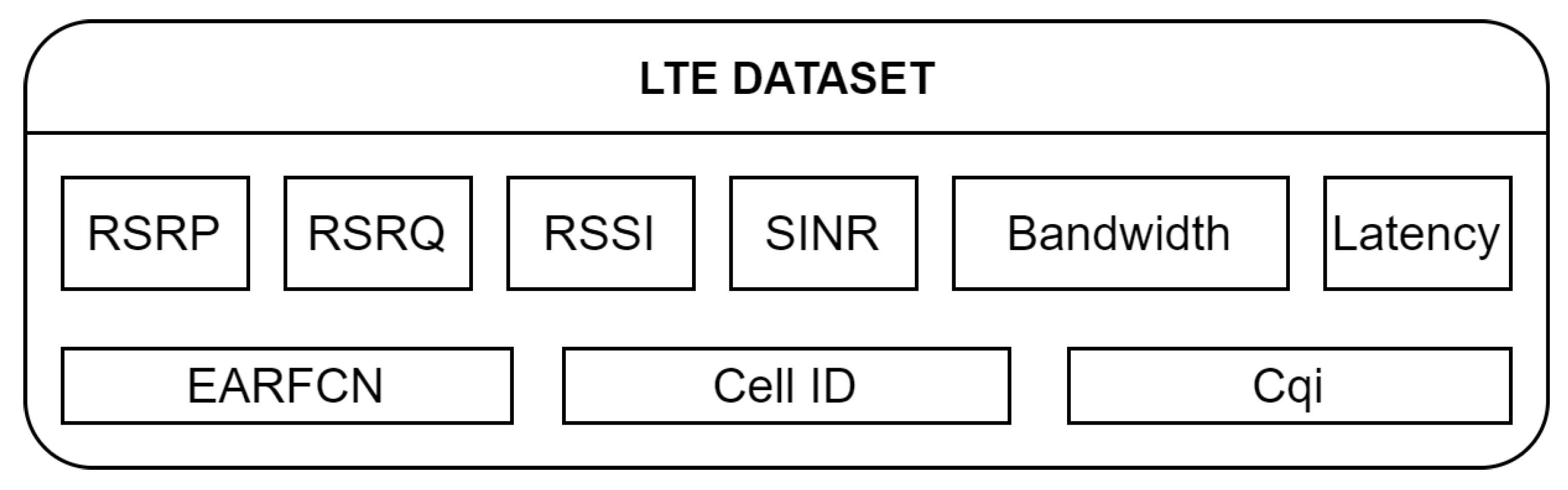
The following telemetry of LTE communication was collected, as is shown in
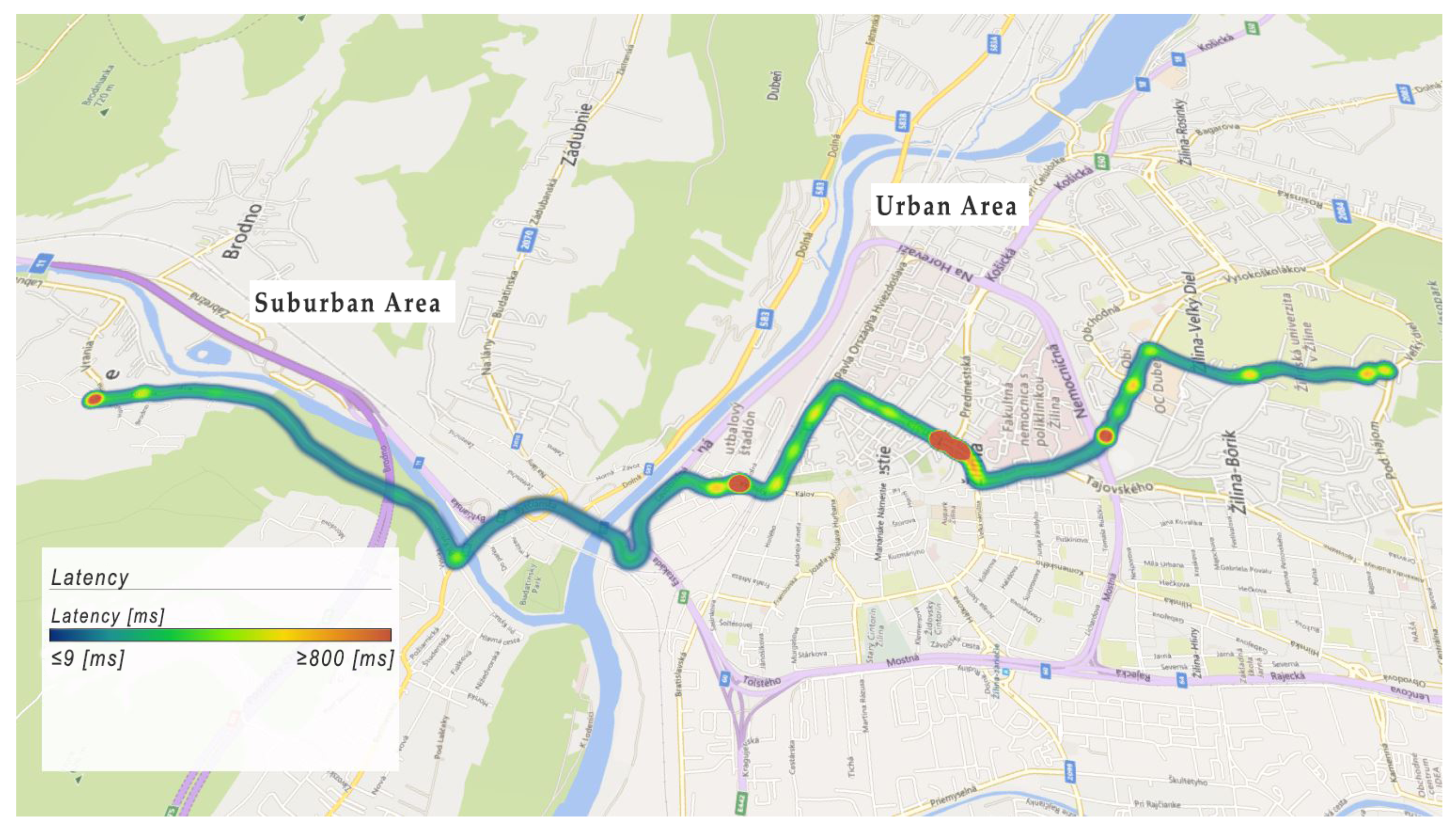
Figure 4. Communication latency, bandwidth, Signal Interference Noise Ratio (
SINR), Received Signal Strength Indicator (
RSSI), Reference Signal Received Quality (
RSRQ), Reference Signal Received Power (
RSRP), E-UTRA Absolute Radio Frequency Channel Number (
EARFCN), Cell Identification (Cell ID), Channel Quality Indicator (
CQI) and Rank Indicator (Ri).
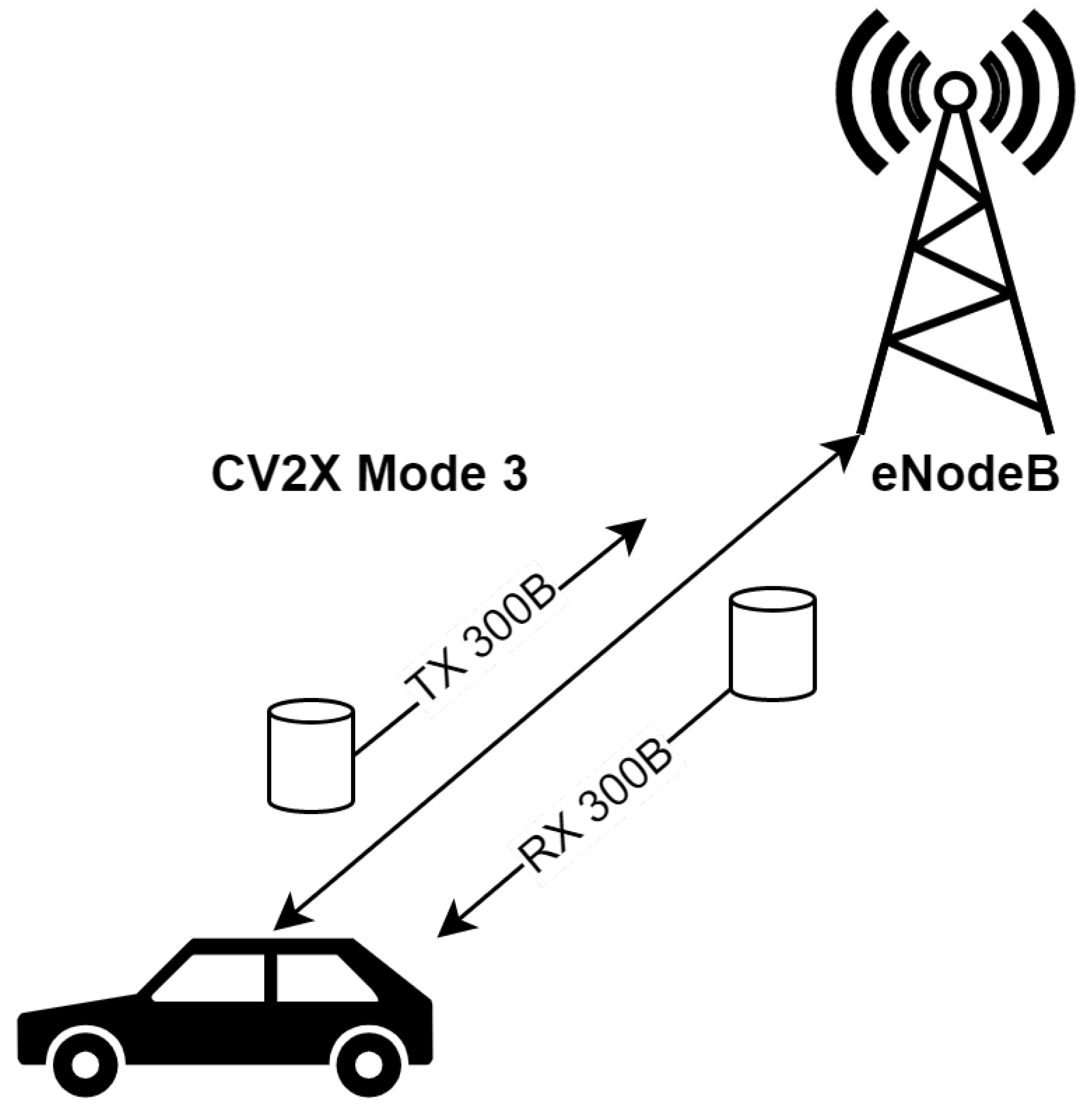
Our priority was to emulate the Cellular-V2X (C-V2X), as there is currently no DSRC- and VLC-enabled communication infrastructure available along the investigated route. We set up SBC to send communication packets periodically to a virtual server. We chose a packet length of 300 bytes and period of 100 ms since these values are commonly used to represent a transmission of CAM [
40]. The virtual server re-sent the packet back to SBC, as is shown in
Figure 5.
Each sent and received packet was marked with a time stamp by Network Time Protocol. The two-way latency communication
was calculated depending on packet transmit time
and packet received time
, as shown in equation:
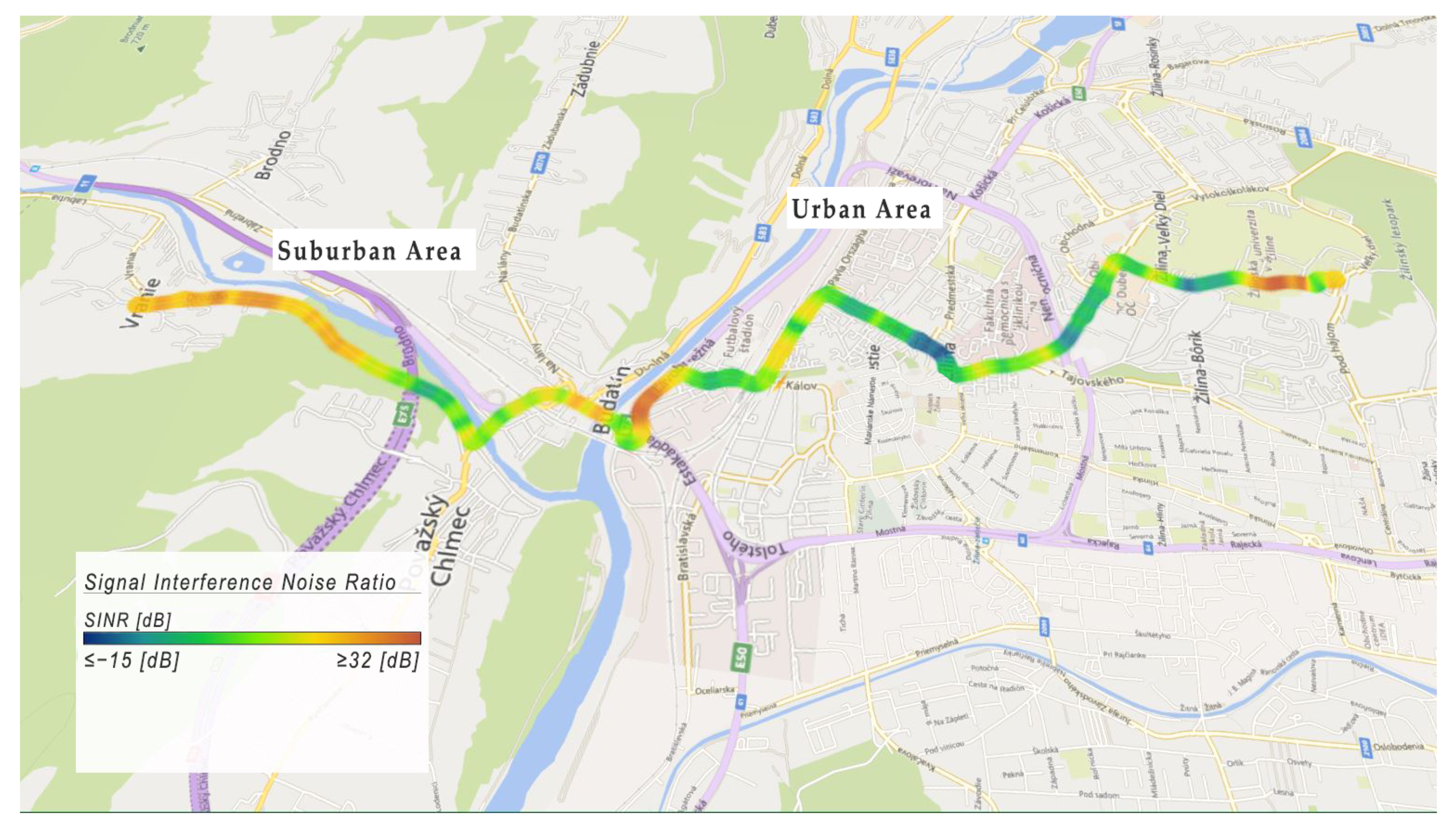
Signal Interference Noise Ratio (
SINR) represents the signal quality based on the strength of the wanted signal compared to the unwanted interference and noise. The
SINR is a metric used in cellular networks to determine if a particular frequency resource is acceptable for maintaining a communication link. The network employs
SINR to track radio link and handover failures. In systems that employ multiple access technologies based on frequency division, the scheduler can take
SINR into account while allocating frequency resources [
41]. It is a signal quality metric that is established by the User Equipment (UE) manufacturer instead of the 3GPP specifications. The basic
SINR mathematical expression is shown in Equation (
3):
where
S stands for the strength of the usable signals.
I stands for interference power of signals or channel interference signals from other cells.
N stands for background noise, which is proportional to measurement bandwidths and receiver noise coefficients.
Table 8 shows the standard
SINR values and signal quality category.
Higher
SINR values can affect the spectral efficiency as it enables the receiver to decode a higher Modulation Coding Scheme (MCS). To provide the best possible User Experience, the network operator attempts to optimize
SINR at all locations, either by transmitting at a greater power or by avoiding interference and noise [
43].
SINR optimization can aid in achieving higher cell capacity by allowing higher QAM modulation, which results in greater peak data rates, fewer missed calls, and an overall better quality of user experience [
44].
Received Signal Strength Indicator (
RSSI) is an LTE metric that states how much overall wideband power measured in symbols have been received, including all interference and thermal noise. UE does not send
RSSI values to eNodeB. It may be easily calculated using
RSRQ and
RSRP, which are instead reported by UE. The value is measured in dBm.
RSSI is defined as [
45]:
where
S,
I and
N are the same parameters as in the
SINR equation.
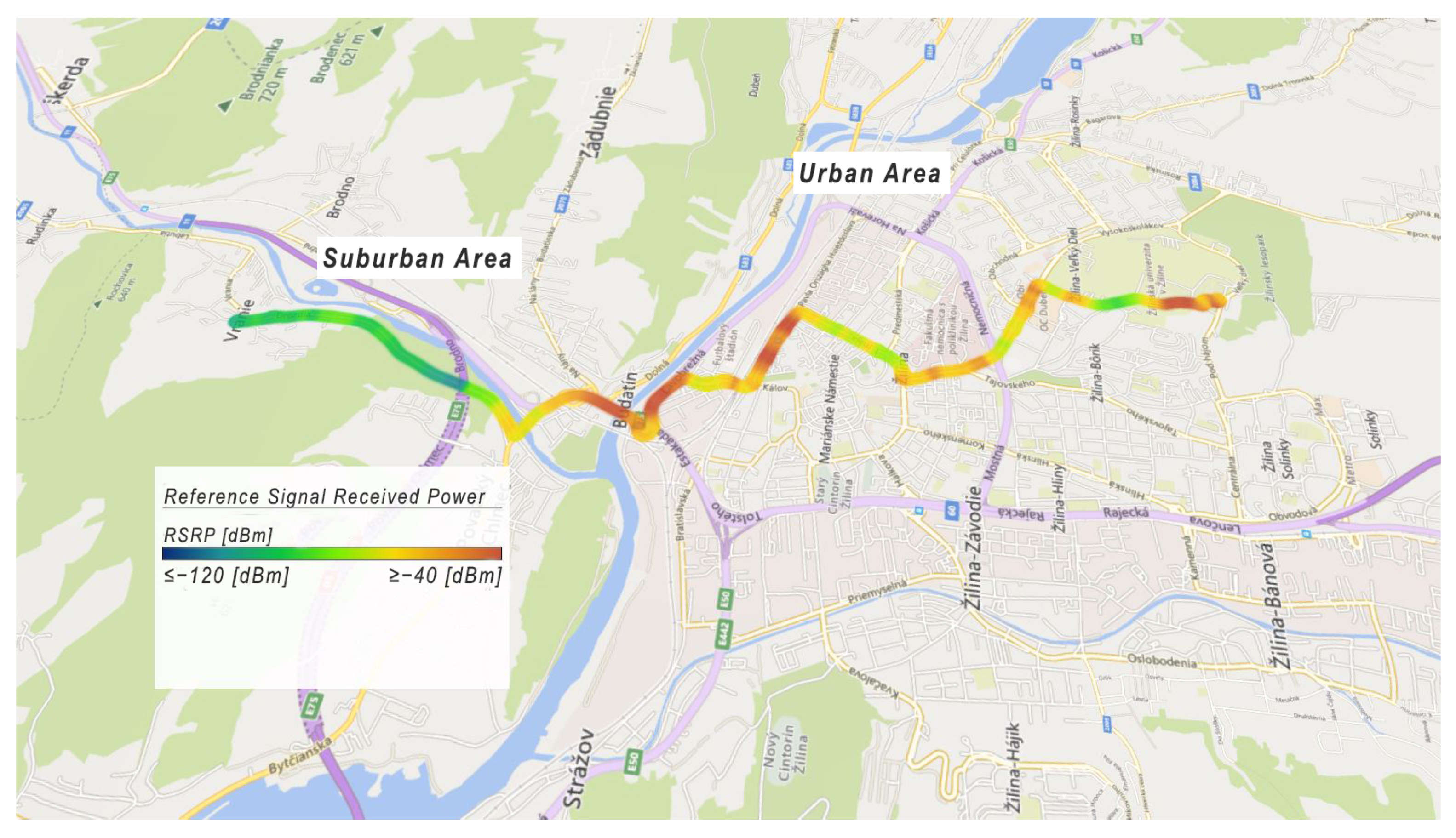
Reference Signal Received Power (
RSRP) and Refence Signal Received Quality (
RSRQ) are two main key signal level and quality indicators for current LTE networks. When a UE goes from cell to cell in a cellular network and conducts handover, it performs a measurement of the reference signal strength and quality of serving and neighbor cells for successful execution of the handover process. In essence, it is the power of the received signal from eNodeB by UE [
42]. Based on
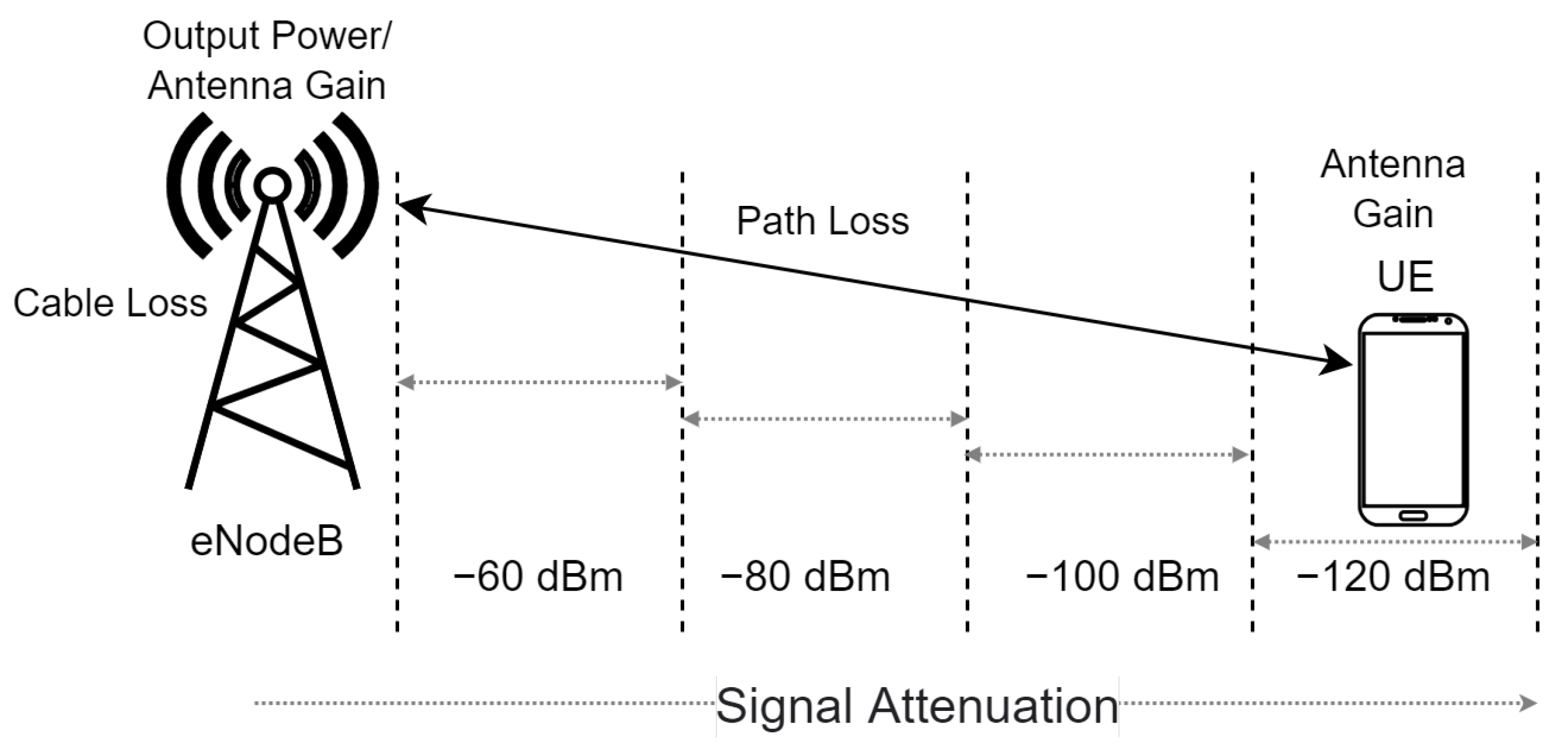
RSRP, it is possible to compare the strengths of signals from individual cells in LTE networks. The measurement process is shown in
Figure 6.
Figure 6 shows eNodeB and UE, which receive the reference signal from the eNodeB. The closer the UE is to the eNodeB location, the stronger the received signal. The reporting range of
RSRP is defined from −140 to −44 dBm with 1 dB resolution [
42].
Table 9 shows the standard
RSRP values and signal quality category.
The
RSRP calculation is shown in Equation (
5), where
N stands for Number of PRBs (Physical Resource Blocks) [
42,
47,
48].
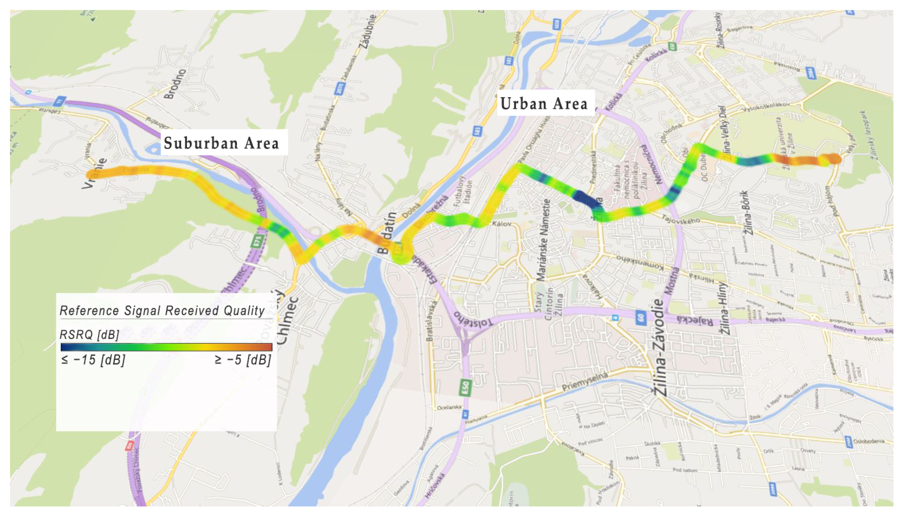
RSRQ telemetry parameter is the proportion of
RSRP to wideband power.
RSRQ represents signal quality received by the UE. The signal, noise, and interference received by the UE also have an effect on the
RSRQ [
40,
42]. The following equation [
42] is used for
RSRQ calculation, where
N stands for Number of Physical Resource Blocks (PRBs).
The reporting range of
RSRQ is defined from −3 to −20 dB.
Table 10 shows the standard
RSRQ values and signal quality category.
Instead of reporting raw carrier frequencies in MHz, LTE base stations use the ETSI E-UTRA Absolute Radio Frequency Channel Number (EARFCN) industry standard to report channel numbers. In LTE technology, EARFCN determines the carrier frequency in the uplink and downlink, the range of which is from 0 to 65,535. The equations below express the relationship between EARFCN and its uplink/downlink carrier frequency [
49].
where
NDL stands for downlink EARFCN,
NUL for uplink EARFCN,
Noffs-UL offset used to calculate uplink EARFCN,
Noffs-DL offset used to calculate downlink EARFCN. The values
FUL-low,
FDL-low,
NDL,
NUL,
Noffs-DL,
Noffs-UL are given in [
49] by ETSI.
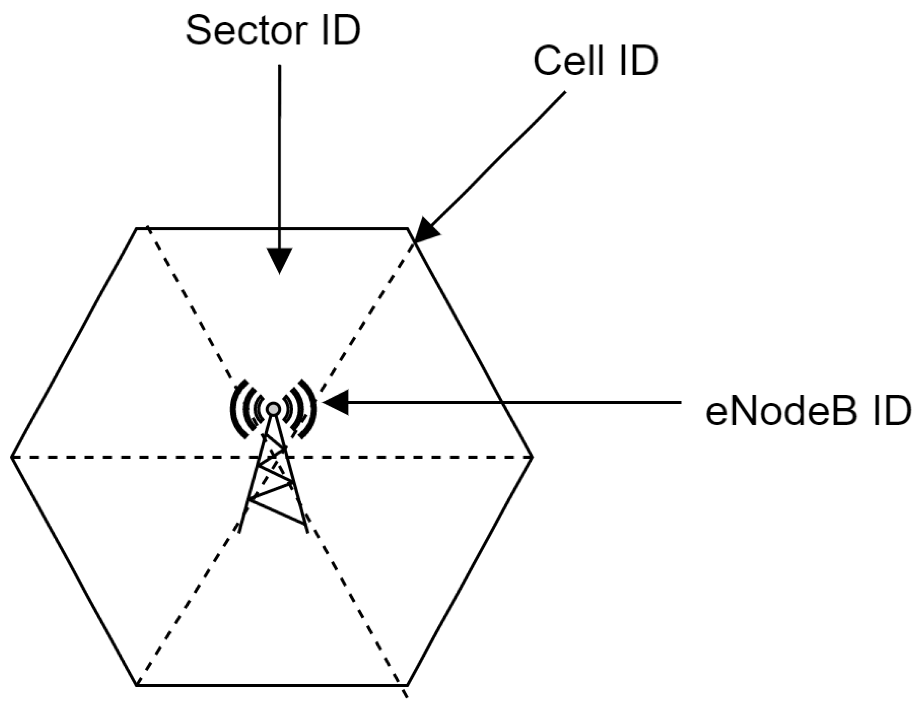
For unique identification of LTE components, the identification numbers are used. As shown in
Figure 7, we have three main key identifiers in the LTE cell. The E-UTRAN Cell Identifier (ECI) represents the identity of a cell within a Public Land Mobile Network Identifier (PLMN). ECI consists of 28 bits where the first 20 bits represent the eNodeB ID number and the last 8 bits are stated for cell ID. The sector ID identifies a particular antenna in cell sectors [
50,
51].
The code rate and modulation are defined by MCS in the LTE. MCS specifies the maximum number of usable bits that can be transferred per Resource Element (RE), and it is affected by radio channel quality.
Table 11 shows the CQI-MCS mapping for LTE rel. 12 and beyond. The better channel quality is represented by a higher MCS, and the more useful data can be transmitted. In other words, MCS depends on error probability. In LTE, a Turbo encoder with a 1/3 coding rate is employed. The actual ratio of usable bits to total transmitted bits (useful bits + parity bits) is dependent on the quality of the radio link. The range of coding rates is 0.0762 to 0.9258.
Radio link quality is estimated based on the Channel Quality Indicator (
CQI). The
CQI parameter is reported by UE to the eNodeB. The
CQI measurement is based on the Cell Reference Signal (CRS) [
52]. Better radio condition is represented by higher
CQI and the higher coding rate, as is shown in the table below. Bits per RE column should be multiplied by the number of data streams to obtain a final value in case of MIMO usage [
52].
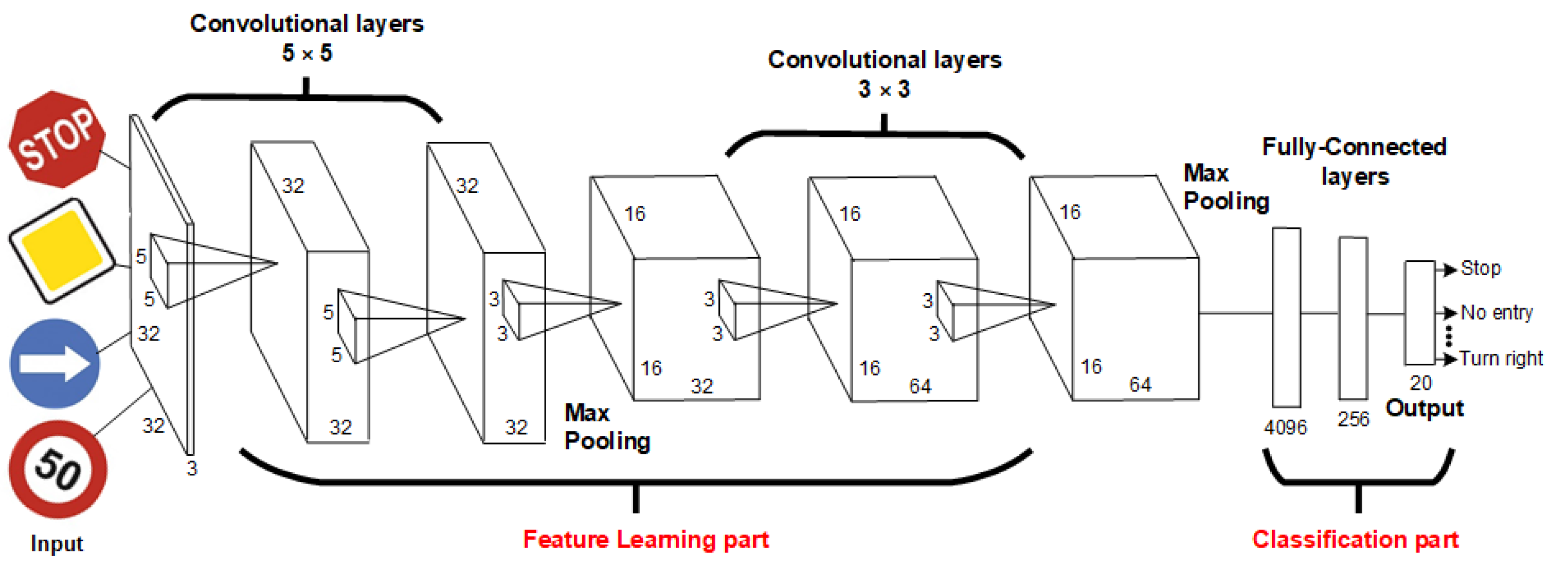
3.1.3. Collection of Image Data
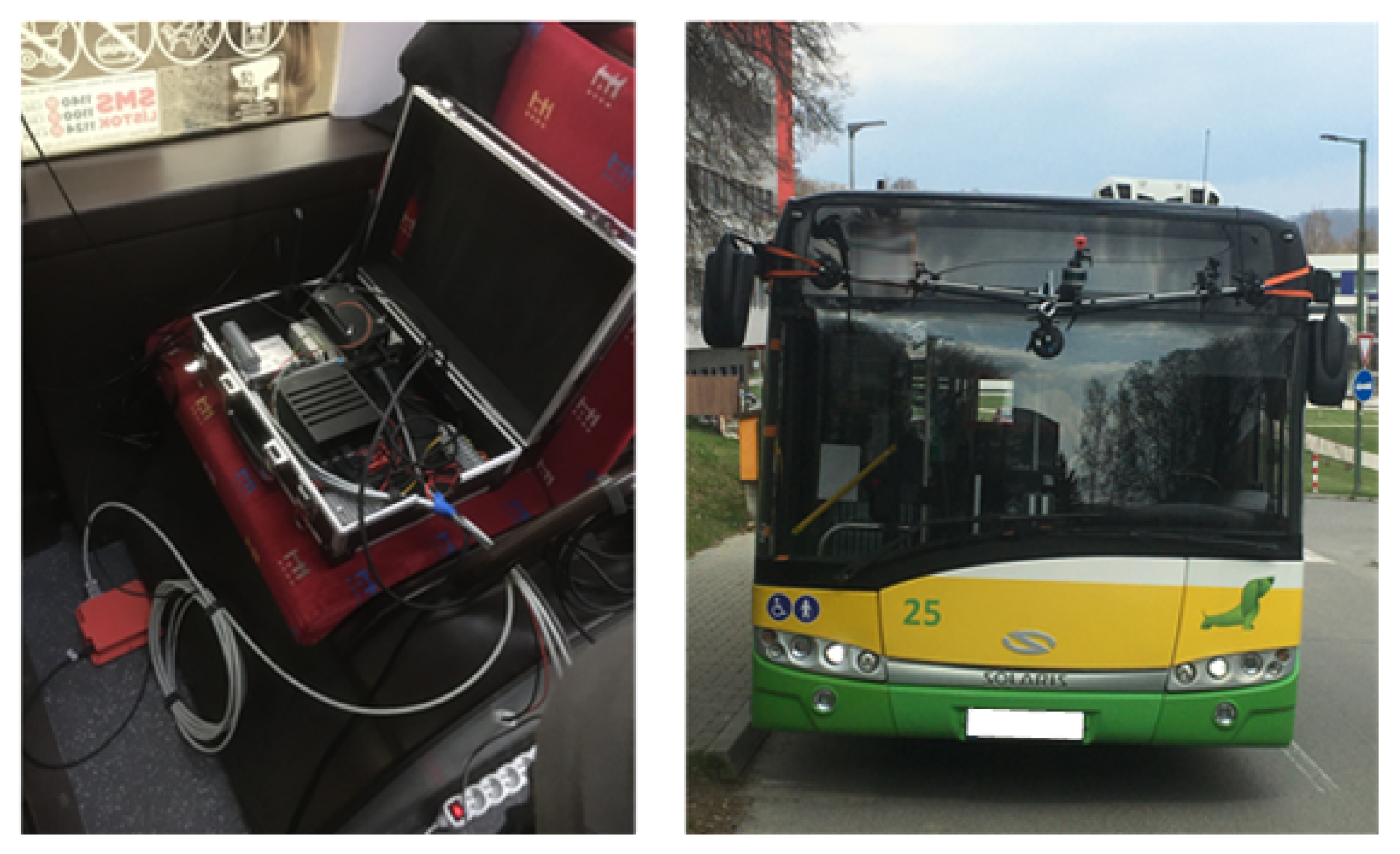
For image data collection, the OmniVision OV10640 camera system (OmniVision, Santa Clara, CA, USA) was used. This sensor uses a proprietary technology, which delivers an image with a very high dynamic range (HDR). Furthermore, the sensor is encapsulated in a compact package, which can be easily deployed for a wide range of automotive applications (see
Table 12). A total of four cameras were used on the bus (one on the windshield recorded the area in front of the bus, one on the rear window recorded the area behind the bus, and one on each side recorded the area on the sides of the bus).
Three cameras were used in the collection of image data. Two cameras were placed on the sides of the bus and one in the middle of the bus above the windshield (see
Figure 8). The cameras located on the sides of the bus had a standard horizontal field of view (52 degrees). The middle camera capturing objects in front of the bus was a fisheye (horizontal field of view of 194 degrees).
Furthermore, the sensor is capable of sampling the recorded scene simultaneously instead of sequentially, which helps to minimize the distortion caused by motion.
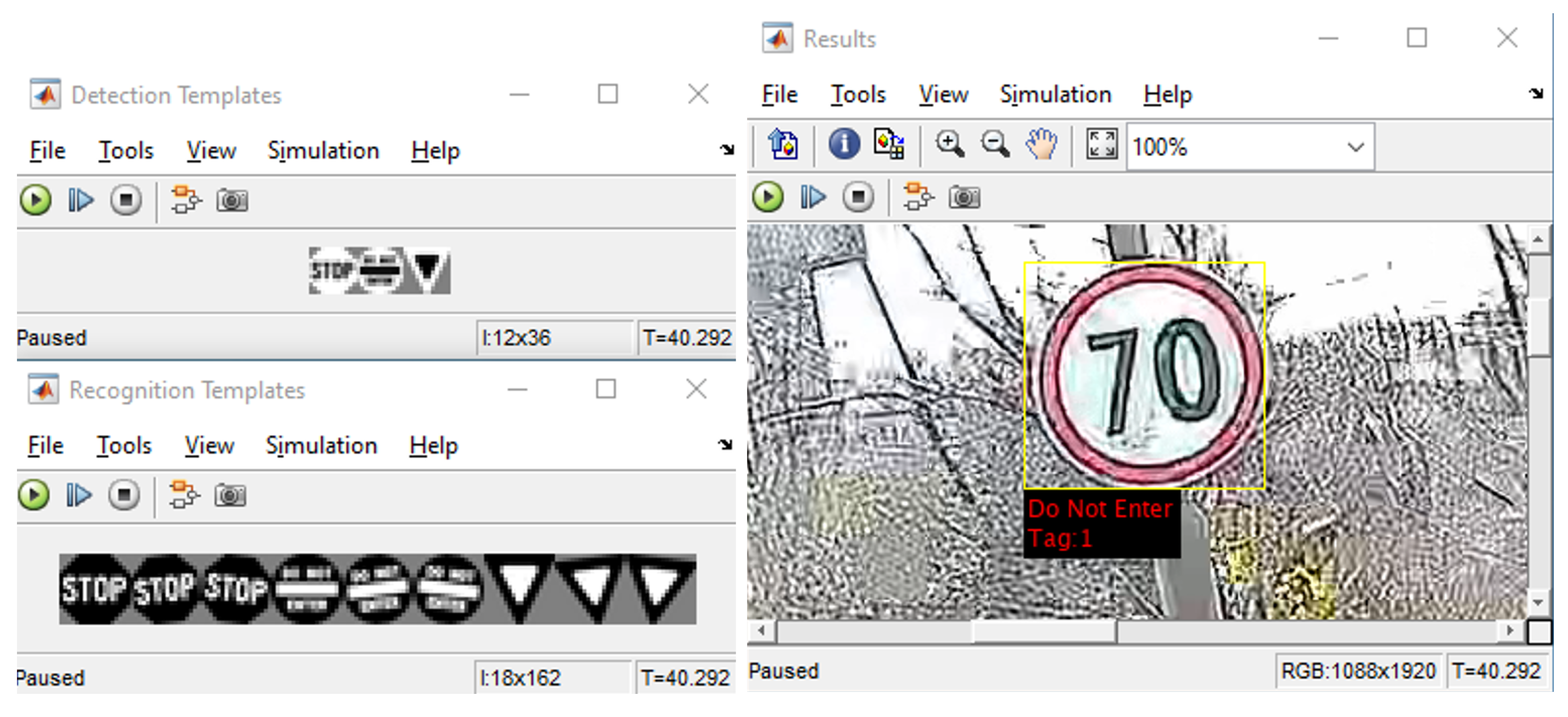
The image dataset contains classes representing traffic signs and also classes representing road users, as is shown in
Figure 9.
Table 13 shows all the classes that our image dataset contains. The first column contains the number of classes, and the second column shows the specification of the given class.


