

_Sun.png)
Hierarchical Dynamic Bayesian Network-Based Fatigue Crack Propagation Modeling Considering Initial Defects


Abstract
:1. Introduction
2. Hierarchical Dynamic Bayesian Network for Fatigue Crack Propagation (FCP)
2.1. Fracture Mechanics-Based Multi-Source Uncertainty Analysis
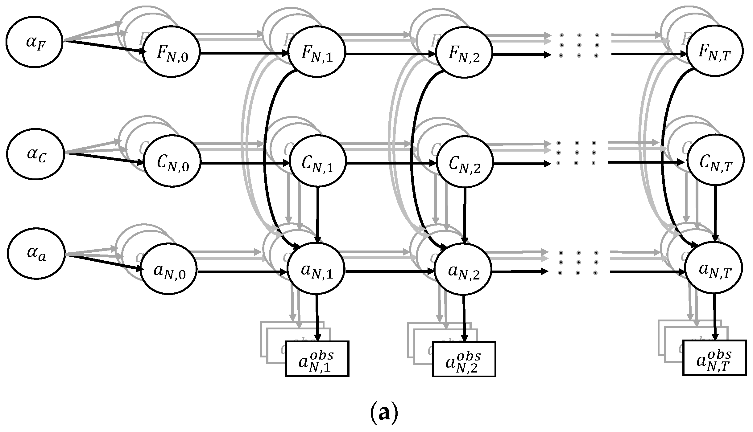
2.2. Hierarchical Dynamic Bayesian Network for FCP of OSD System
2.3. Refined Exact Inference Algorithm for Dynamic Bayesian Network Updating
3. Implementation Details
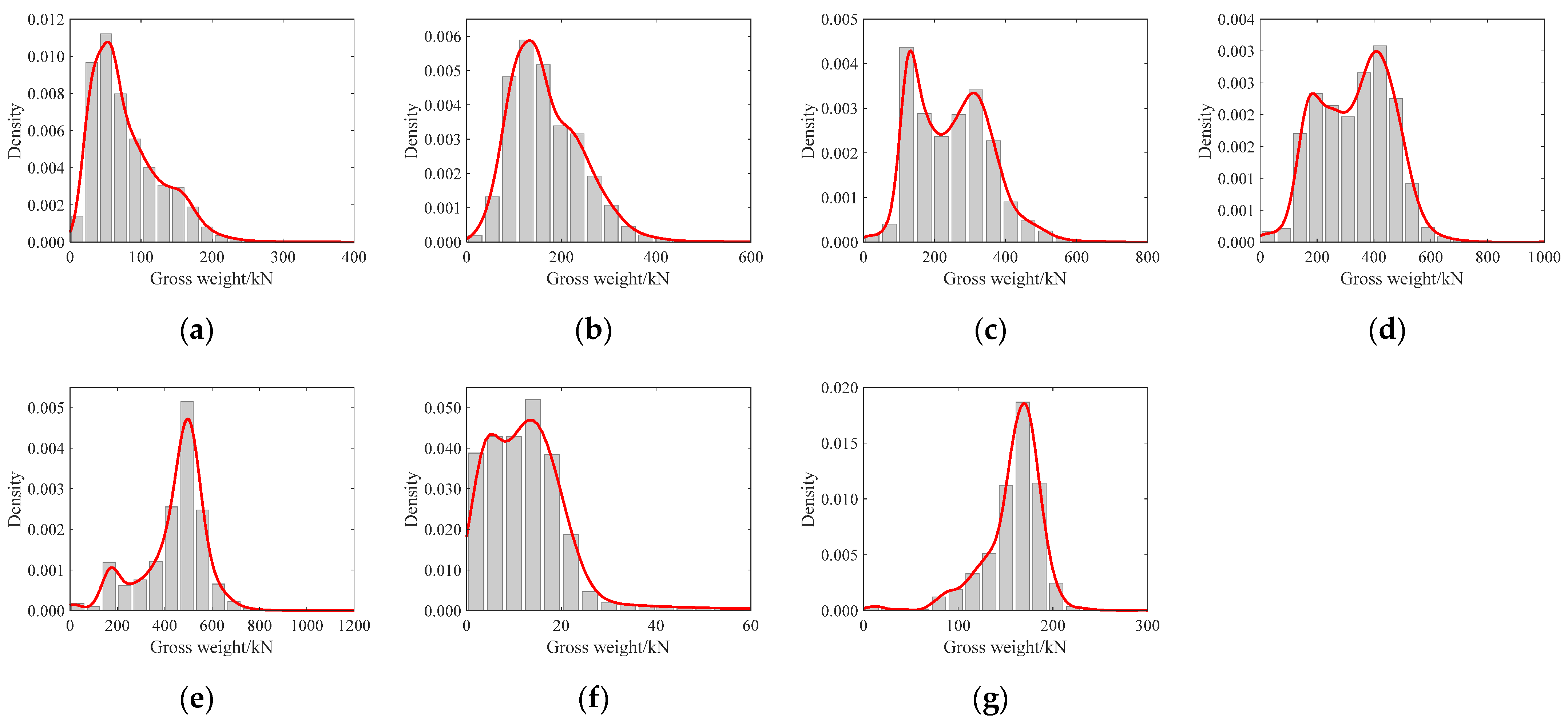
3.1. Stochastic Traffic Flow Model
3.2. Multi-Scale Finite Element Analysis
3.3. Parameter Setups in Hierarchical DBN for FCP Analysis
4. Results and Discussion
4.1. Demonstration by Numerical Simulations
- (1)
- (2)
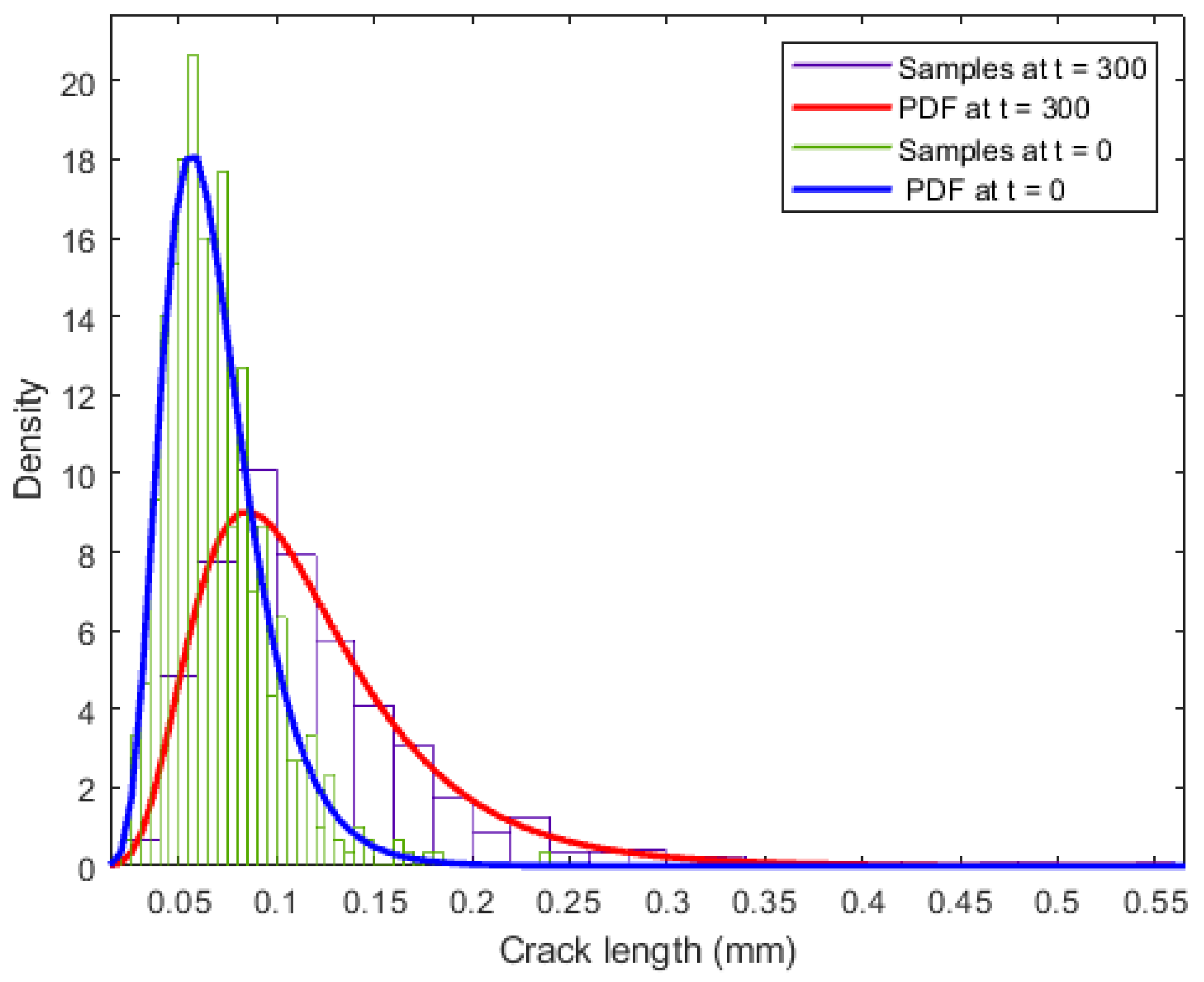
- For each combination of , FCP analysis is performed in a continuous space based on Equation (6). The comparison of the probability distribution of crack length at t = 0 and t = 300 is shown in Figure 11, which indicates a significant increase in crack length.
- (3)
- Then, crack lengths under each combination at time steps t = 300:10:390 are predicted and transferred into the discrete states based on the discretization scheme shown in Table 1.
- (4)
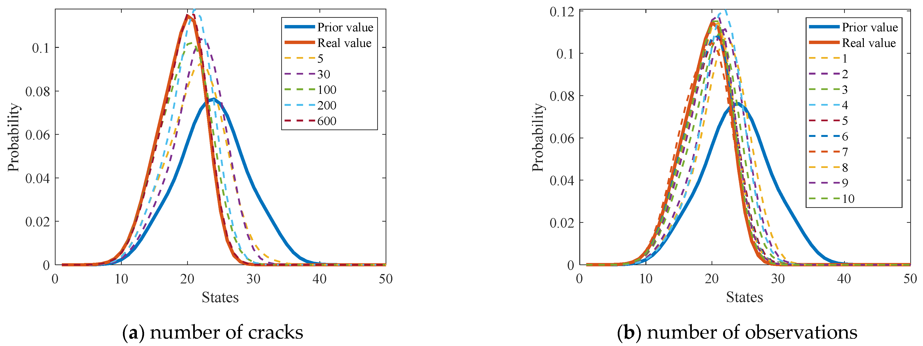
- The simulated states of different cracks at time steps t = 300:10:390 are utilized to update the prior probability distribution of parent-node hyperparameters and the EICS using the refined exact inference algorithm introduced in Section 2.3.

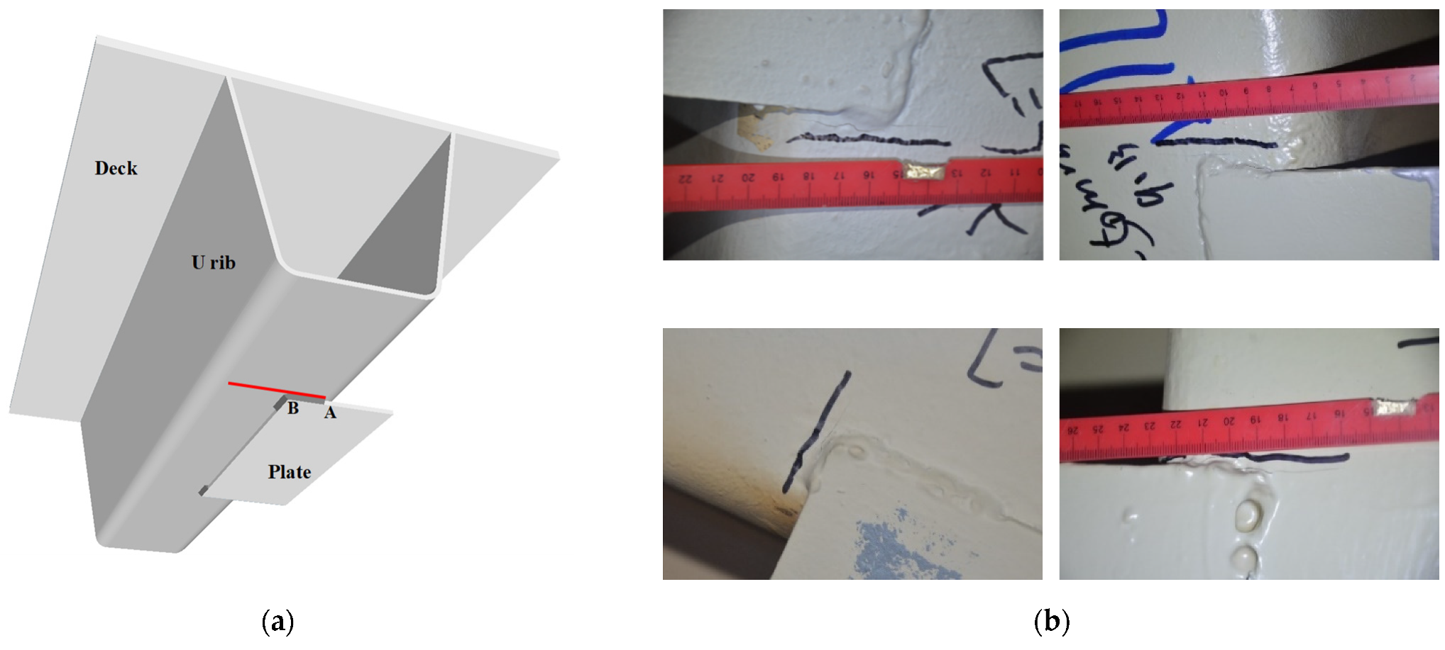
4.2. Demonstration by Actual Bridge Inspections
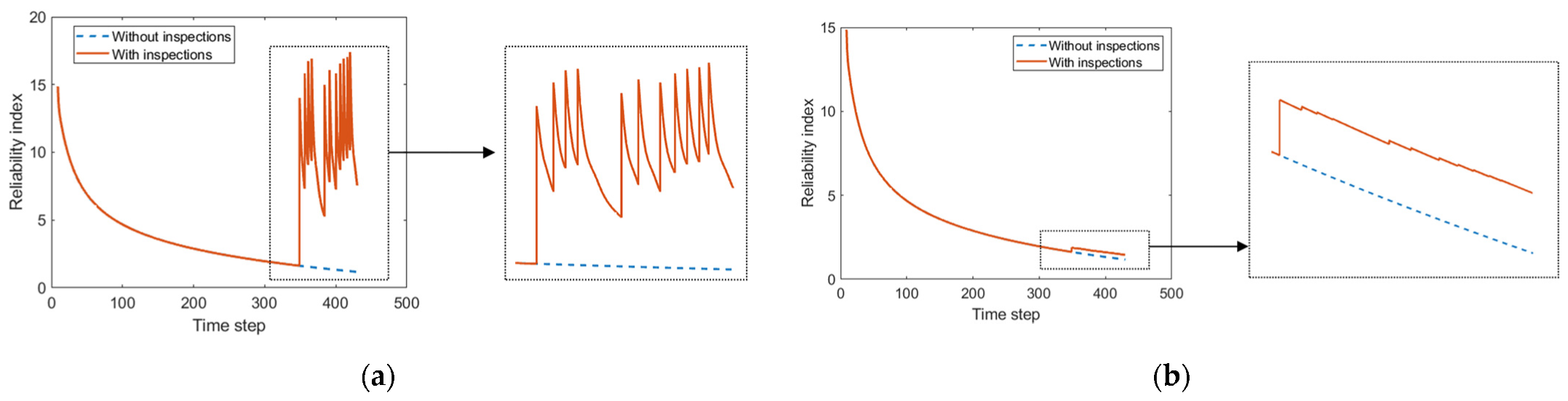
4.3. Prediction of Component-Level Fatigue Reliability
5. Conclusions
- (1)
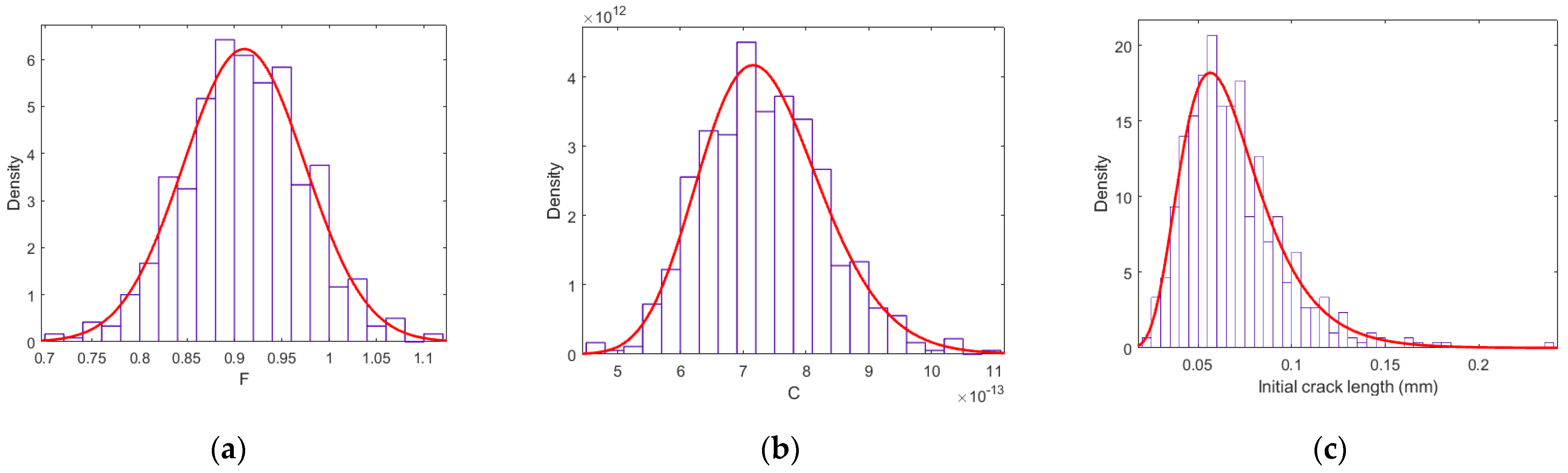
- Fracture mechanics-based uncertainty analysis is performed to determine uncertainty sources in the Paris crack propagation model, material property, and observation data of crack length. The uncertainty of monitoring data of vehicle loads is ignored because of the high accuracy of the WIM system. Actual applications also demonstrate that the vehicle-load-related uncertainty can be ignored.
- (2)
- A hierarchical DBN model is introduced to construct mutual dependences and correlations among various uncertainties for fatigue crack propagation in different components. A refined exact inference algorithm is adopted to estimate the posterior distribution of EICS and update the DBN model in a forward–backward–forward manner. In addition, the component-level reliability index can be updated.
- (3)
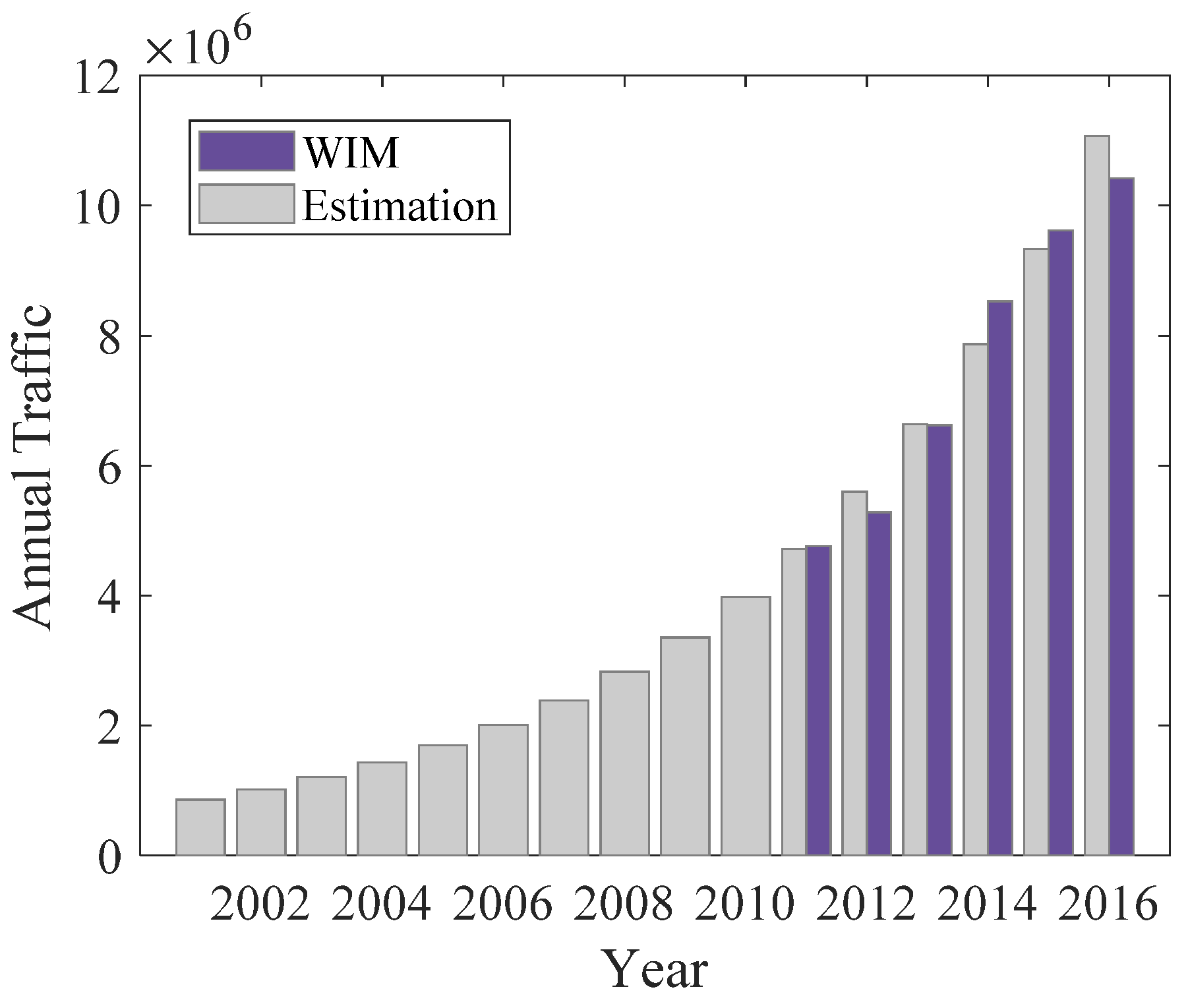
- A stochastic traffic model is established using the WIM monitoring data and multi-scale finite element analysis via substructure techniques. Numerical case studies and actual bridge inspections are performed to validate the effectiveness of the established hierarchical DBN model for FCP analysis.
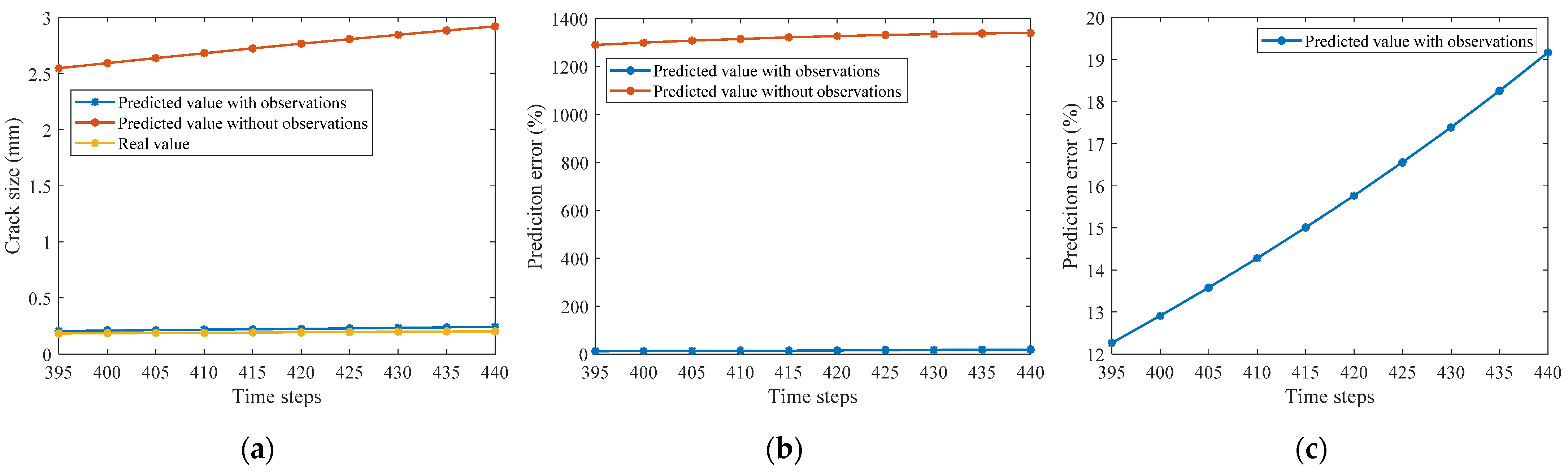
- (4)
- The results show that the established DBN model is robust to random observation errors and that the current and future states of the concerned fatigue crack can be updated by the observation data of other cracks based on the hierarchical DBN model, indicating that the proposed method constructs the dependencies and correlations among different fatigue cracks well.
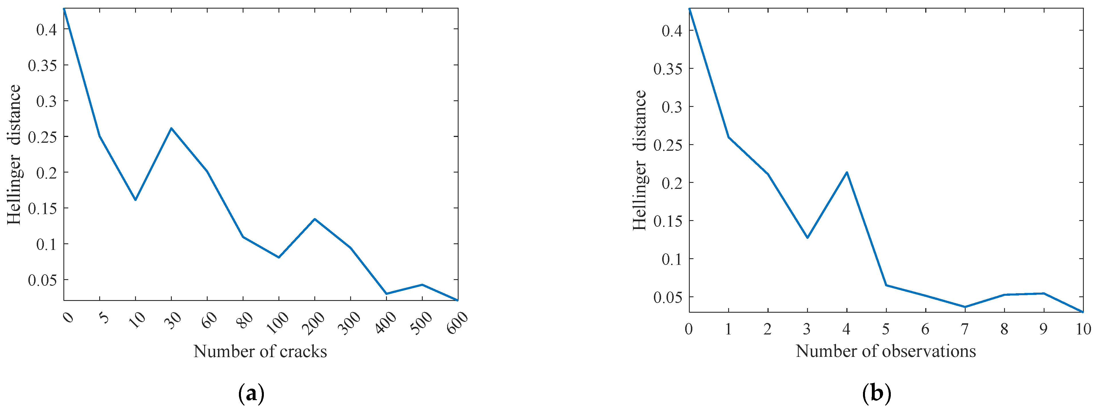
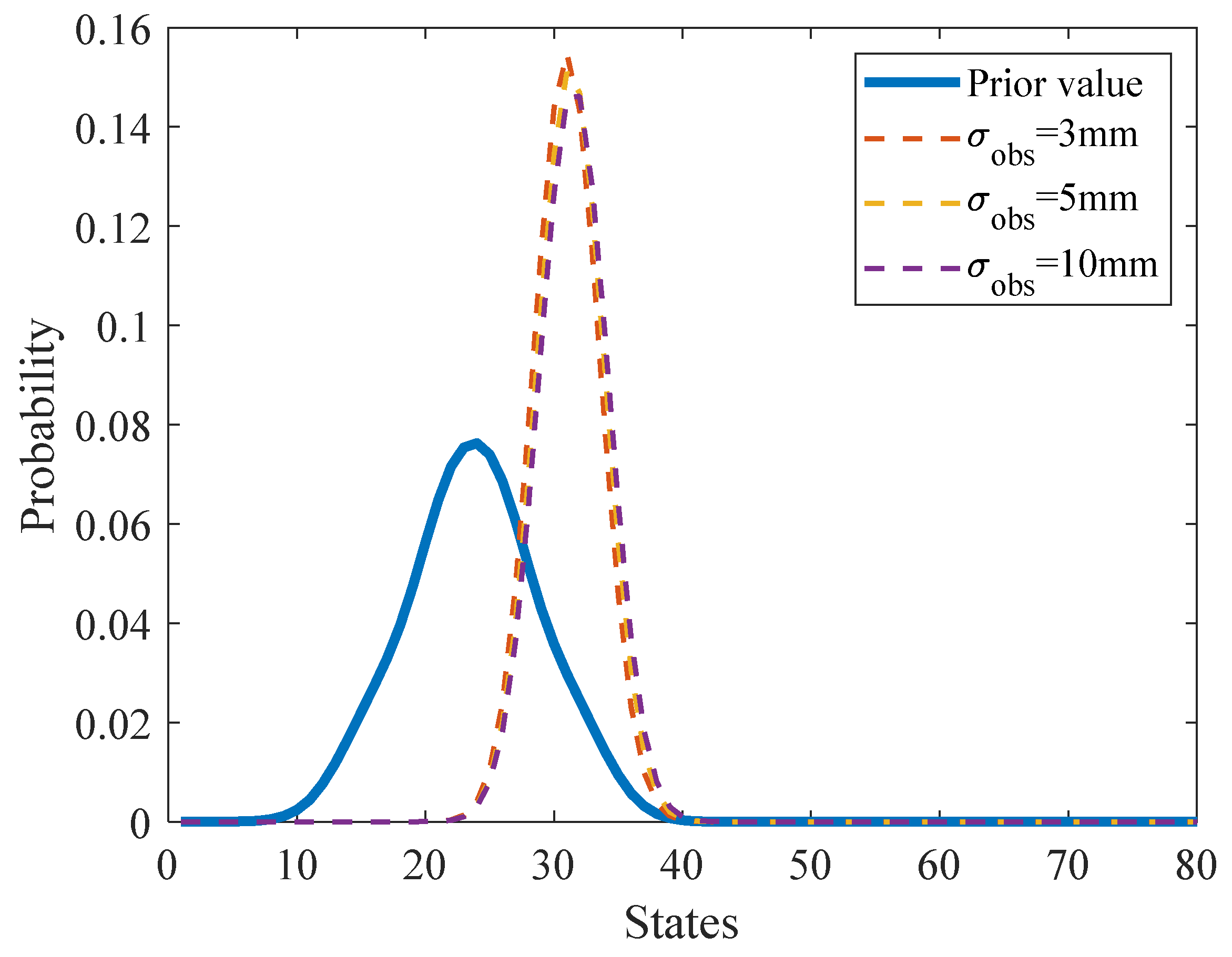
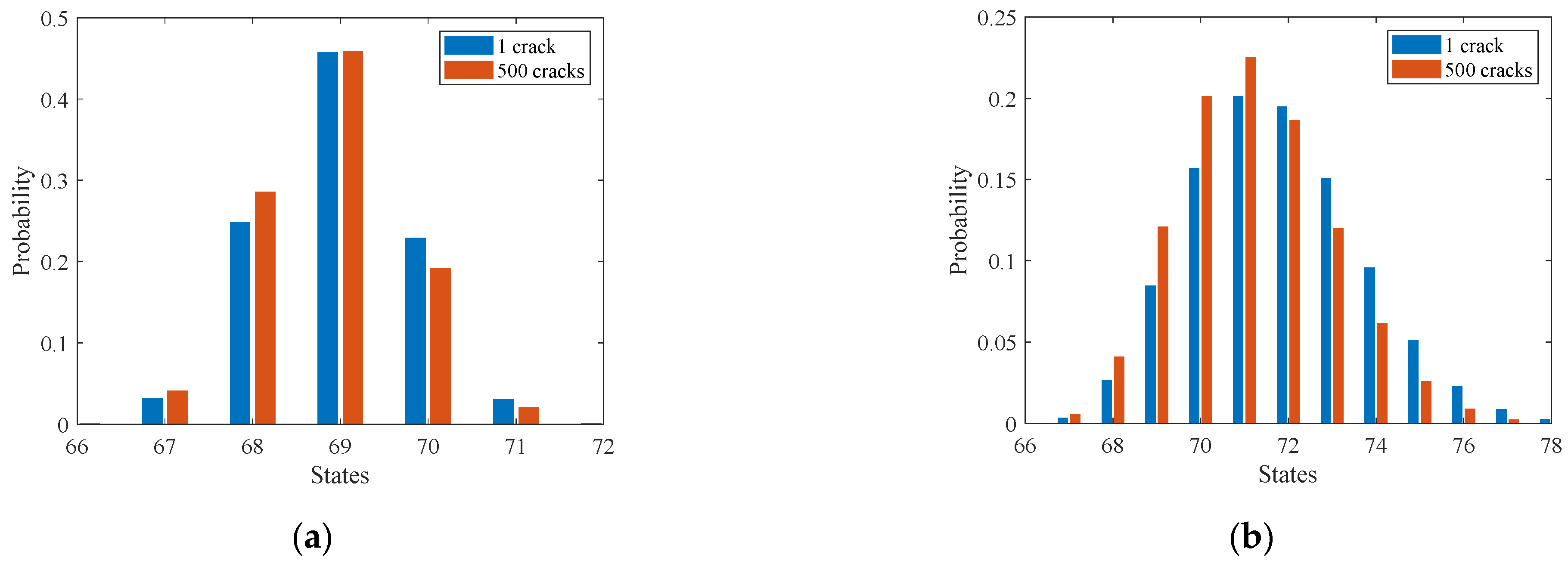
- (5)
- Numerical experiments demonstrate that using more temporal–spatial inspection data leads to a much more precise estimation of the probability distribution of the initial crack size. It also demonstrates that considering the observation uncertainty of crack length enables the accurate estimation of the probability distribution for EICS. The predictability of the proposed method on fatigue crack propagation forecast is also verified.
Author Contributions
Funding
Institutional Review Board Statement
Informed Consent Statement
Data Availability Statement
Acknowledgments
Conflicts of Interest
References
- Paris, P.; Erdogan, F. A critical analysis of crack propagation laws. J. Basic Eng. 1963, 85, 528–533. [Google Scholar] [CrossRef]
- Ayala-Uraga, E.; Moan, T. Reliability based assessment of welded joints using alternative fatigue failure functions. In Proceedings of the International Conference on Structural Safety and Reliability ICOSSAR, Rome, Italy, 19–23 June 2005. [Google Scholar]
- Moan, T. Reliability-based management of inspection, maintenance and repair of offshore structures. Struct. Infrastruct. Eng. 2005, 1, 33–62. [Google Scholar] [CrossRef]
- Ayala-Uraga, E.; Moan, T. Fatigue reliability-based assessment of welded joints applying consistent fracture mechanics formulations. Int. J. Fatigue 2007, 29, 444–456. [Google Scholar] [CrossRef]
- Wang, Y.; Sun, Y.; Lv, P.; Wang, H. Detection of line weld defects based on multiple thresholds and support vector machine. NDT E Int. 2008, 41, 517–524. [Google Scholar]
- Yang, D.Y.; Frangopol, D.M. Evidence-based framework for real-time life-cycle management of fatigue-critical details of structures. Struct. Infrastruct. Eng. 2018, 14, 509–522. [Google Scholar] [CrossRef]
- Cui, C.; Zhang, Q.; Bao, Y.; Bu, Y.; Luo, Y. Fatigue life evaluation of welded joints in steel bridge considering residual stress. J. Construct. Steel Res. 2019, 153, 509–518. [Google Scholar] [CrossRef]
- Bokalrud, T.; Karlsen, A. Probabilistic fracture mechanics evaluation of fatigue failure from weld defects in butt welded joints. In Proceedings of the Conference on Fitness for Purpose Validation of Welded Constructions, London, UK, 17–19 November 1981. Paper 28. [Google Scholar]
- Moan, T.; Vårdal, O.T.; Hellevig, N.C.; Skjoldli, K. Initial crack depth and POD values inferred from in-service observations of cracks in North Sea jackets. J. Offshore Mech. Arct. Eng. 2000, 122, 157–162. [Google Scholar] [CrossRef]
- Lee, D.; Achenbach, J.D. Analysis of the reliability of a jet engine compressor rotor blade containing a fatigue crack. J. Appl. Mech. 2016, 83, 041004. [Google Scholar] [CrossRef]
- Cui, C.; Zhang, Q.; Luo, Y.; Hao, H.; Li, J. Fatigue reliability evaluation of deck-to-rib welded joints in OSD considering stochastic traffic load and welding residual stress. Int. J. Fatigue 2018, 111, 151–160. [Google Scholar] [CrossRef]
- Murphy, K.P. Dynamic Bayesian Networks: Representation, Inference and Learning; University of California: Berkeley, CA, USA, 2002. [Google Scholar]
- Koski, T.; Noble, J. Bayesian Networks: An Introduction; John Wiley & Sons: Hoboken, NJ, USA, 2011. [Google Scholar]
- Straub, D. Stochastic modeling of deterioration processes through dynamic Bayesian networks. J. Eng. Mech. 2009, 135, 1089–1099. [Google Scholar] [CrossRef]
- Zhu, J.; Collette, M. A dynamic discretization method for reliability inference in Dynamic Bayesian Networks. Reliab. Eng. Syst. Saf. 2015, 138, 242–252. [Google Scholar] [CrossRef]
- Li, C.; Mahadevan, S.; Ling, Y.; Choze, S.; Wang, L. Dynamic Bayesian network for aircraft wing health monitoring digital twin. AIAA J. 2017, 55, 930–941. [Google Scholar] [CrossRef]
- Chen, L.; Arzaghi, E.; Abaei, M.M.; Garaniya, V.; Abbassi, R. Condition monitoring of subsea pipelines considering stress observation and structural deterioration. J. Loss Prev. Process Ind. 2018, 51, 178–185. [Google Scholar] [CrossRef]
- Maes, M.A.; Dann, M. Hierarchical Bayes methods for systems with spatially varying condition states. Can. J. Civ. Eng. 2007, 34, 1289–1298. [Google Scholar] [CrossRef]
- Maes, M.A.; Dann, M.R.; Breitung, K.W.; Brehm, E. Hierarchical modeling of stochastic deterioration. In Proceedings of the 6th International Probabilistic Workshop, Darmstadt, Germany, 26–27 November 2008; pp. 111–124. [Google Scholar]
- Schneider, R.; Fischer, J.; Bügler, M.; Nowak, M.; Thöns, S.; Borrmann, A.; Straub, D. Assessing and updating the reliability of concrete bridges subjected to spatial deterioration–principles and software implementation. Struct. Concr. 2015, 16, 356–365. [Google Scholar] [CrossRef]
- Luque, J.; Straub, D. Reliability analysis and updating of deteriorating systems with dynamic Bayesian networks. Struct. Saf. 2016, 62, 34–46. [Google Scholar] [CrossRef]
- Wang, H.; Xiang, P.; Jiang, L. Strain transfer theory of industrialized optical fiber-based sensors in civil engineering: A review on measurement accuracy, design and calibration. Sens. Actuators A Phys. 2019, 285, 414–426. [Google Scholar] [CrossRef]
- Ding, F.; Wu, X.; Xiang, P.; Yu, Z. New damage ratio strength criterion for concrete and lightweight aggregate concrete. ACI Struct. J. 2021, 118, 165–178. [Google Scholar]
- Maljaars, J.; Vrouwenvelder, A.C.W.M. Probabilistic fatigue life updating accounting for inspections of multiple critical locations. Int. J. Fatigue 2014, 68, 24–37. [Google Scholar] [CrossRef]
- Heng, J.; Zheng, K.; Kaewunruen, S.; Zhu, J.; Baniotopoulos, C. Dynamic Bayesian network-based system-level evaluation on fatigue reliability of orthotropic steel decks. Eng. Fail. Anal. 2019, 105, 1212–1228. [Google Scholar] [CrossRef]
- British Standards Institution. Guide on Methods for Assessing the Acceptability of Flaws in Metallic Structures; British Standard Institution: London, UK, 1999. [Google Scholar]
- Yan, F.; Chen, W.; Lin, Z. Prediction of fatigue life of welded details in cable-stayed orthotropic steel deck bridges. Eng. Struct. 2016, 127, 344–358. [Google Scholar] [CrossRef]
- Xiao, Z.G.; Yamada, K.; Inoue, J.; Yamaguchi, K. Fatigue cracks in longitudinal ribs of steel orthotropic deck. Int. J. Fatigue 2006, 28, 409–416. [Google Scholar] [CrossRef]
- Liu, P.L.; Der Kiureghian, A. Multivariate distribution models with prescribed marginals and covariances. Probab. Eng. Mech. 1986, 1, 105–112. [Google Scholar] [CrossRef]
- Song, J.; Kang, W.H. System reliability and sensitivity under statistical dependence by matrix-based system reliability method. Struct. Saf. 2009, 31, 148–156. [Google Scholar] [CrossRef]
- Šliupas, T. Annual average daily traffic forecasting using different techniques. Transport 2006, 21, 38–43. [Google Scholar] [CrossRef]
- Amzallag, C.; Gerey, J.P.; Robert, J.L.; Bahuaud, J. Standardization of the rainflow counting method for fatigue analysis. Int. J. Fatigue 1994, 16, 287–293. [Google Scholar] [CrossRef]


| Random Variable | Number of States | Interval Boundaries |
|---|---|---|
| Vehicle Type | Truck Silhouette | Axle Span (m) |
|---|---|---|
| A |  | 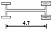 |
| B |  |  |
| C |  | 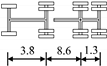 |
| D |  |  |
| E |  | 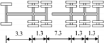 |
| F |  |  |
| G |  |  |
| Vehicle Type | Mean Value of Axle Weight Ratio | |||||
|---|---|---|---|---|---|---|
| Axle 1 | Axle 2 | Axle 3 | Axle 4 | Axle 5 | Axle 6 | |
| A | 0.392 | 0.608 | - | - | - | - |
| B | 0.264 | 0.266 | 0.470 | - | - | - |
| C | 0.185 | 0.207 | 0.291 | 0.317 | - | - |
| D | 0.154 | 0.274 | 0.199 | 0.184 | 0.190 | - |
| E | 0.109 | 0.138 | 0.204 | 0.193 | 0.178 | 0.177 |
| G | 0.392 | 0.608 | - | - | - | - |
| Variable | Description | Distribution Type | Mean Value | Standard Deviation |
|---|---|---|---|---|
| EICS | Lognormal | 0.15 | 0.1 | |
| Deterministic | 9.282 × 10⁸ | - | ||
| Material-related parameter | Normal | −27.76 | 0.23 | |
| Multiplier for crack geometric factor | Normal | 1 | 0.1 | |
| Hyperparameters of parent-nodes | Normal | 0 | 1 | |
| Standard deviation of observation error | Deterministic | 5 | - |
Publisher’s Note: MDPI stays neutral with regard to jurisdictional claims in published maps and institutional affiliations. |
© 2022 by the authors. Licensee MDPI, Basel, Switzerland. This article is an open access article distributed under the terms and conditions of the Creative Commons Attribution (CC BY) license (https://creativecommons.org/licenses/by/4.0/).
Share and Cite
Xu, Y.; Zhu, B.; Zhang, Z.; Chen, J. Hierarchical Dynamic Bayesian Network-Based Fatigue Crack Propagation Modeling Considering Initial Defects. Sensors 2022, 22, 6777. https://doi.org/10.3390/s22186777
Xu Y, Zhu B, Zhang Z, Chen J. Hierarchical Dynamic Bayesian Network-Based Fatigue Crack Propagation Modeling Considering Initial Defects. Sensors. 2022; 22(18):6777. https://doi.org/10.3390/s22186777
Chicago/Turabian StyleXu, Yang, Bin Zhu, Zheng Zhang, and Jiahui Chen. 2022. "Hierarchical Dynamic Bayesian Network-Based Fatigue Crack Propagation Modeling Considering Initial Defects" Sensors 22, no. 18: 6777. https://doi.org/10.3390/s22186777
APA StyleXu, Y., Zhu, B., Zhang, Z., & Chen, J. (2022). Hierarchical Dynamic Bayesian Network-Based Fatigue Crack Propagation Modeling Considering Initial Defects. Sensors, 22(18), 6777. https://doi.org/10.3390/s22186777