Author Contributions
Conceptualization, S.-C.Y.; data curation, C.-H.W.; formal analysis, C.-H.W. and C.-H.H.; funding acquisition, C.-H.W.; investigation, S.-C.Y. and Y.-S.C.; methodology, C.-H.H. and T.-P.C.; project administration, S.-C.Y.; resources, C.-H.W., C.-H.H. and Y.-S.C.; software, T.-P.C.; supervision, C.-H.W.; writing—original draft, S.-C.Y., C.-H.W. and T.-P.C.; writing—review & editing, C.-H.W. and Y.-S.C. All authors have read and agreed to the published version of the manuscript.
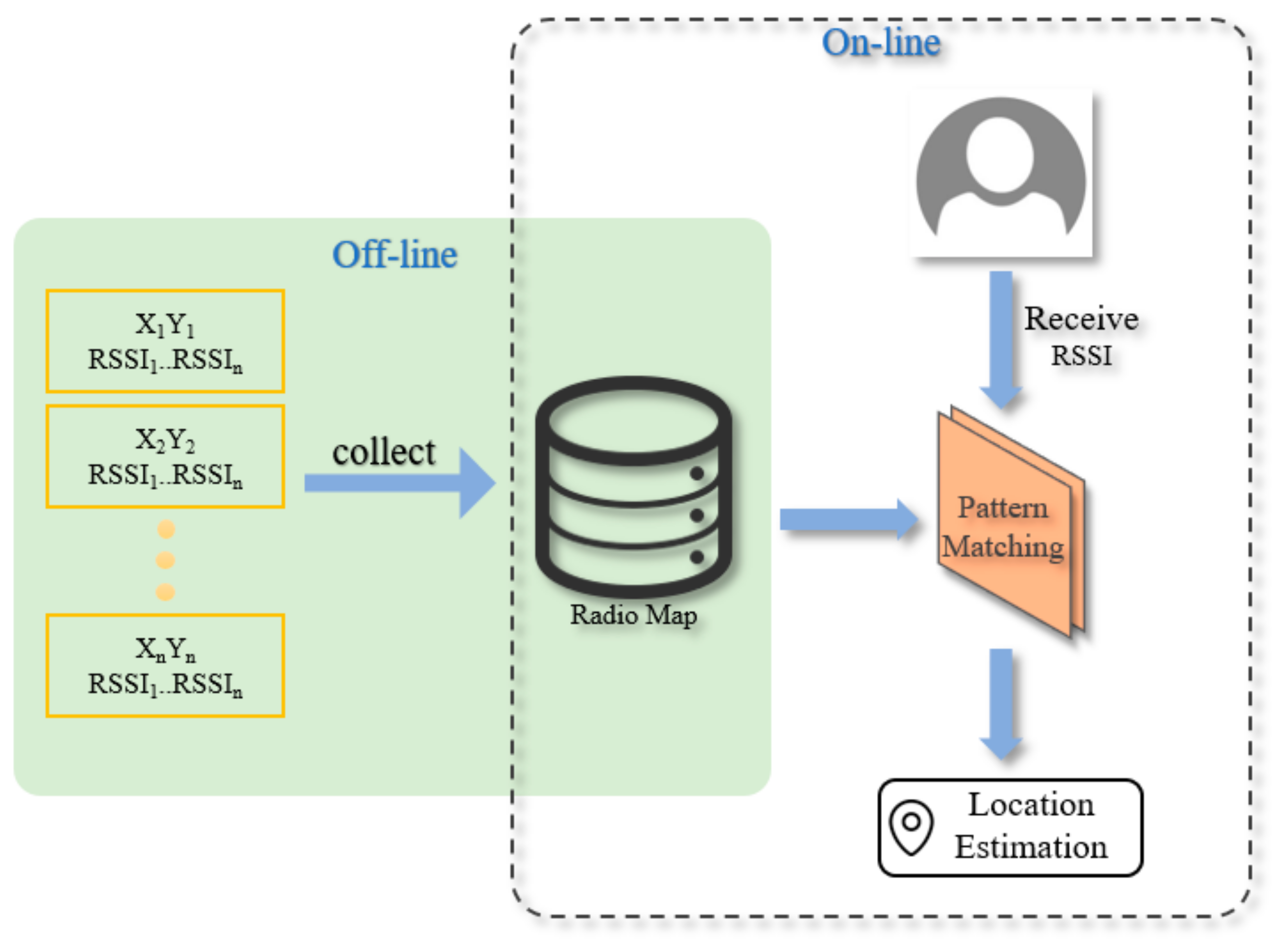
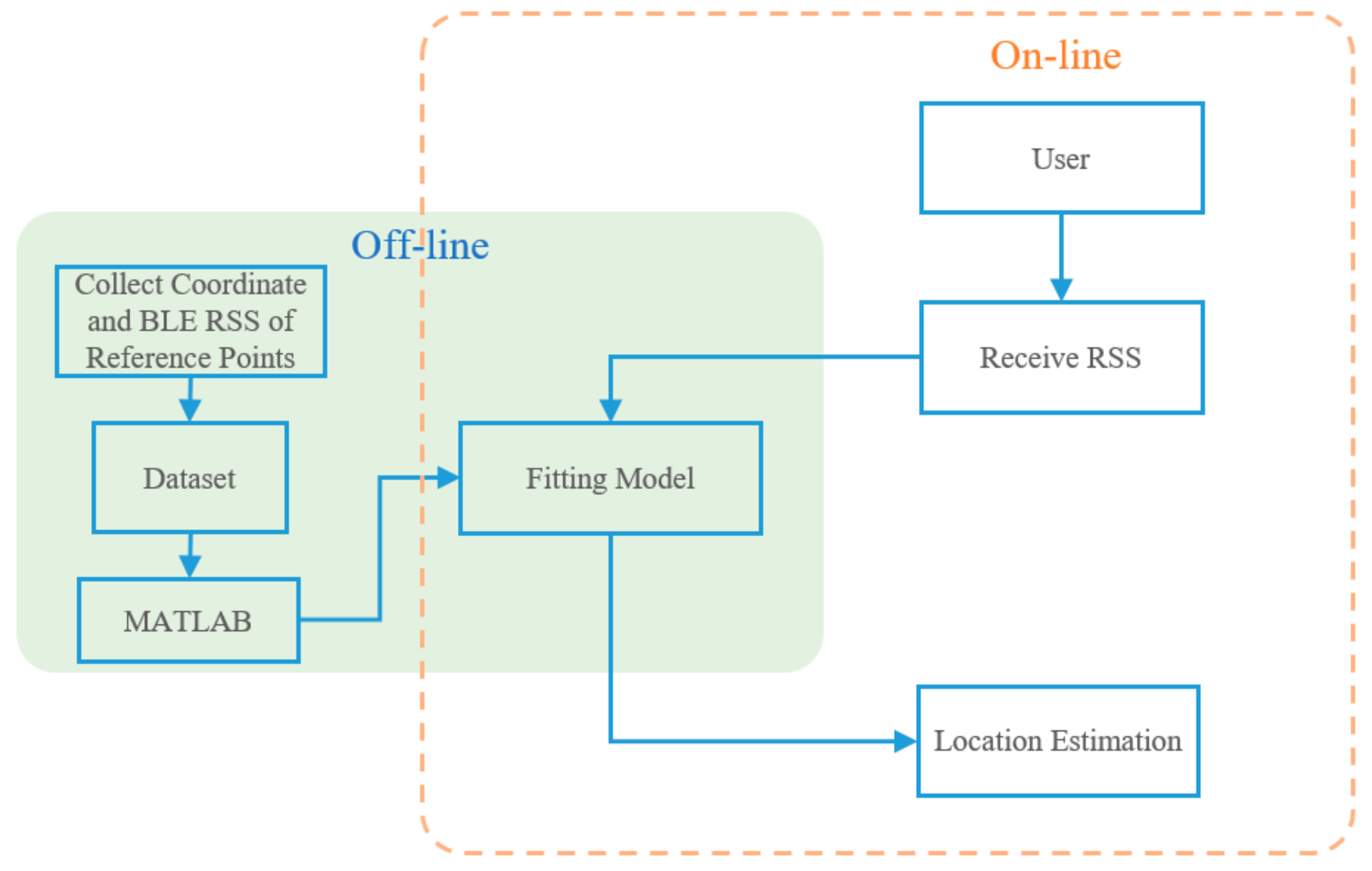
Figure 1.
RADAR Positioning Technology Flowchart [
2].
Figure 1.
RADAR Positioning Technology Flowchart [
2].
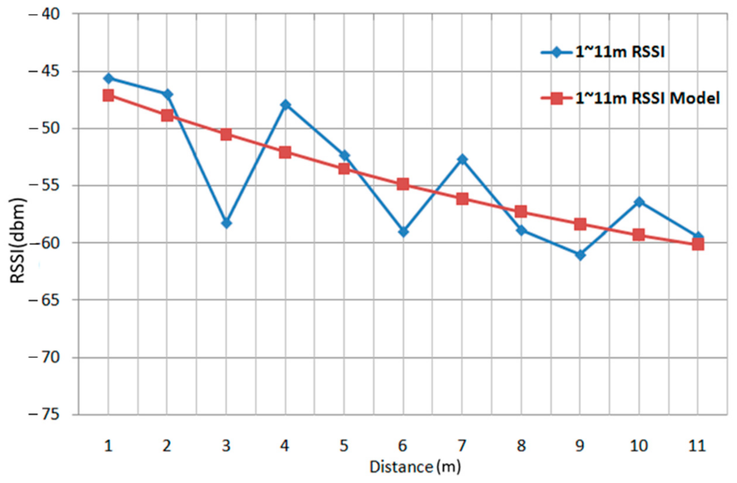
Figure 2.
Graph of Relationship between Signal Intensity and Distance [
6].
Figure 2.
Graph of Relationship between Signal Intensity and Distance [
6].
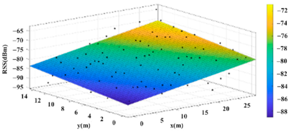
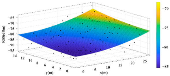
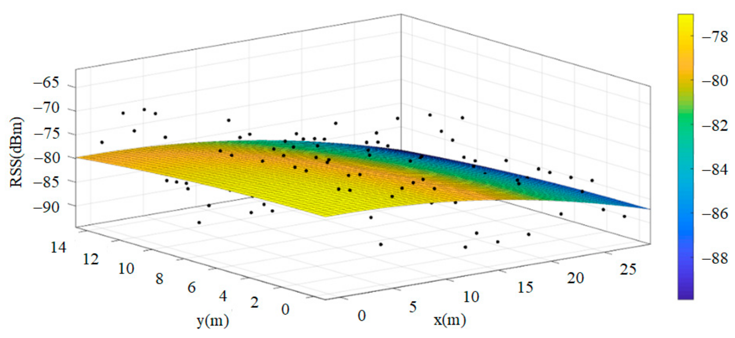
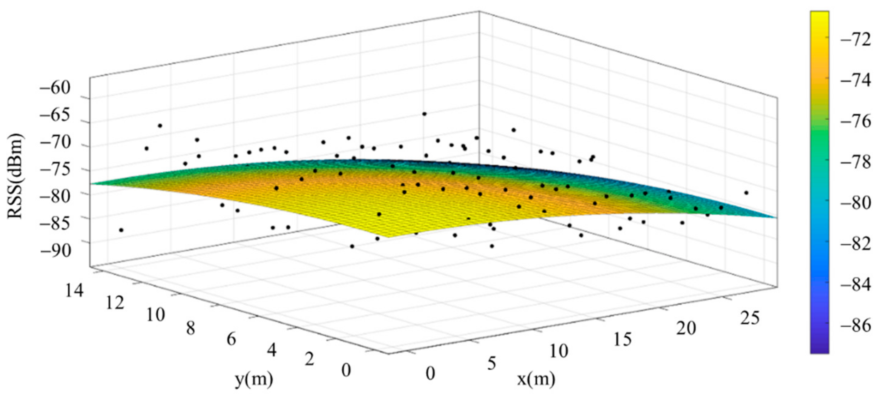
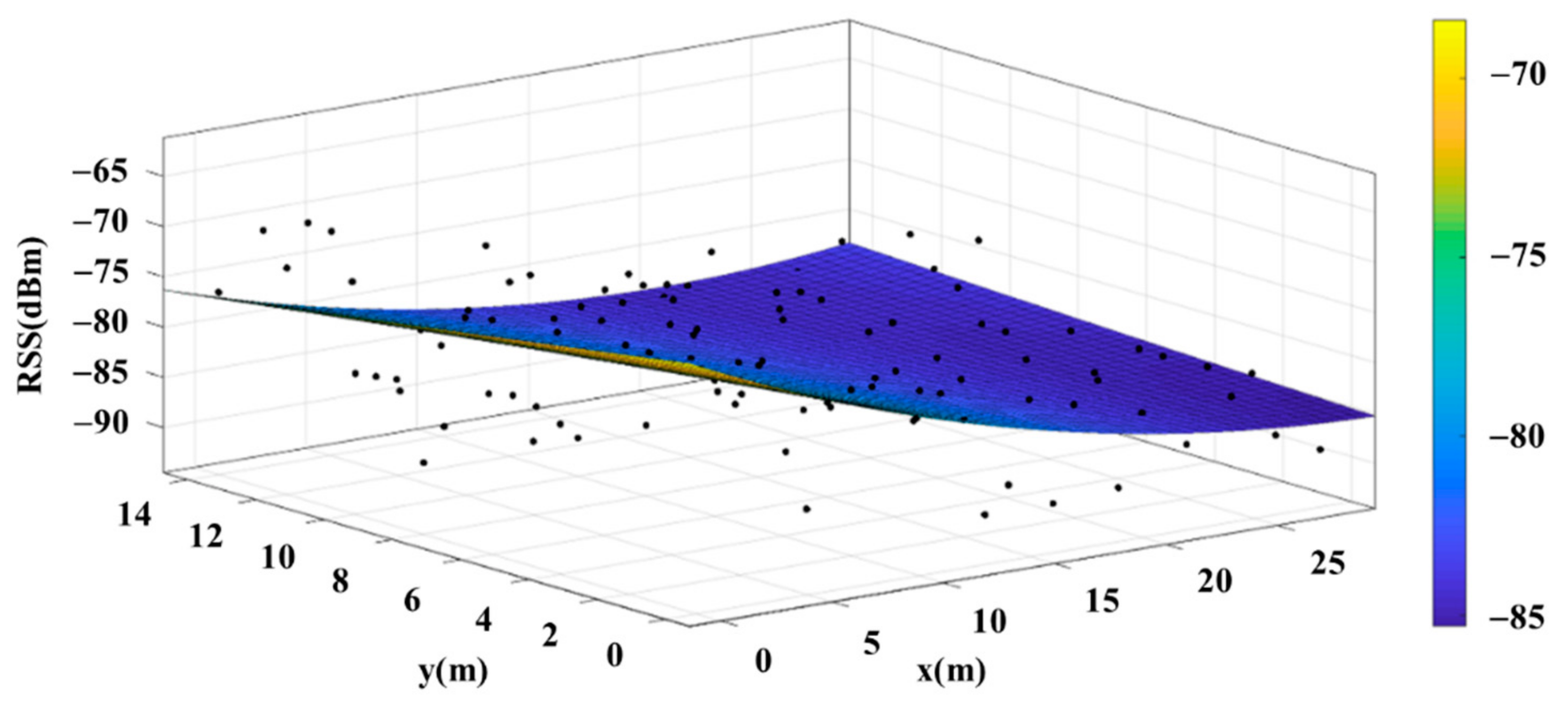
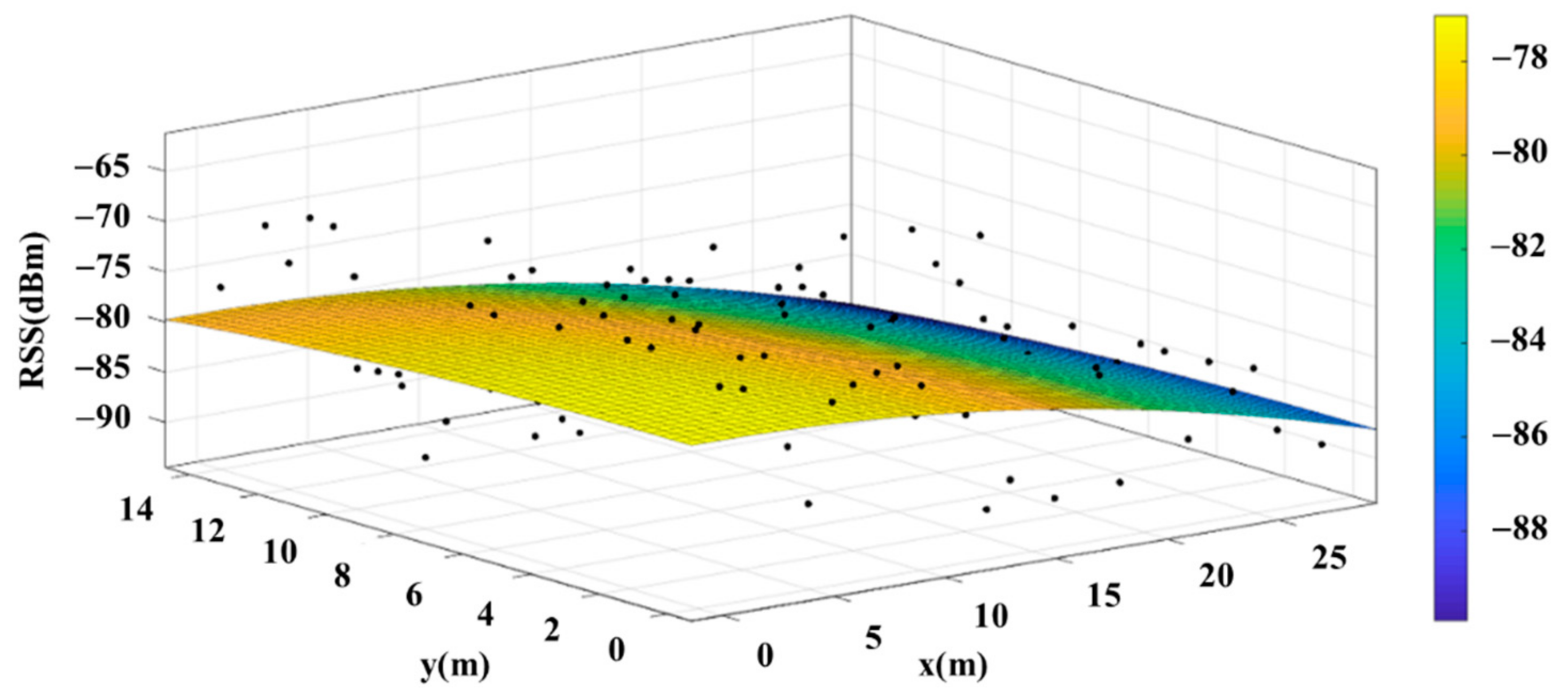
Figure 3.
Actual Signal Intensity Distribution and the Planar Model.
Figure 3.
Actual Signal Intensity Distribution and the Planar Model.
Figure 4.
Schematic Diagram of System Architecture.
Figure 4.
Schematic Diagram of System Architecture.
Figure 5.
System Flowchart for This Study.
Figure 5.
System Flowchart for This Study.
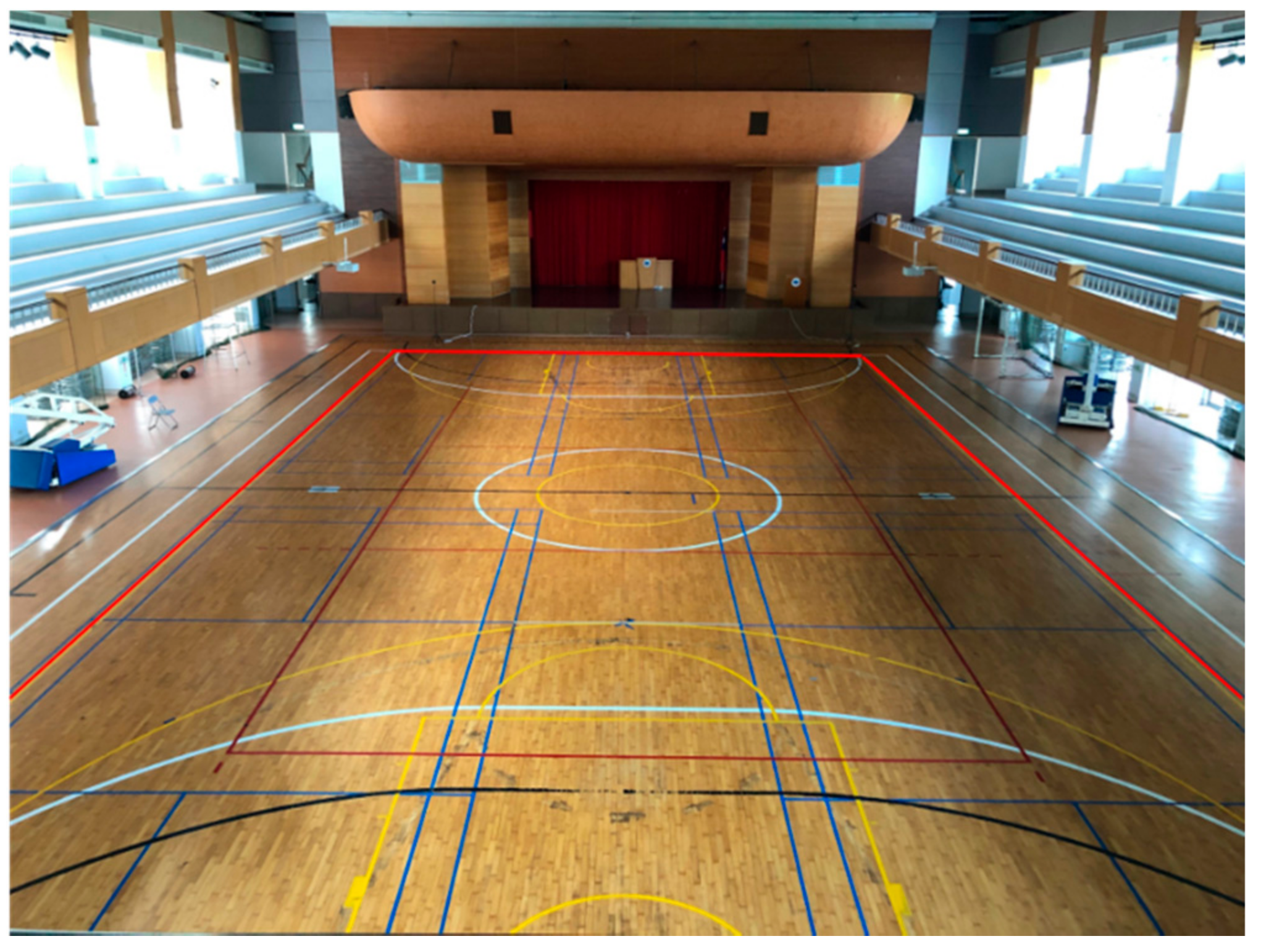
Figure 6.
Experimental Environment–Basketball Court.
Figure 6.
Experimental Environment–Basketball Court.
Figure 7.
Schematic Diagram of Planned Reference Points in the Environment.
Figure 7.
Schematic Diagram of Planned Reference Points in the Environment.
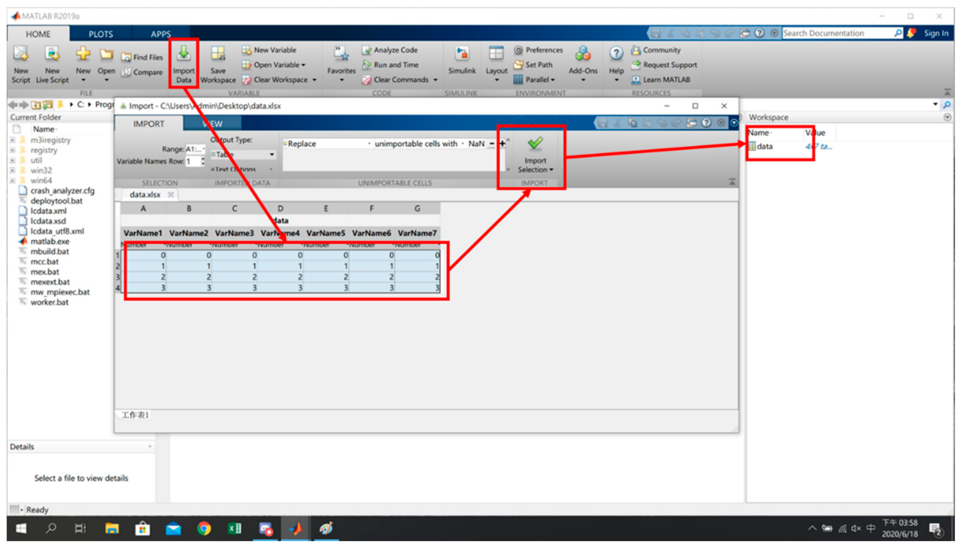
Figure 8.
Input of Reference Point Data into MATLAB [
17].
Figure 8.
Input of Reference Point Data into MATLAB [
17].
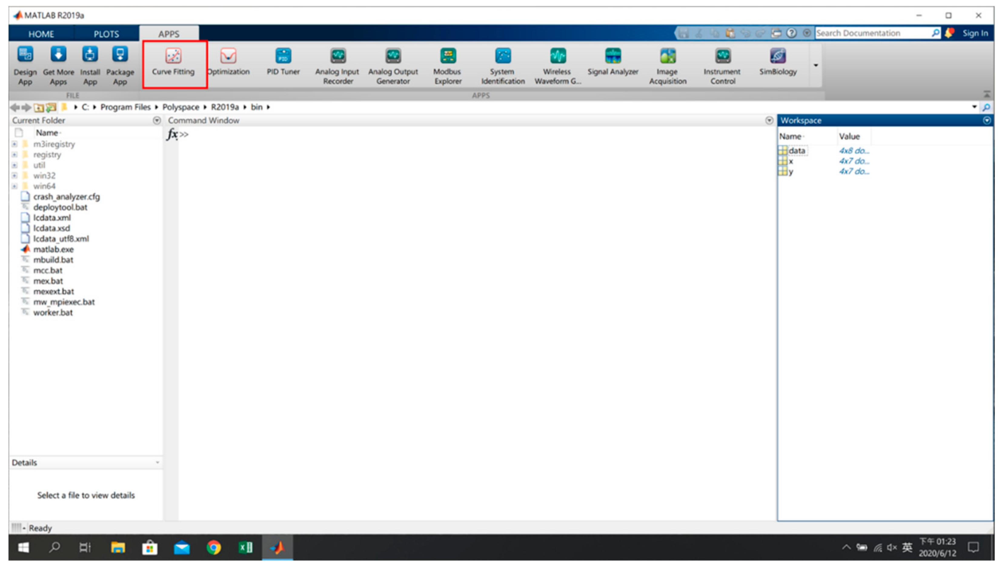
Figure 9.
Curve Fitting Tool.
Figure 9.
Curve Fitting Tool.
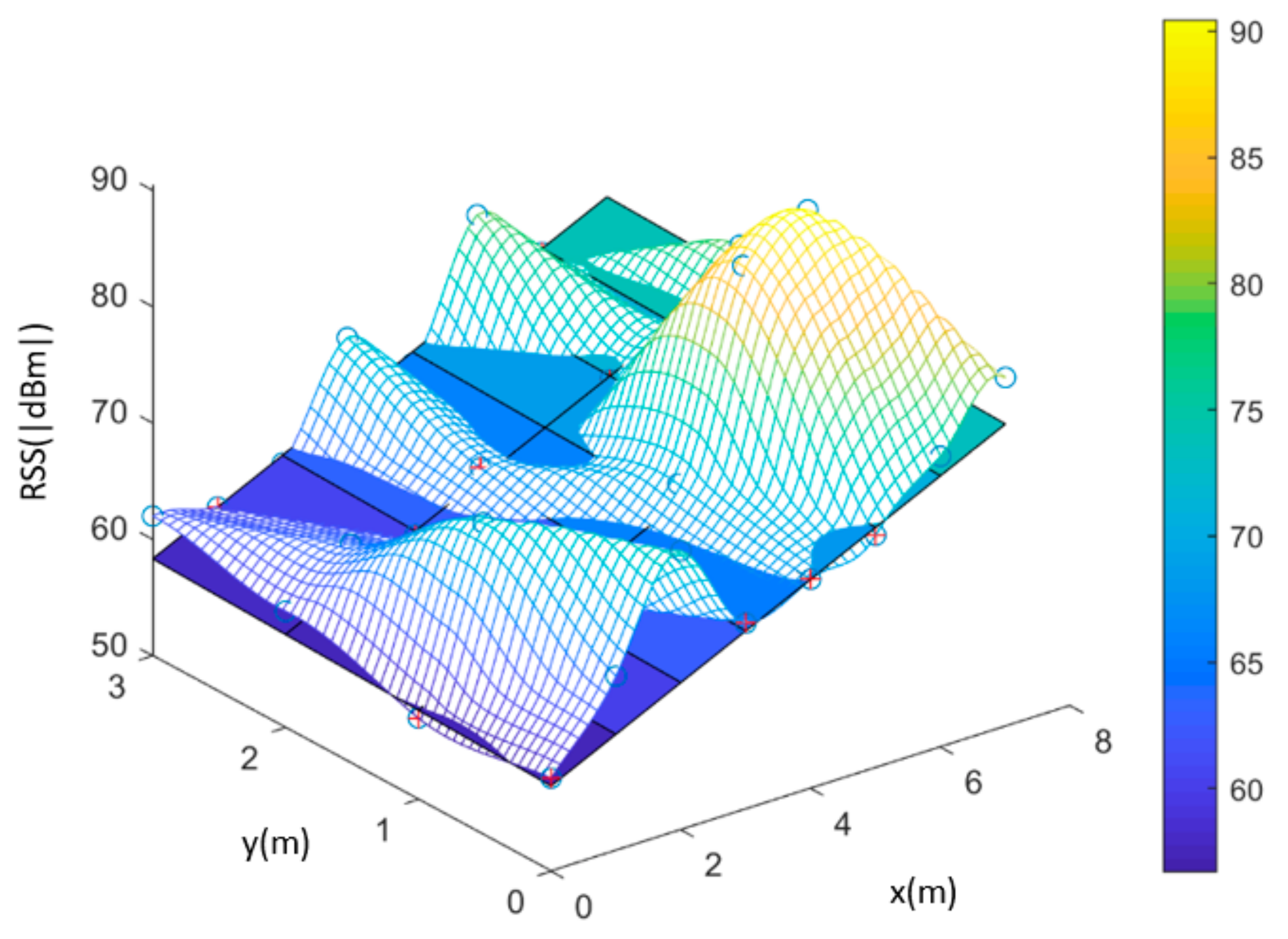
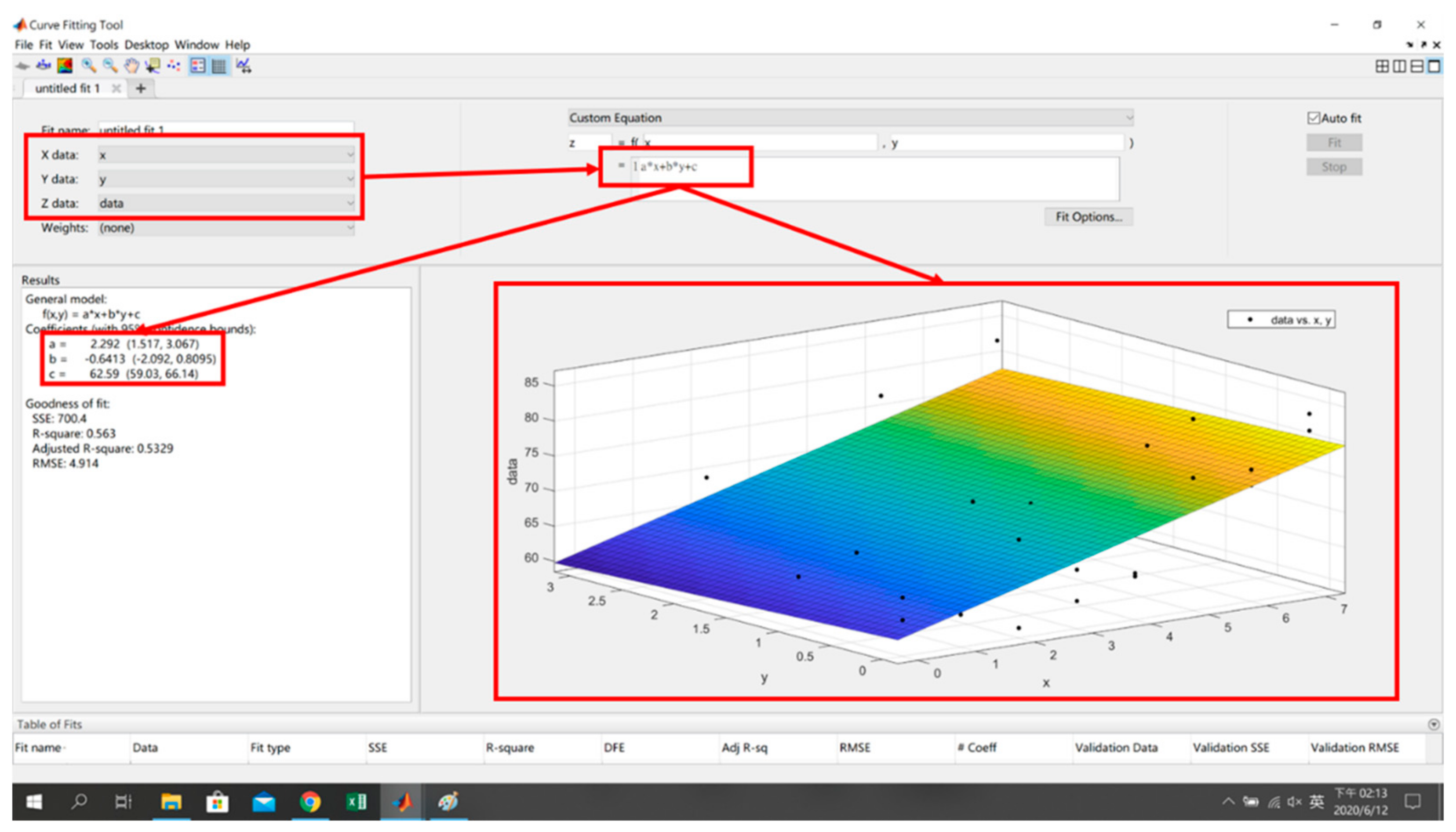
Figure 10.
Planar Model and Equation Generation.
Figure 10.
Planar Model and Equation Generation.
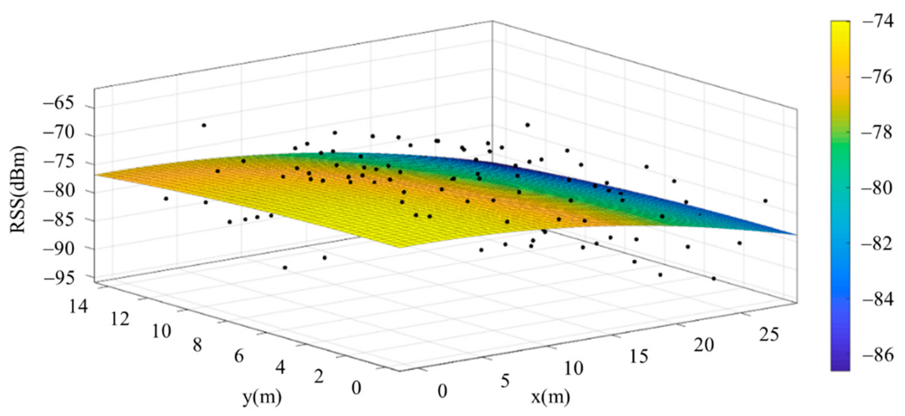
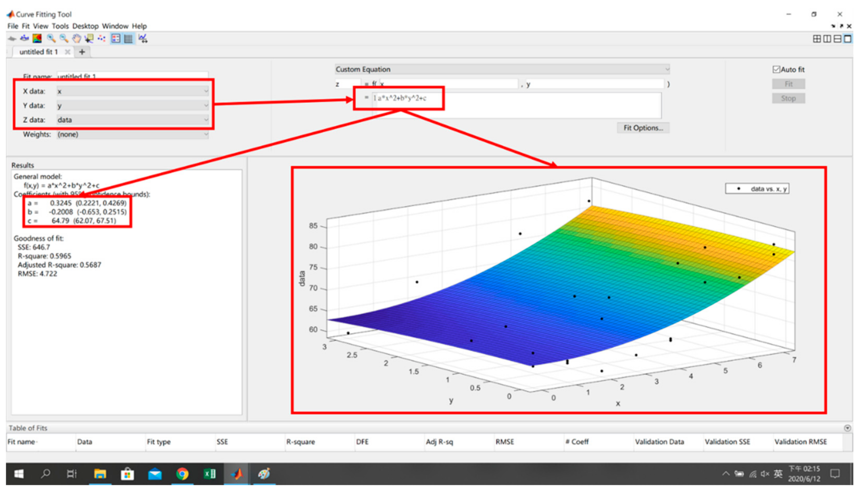
Figure 11.
Fitting Model and Equation Generation.
Figure 11.
Fitting Model and Equation Generation.
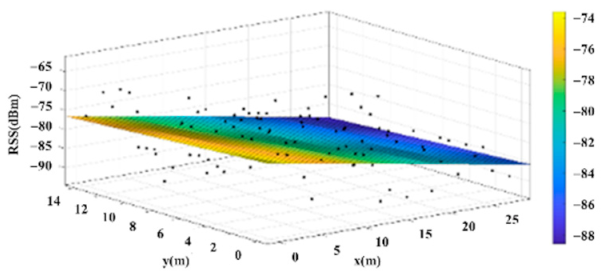
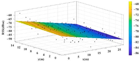
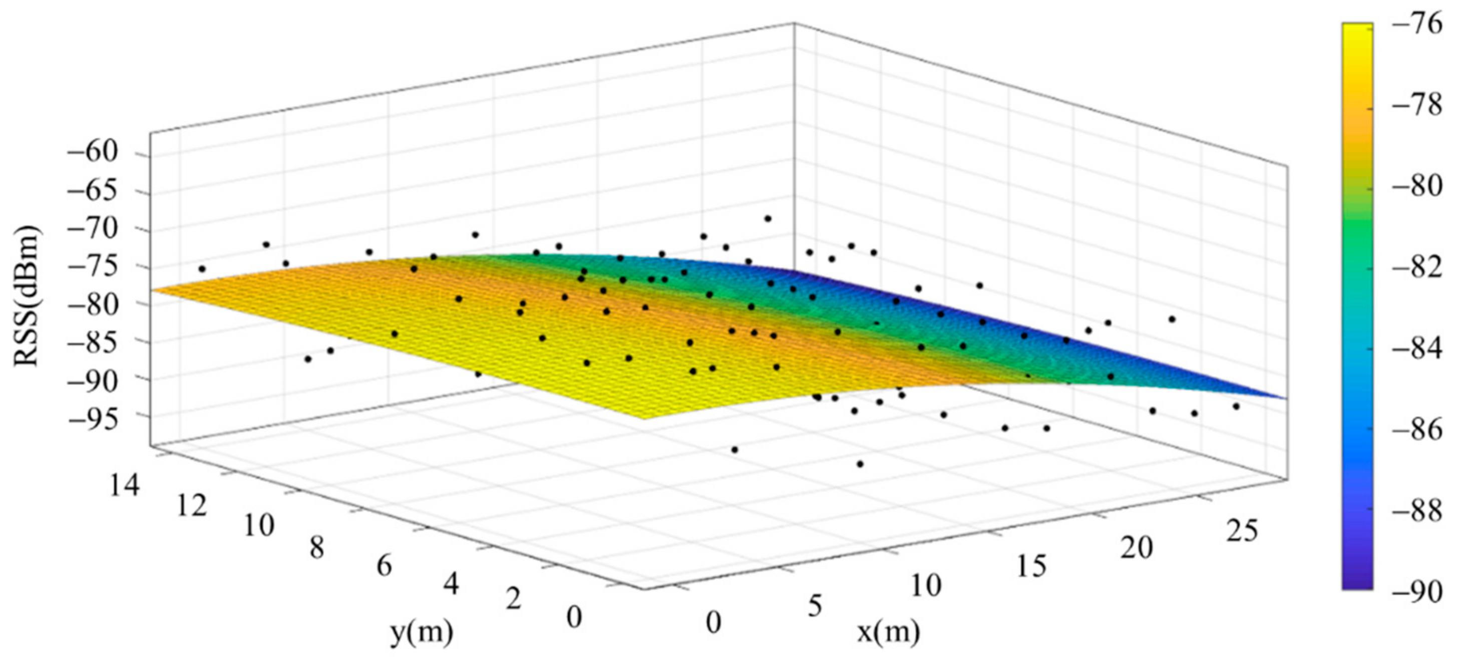
Figure 12.
Fitting Model Generated for Base Station A.
Figure 12.
Fitting Model Generated for Base Station A.
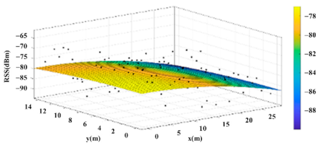
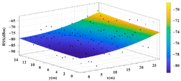
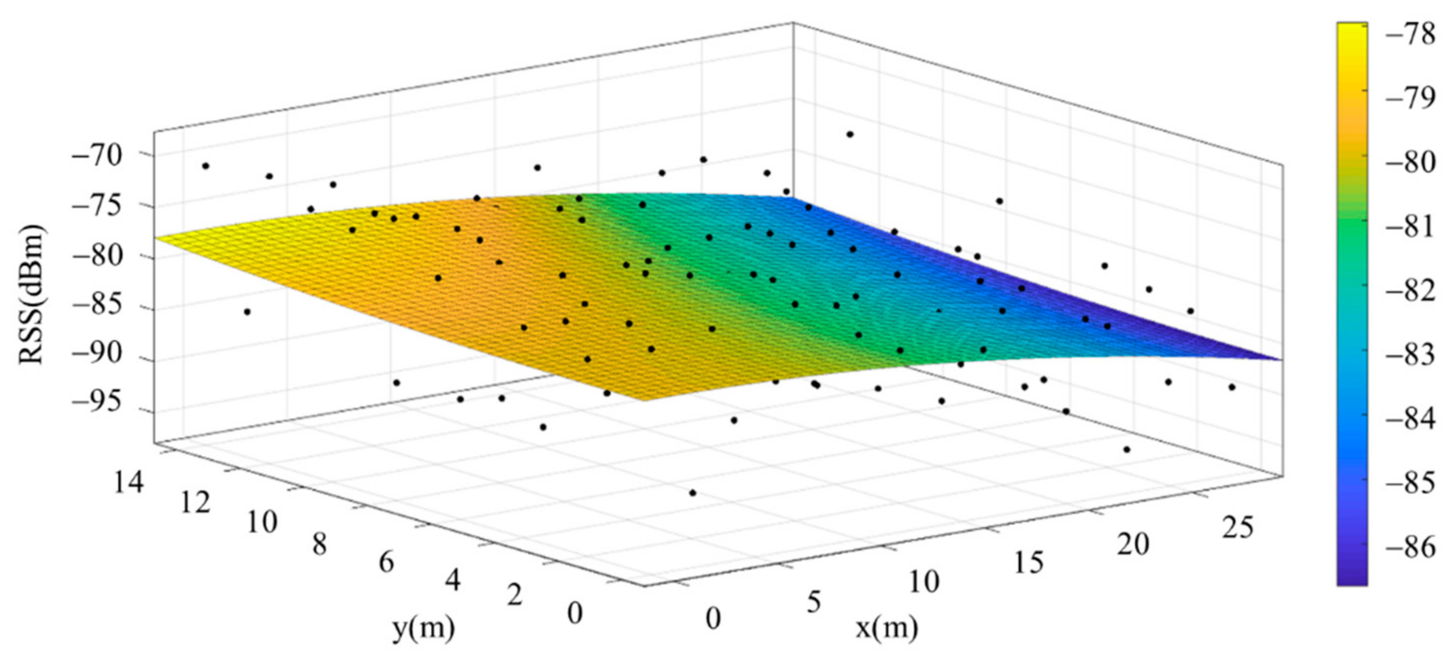
Figure 13.
Fitting Model Generated for Base Station B.
Figure 13.
Fitting Model Generated for Base Station B.
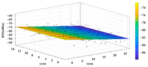
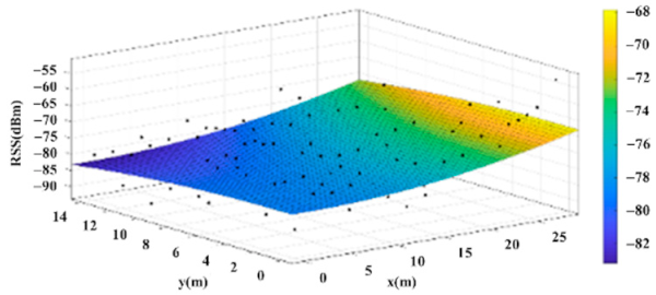
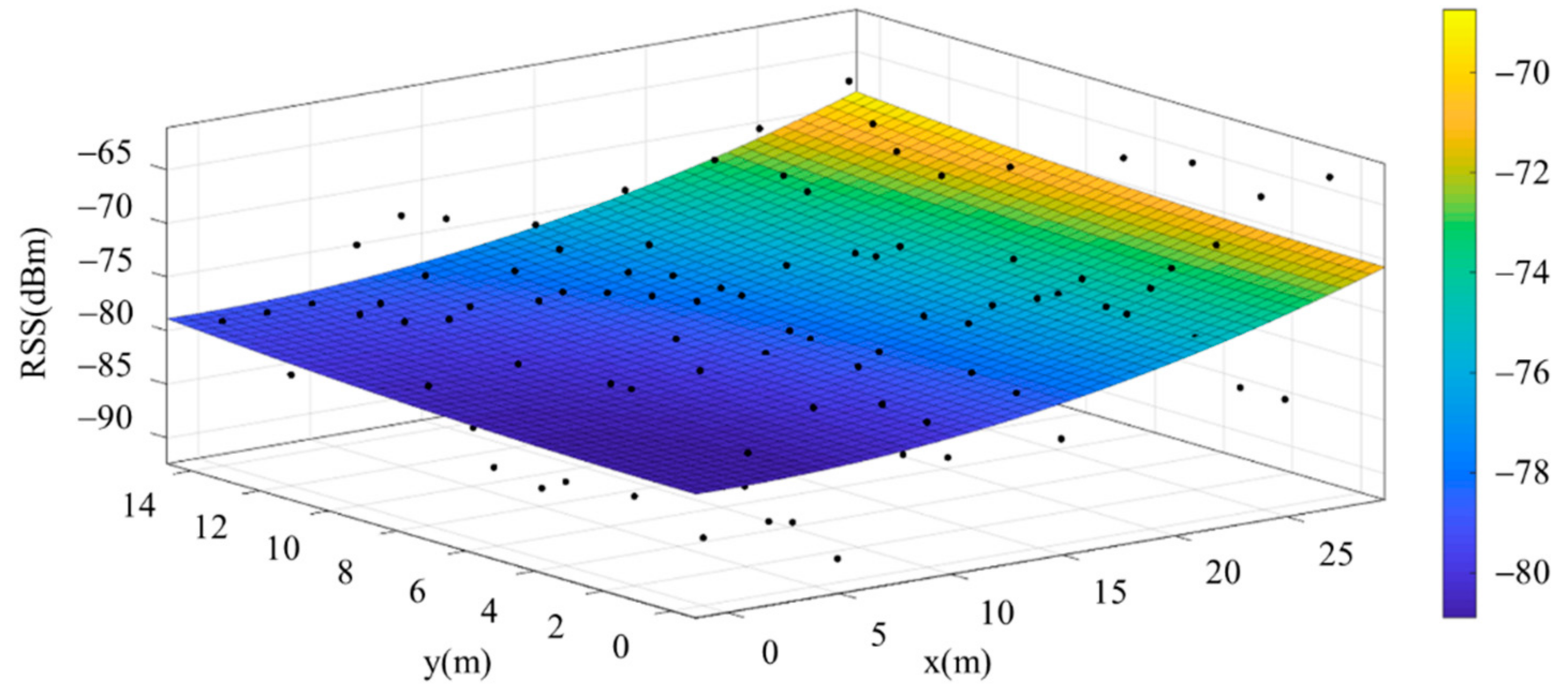
Figure 14.
Fitting Model Generated for Base Station C.
Figure 14.
Fitting Model Generated for Base Station C.
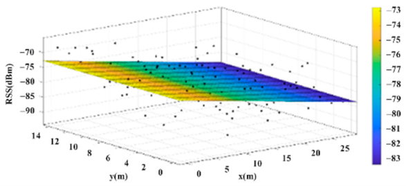
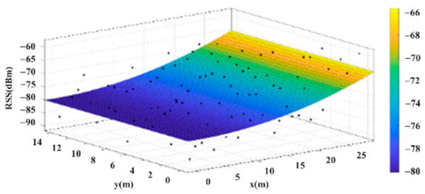
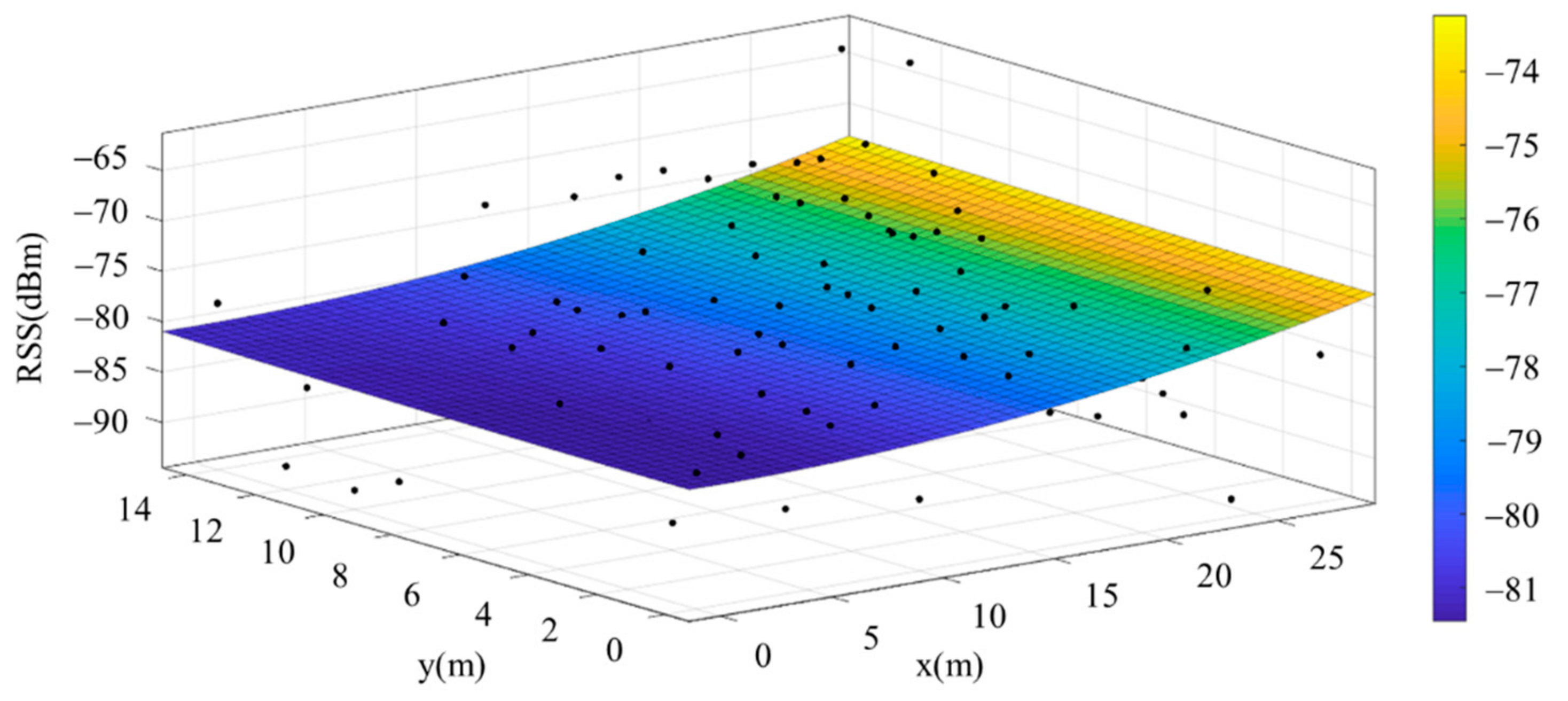
Figure 15.
Fitting Model Generated for Base Station D.
Figure 15.
Fitting Model Generated for Base Station D.
Figure 16.
Fitting Model for Same Base Station Using Data Collected Facing East.
Figure 16.
Fitting Model for Same Base Station Using Data Collected Facing East.
Figure 17.
Fitting Model for Same Base Station Using Data Collected Facing West.
Figure 17.
Fitting Model for Same Base Station Using Data Collected Facing West.
Figure 18.
Fitting Model for Same Base Station Using Data Collected Facing South.
Figure 18.
Fitting Model for Same Base Station Using Data Collected Facing South.
Figure 19.
Fitting Model for Same Base Station Using Data Collected Facing North.
Figure 19.
Fitting Model for Same Base Station Using Data Collected Facing North.
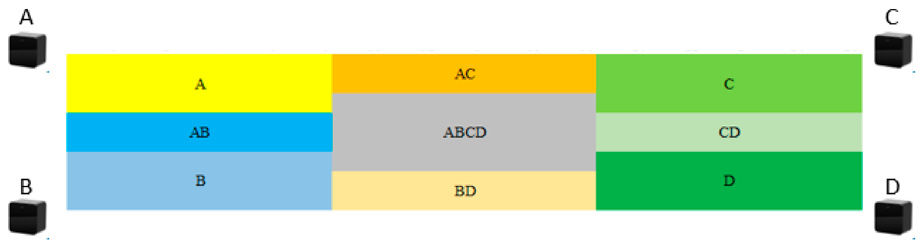
Figure 20.
Distribution of Determination Blocks According to the Closest Base Station.
Figure 20.
Distribution of Determination Blocks According to the Closest Base Station.
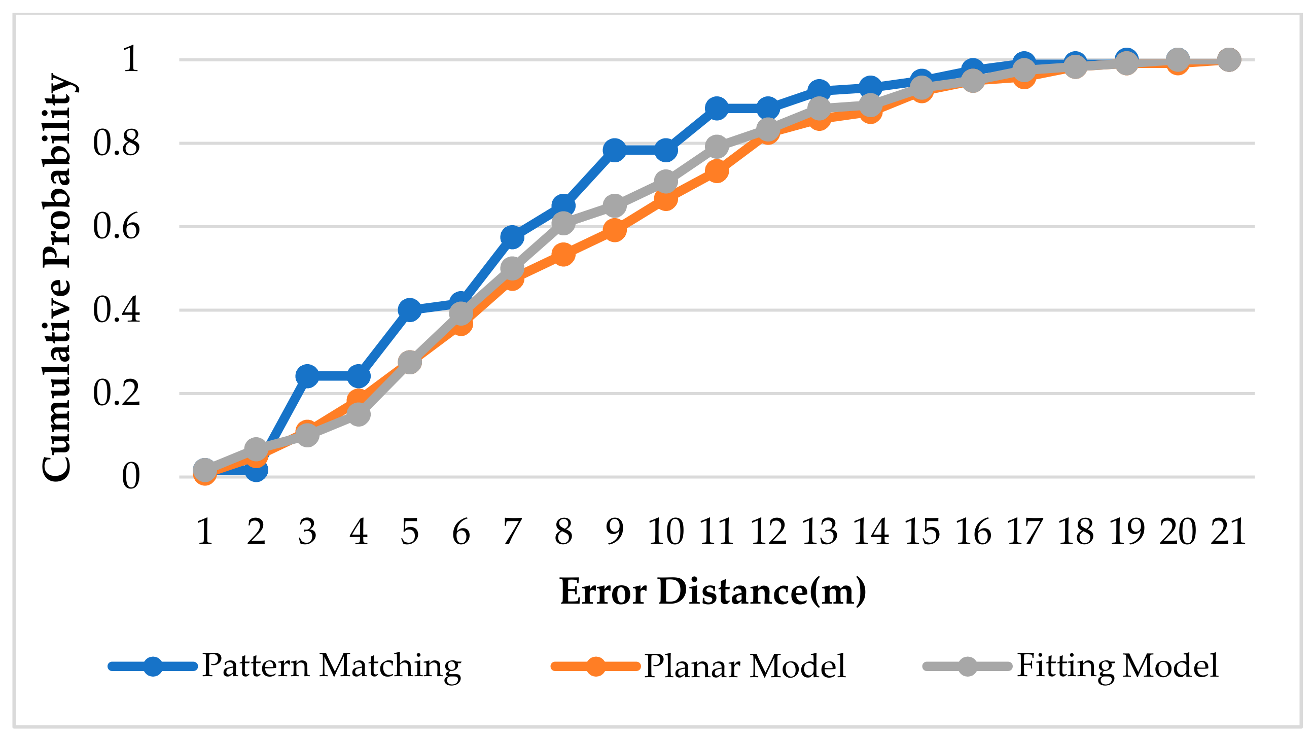
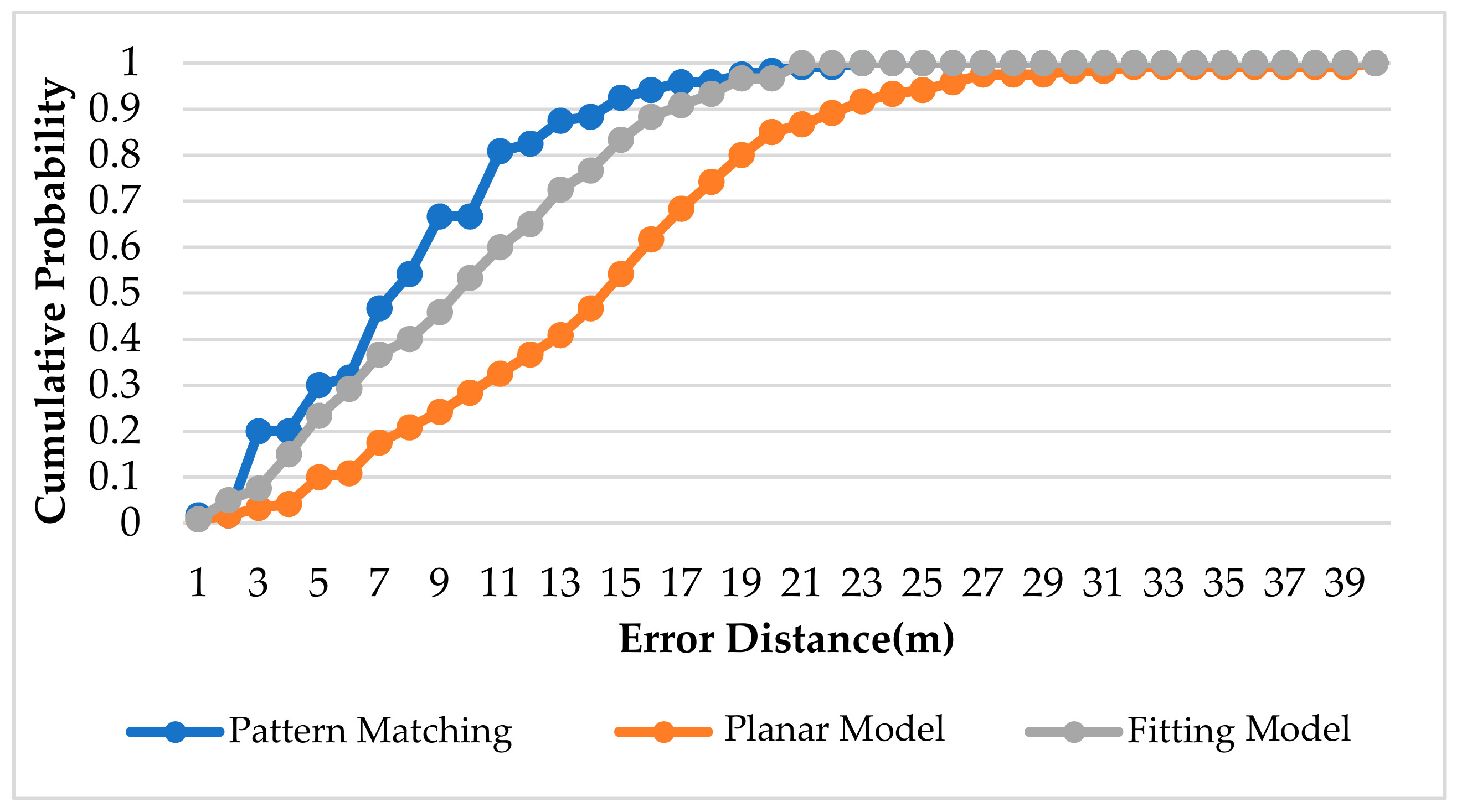
Figure 21.
CDF for Original Data in Basketball Court.
Figure 21.
CDF for Original Data in Basketball Court.
Figure 22.
CDF for Area Determination in Basketball Court.
Figure 22.
CDF for Area Determination in Basketball Court.
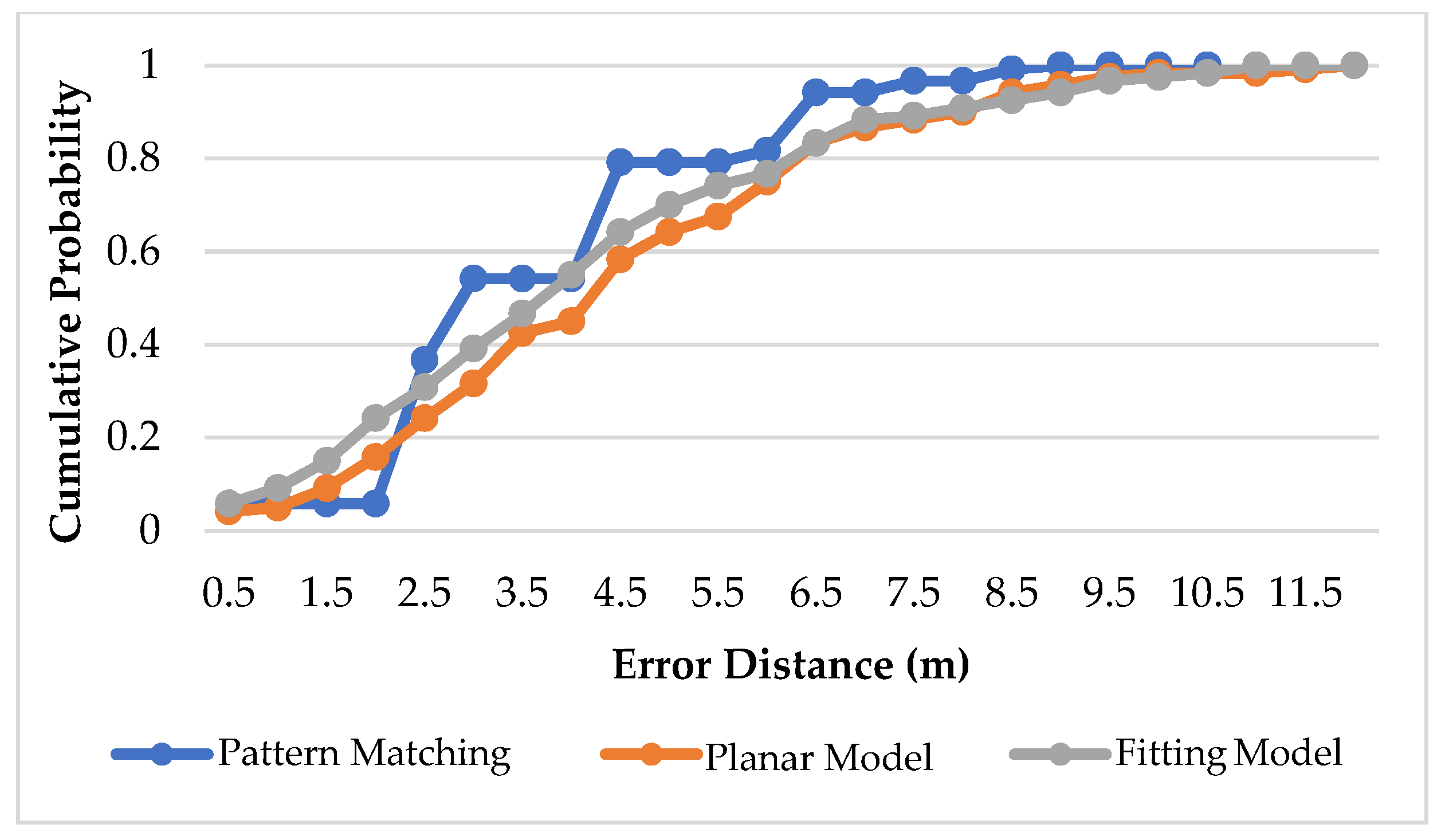
Figure 23.
CDF for Optimal Area in Basketball Court.
Figure 23.
CDF for Optimal Area in Basketball Court.
Figure 24.
Model Generated Using Simplified Surface Equations.
Figure 24.
Model Generated Using Simplified Surface Equations.
Figure 25.
Model Generated Using Surface Normalizing Equations.
Figure 25.
Model Generated Using Surface Normalizing Equations.
Table 1.
Comparisons of characteristics in various positioning technologies [
16].
Table 1.
Comparisons of characteristics in various positioning technologies [
16].
| Wireless Position System | Localization Technique | Range | Accuracy |
|---|
| DOLPHIN (RF with Ultrasonic) | ToA, trilateration | Indoor | 2 cm |
| RFID/INS | RSS/INS | Indoor | 2 m |
| UWB | TDoA/ToA, trilateration | 15 m | 10 cm |
| RFID/FPM | RSS/INS | Indoor | 1.7 m |
| Land Marc | RSS, triangulation | 50 m | 1~2 m |
| GPS | ToA, trilateration | Global | 1~5 m |
| Radar | RSS, triangulation | Indoor | Indoor |
| Cricket | ToA, trilateration | 10 m | 2 cm |
| Active Bats | ToA, trilateration | 50 m | 9 cm |
| Active Badge | ToA, trilateration | 5 m | 7 cm |
| COMPASS | RSS, triangulation | 15 m | 1.65 m |
| WhereNet (RF) | RSS, triangulation | 20 m | 2~3 m |
| LiFS | Fingerprinting database | Indoor | 9 m |
| Bluetooth | RSSI fingerprinting/RSSI theoretical propagation model | Indoor | 2~5 m |
Table 2.
Individual Fitting Model Equations for the Different Base Stations.
Table 2.
Individual Fitting Model Equations for the Different Base Stations.
| Base Station | Fitting Model Equation |
|---|
| A | |
| B | |
| C | |
| D | |
Table 3.
Individual Fitting Model Equations for the Same Base Station Using Data Collected from Different Directions.
Table 3.
Individual Fitting Model Equations for the Same Base Station Using Data Collected from Different Directions.
| Direction Faced | Fitting Model Equation |
|---|
| East | |
| West | |
| South | |
| North | |
Table 4.
Models and Equations Generated from the Four Directions in the Experimental Environment for Base Station A.
Table 5.
Models and Equations Generated from the Four Directions in the Experimental Environment for Base Station B.
Table 6.
Models and Equations Generated from the Four Directions in the Experimental Environment for Base Station C.
Table 7.
Models and Equations Generated from the Four Directions in the Experimental Environment for Base Station D.
Table 8.
Comparison of Average Positioning Error on the Basketball Court.
Table 8.
Comparison of Average Positioning Error on the Basketball Court.
| Method | Original | Area | Optimal |
|---|
| Signal Pattern Matching | 7.77 | 6.63 | 3.56 |
| Planar Model | 14.15 | 8.15 | 4.34 |
| Fitting Model | 9.7 | 7.82 | 4.02 |
Table 9.
Improvement by Fitting Model Compared to Planar Model Ratios.
Table 9.
Improvement by Fitting Model Compared to Planar Model Ratios.
| Environment | Original | Area | Optimal |
|---|
| Basketball Court (large environment) | 31% | 4% | 7% |
Table 10.
Average Positioning Error Distance for Different Number of Reference Points.
Table 10.
Average Positioning Error Distance for Different Number of Reference Points.
| Method (No. Reference Points, Spacing) | Original | Area |
|---|
| Planar Model (120, 2 m) | 14.15 | 8.15 |
| Planar Model (32, 4 m) | 13.15 | 7.88 |
| Planar Model (8, 8 m) | 13.12 | 7.11 |
| Fitting Model (120, 2 m) | 9.7 | 7.82 |
| Fitting Model (32, 4 m) | 9.5 | 7.4 |
| Fitting Model (8, 8 m) | 11.15 | 6.66 |


