
Monitoring Fish Freshness in Real Time under Realistic Conditions through a Single Metal Oxide Gas Sensor

 , , ,
, , ,  and
and 
Abstract
:1. Introduction
2. Materials and Methods
2.1. Tested Samples
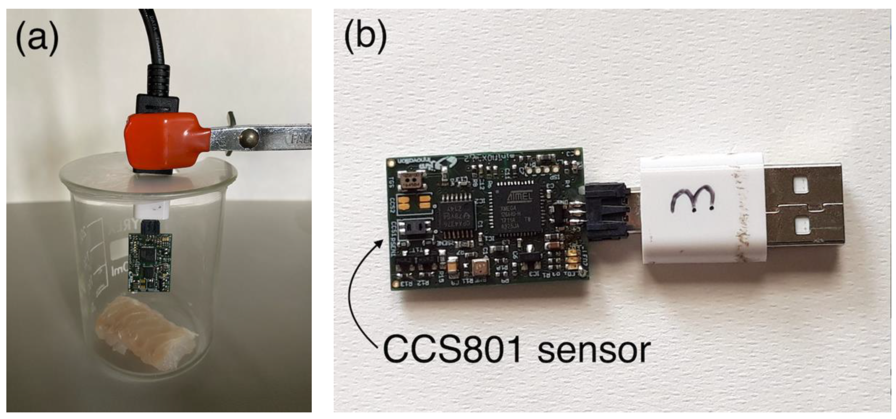
2.2. Sensing System
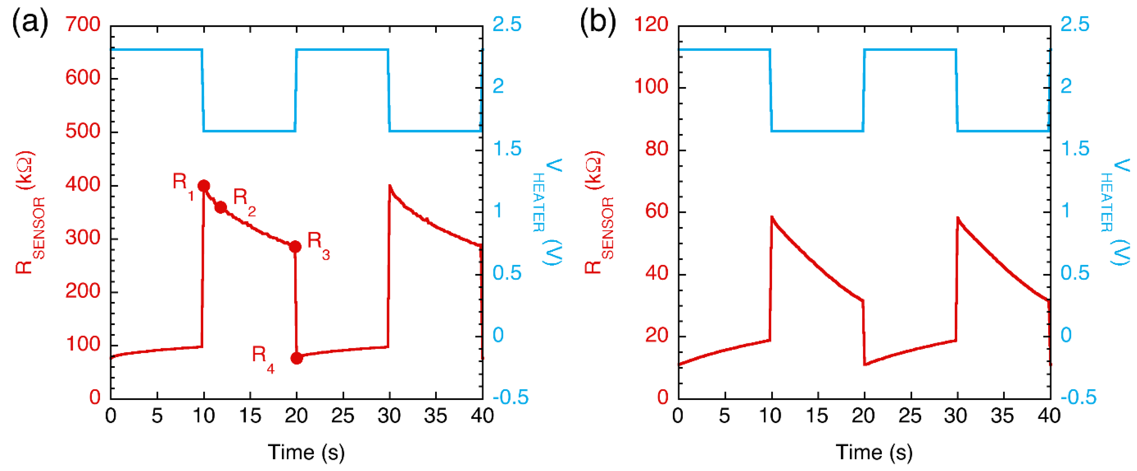
- R1: the sensor resistance measured during the second sampling time in which VHEATER is in the low state. Considering that the thermal time constants of microhotplate-based sensors are of the order of a few milliseconds [38], a single sampling time (0.2 s) allowed for reaching a steady-state temperature.
- R2: the sensor resistance measured 2 s after the VHEATER was switched from the high to the low state.
- R3: the sensor resistance measured during the last sampling time in which VHEATER was kept in the low state.
- R4: the sensor resistance during the second sampling time in which the VHEATER was in the high state.
- Delta-C = variation in RSENSOR measurements during the cold half-period, i.e., Delta-C = R1 − R3;
- Delta-CH = variation in RSENSOR measurements between the end of the cold half-period and the beginning of the next hot half-period, i.e., Delta-CH = R3 − R4;
- Ratio-CH = ratio between the RSENSOR measurements at the end of the cold half-period and at the beginning of the next hot half-period, i.e., Delta-CH = R3/R4;
- Slope-C = slope of the RSENSOR vs. time curve extrapolated during the initial stage of the cold half-period, i.e., Slope-C = (R1 − R2)/(t2 − t1), where the time interval is t2 − t1 = 2 s.
- Sample, as described in Table 1.
- Temperature kept during sensing test, as listed in Table 1.
- Time, which refers to the testing time, starting from T0 as described in Section 2.1.
- Total viable count (TVC), which was carried out at discrete times according to the procedure described in Section 2.3. As better detailed in Section 2.3 and further discussed in Section 3, it is not possible to have a continuous TVC. This characterization should be done at discrete times, and so far only a few measurements have the corresponding TVC label.
2.3. Microbiological Characterization
2.4. Chemical Characterization
3. Results and Discussion
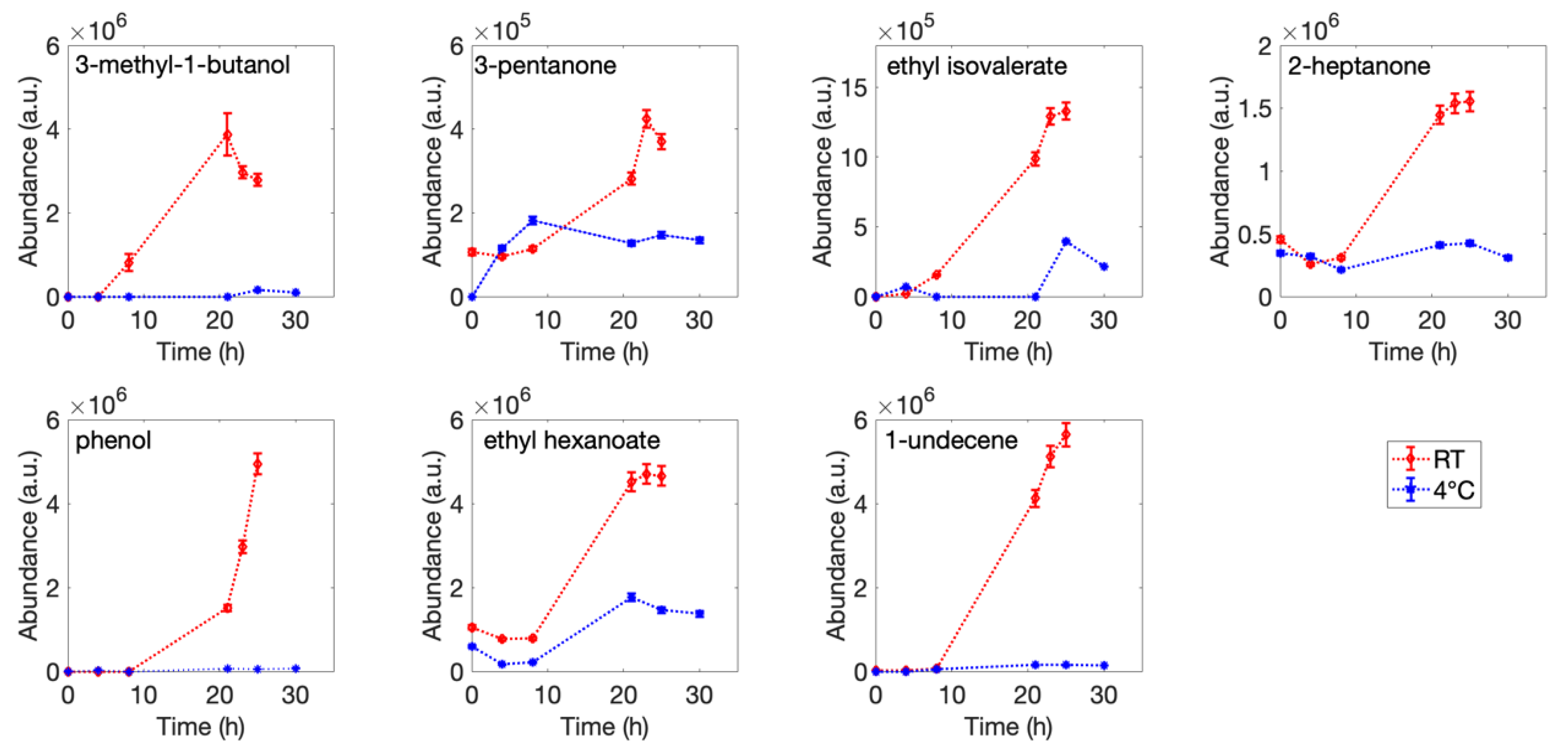
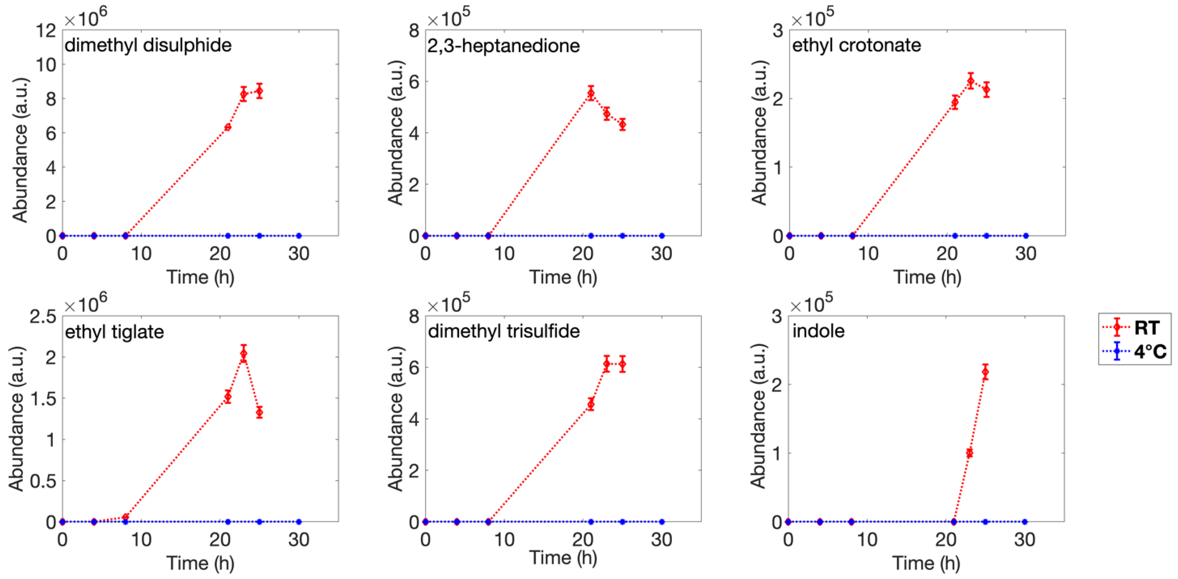
3.1. Headspace Analysis
3.2. Microbiological Analysis
3.3. Sensing System Characterization
4. Conclusions
Author Contributions
Funding
Institutional Review Board Statement
Informed Consent Statement
Data Availability Statement
Conflicts of Interest
References
- Health Protection Agency. Guidelines for Assessing the Microbiological Safety of Ready-to-Eat Foods Placed on the Market; Health Protection Agency: London, UK, 2009; p. 34.
- European Food Safety Authority and European Centre for Disease Prevention and Control (EFSA and ECDC). The European Union Summary Report on Trends and Sources of Zoonoses, Zoonotic Agents and Food-Borne Outbreaks in 2017. EFSA J. 2018, 16, e05500. [Google Scholar] [CrossRef]
- Potyrailo, R.A. Multivariable Sensors for Ubiquitous Monitoring of Gases in the Era of Internet of Things and Industrial Internet. Chem. Rev. 2016, 116, 11877–11923. [Google Scholar] [CrossRef]
- Morone, M.I.F. The Time Is Ripe for Food Spoilage Sensors. CEN Glob. Enterp. 2020, 98, 16–19. [Google Scholar] [CrossRef]
- Gram, L.; Dalgaard, P. Fish Spoilage Bacteria—Problems and Solutions. Curr. Opin. Biotechnol. 2002, 13, 262–266. [Google Scholar] [CrossRef]
- Chang, L.-Y.; Chuang, M.-Y.; Zan, H.-W.; Meng, H.-F.; Lu, C.-J.; Yeh, P.-H.; Chen, J.-N. One-Minute Fish Freshness Evaluation by Testing the Volatile Amine Gas with an Ultrasensitive Porous-Electrode-Capped Organic Gas Sensor System. ACS Sens. 2017, 2, 531–539. [Google Scholar] [CrossRef]
- Ma, Z.; Chen, P.; Cheng, W.; Yan, K.; Pan, L.; Shi, Y.; Yu, G. Highly Sensitive, Printable Nanostructured Conductive Polymer Wireless Sensor for Food Spoilage Detection. Nano Lett. 2018, 18, 4570–4575. [Google Scholar] [CrossRef]
- Cho, Y.H.; Kang, Y.C.; Lee, J.-H. Highly Selective and Sensitive Detection of Trimethylamine Using WO3 Hollow Spheres Prepared by Ultrasonic Spray Pyrolysis. Sens. Actuators B Chem. 2013, 176, 971–977. [Google Scholar] [CrossRef]
- Galstyan, V.; Ponzoni, A.; Kholmanov, I.; Natile, M.M.; Comini, E.; Sberveglieri, G. Highly Sensitive and Selective Detection of Dimethylamine through Nb-Doping of TiO2 Nanotubes for Potential Use in Seafood Quality Control. Sens. Actuators B Chem. 2020, 303, 127217. [Google Scholar] [CrossRef]
- Bhadra, S.; Narvaez, C.; Thomson, D.J.; Bridges, G.E. Non-Destructive Detection of Fish Spoilage Using a Wireless Basic Volatile Sensor. Talanta 2015, 134, 718–723. [Google Scholar] [CrossRef]
- Liu, B.; Gurr, P.A.; Qiao, G.G. Irreversible Spoilage Sensors for Protein-Based Food. ACS Sens. 2020, 5, 2903–2908. [Google Scholar] [CrossRef]
- Barandun, G.; Soprani, M.; Naficy, S.; Grell, M.; Kasimatis, M.; Chiu, K.L.; Ponzoni, A.; Güder, F. Cellulose Fibers Enable Near-Zero-Cost Electrical Sensing of Water-Soluble Gases. ACS Sens. 2019, 4, 1662–1669. [Google Scholar] [CrossRef]
- Xiang, J.; Su, Y.; Zhang, L.; Hong, S.; Wang, Z.; Han, D.; Gu, F. Atomically Dispersed Pt on Three-Dimensional Ordered Macroporous SnO2 for Highly Sensitive and Highly Selective Detection of Triethylamine at a Low Working Temperature. ACS Appl. Mater. Interfaces 2022, 14, 13440–13449. [Google Scholar] [CrossRef]
- Cho, Y.H.; Liang, X.; Kang, Y.C.; Lee, J.-H. Ultrasensitive Detection of Trimethylamine Using Rh-Doped SnO2 Hollow Spheres Prepared by Ultrasonic Spray Pyrolysis. Sens. Actuators B Chem. 2015, 207, 330–337. [Google Scholar] [CrossRef]
- Sun, X.; Liu, X.; Deng, X.; Xu, X. Synthesis of Zn-Doped In2O3 Nano Sphere Architectures as a Triethylamine Gas Sensor and Photocatalytic Properties. RSC Adv. 2016, 6, 89847–89854. [Google Scholar] [CrossRef]
- Ju, D.-X.; Xu, H.-Y.; Qiu, Z.-W.; Zhang, Z.-C.; Xu, Q.; Zhang, J.; Wang, J.-Q.; Cao, B.-Q. Near Room Temperature, Fast-Response, and Highly Sensitive Triethylamine Sensor Assembled with Au-Loaded ZnO/SnO2 Core–Shell Nanorods on Flat Alumina Substrates. ACS Appl. Mater. Interfaces 2015, 7, 19163–19171. [Google Scholar] [CrossRef]
- Xing, Y.; Zhang, L.-X.; Chong, M.-X.; Yin, Y.-Y.; Li, C.-T.; Bie, L.-J. In-Situ Construction of Carbon-Doped ZnO Hollow Spheres for Highly Efficient Dimethylamine Detection. Sens. Actuators B Chem. 2022, 369, 132356. [Google Scholar] [CrossRef]
- Parlapani, F.F.; Mallouchos, A.; Haroutounian, S.A.; Boziaris, I.S. Volatile Organic Compounds of Microbial and Non-Microbial Origin Produced on Model Fish Substrate Un-Inoculated and Inoculated with Gilt-Head Sea Bream Spoilage Bacteria. LWT 2017, 78, 54–62. [Google Scholar] [CrossRef]
- Prades, J.D.; Hernández-Ramírez, F.; Fischer, T.; Hoffmann, M.; Müller, R.; López, N.; Mathur, S.; Morante, J.R. Quantitative Analysis of CO-Humidity Gas Mixtures with Self-Heated Nanowires Operated in Pulsed Mode. Appl. Phys. Lett. 2010, 97, 243105. [Google Scholar] [CrossRef]
- Vezzoli, M.; Ponzoni, A.; Pardo, M.; Falasconi, M.; Faglia, G.; Sberveglieri, G. Exploratory Data Analysis for Industrial Safety Application. Sens. Actuators B Chem. 2008, 131, 100–109. [Google Scholar] [CrossRef]
- Röck, F.; Barsan, N.; Weimar, U. Electronic Nose: Current Status and Future Trends. Chem. Rev. 2008, 108, 705–725. [Google Scholar] [CrossRef]
- Di Natale, C.; Olafsdottir, G.; Einarsson, S.; Martinelli, E.; Paolesse, R.; D’Amico, A. Comparison and Integration of Different Electronic Noses for Freshness Evaluation of Cod-Fish Fillets. Sens. Actuators B Chem. 2001, 77, 572–578. [Google Scholar] [CrossRef]
- Ponzoni, A.; Baratto, C.; Cattabiani, N.; Falasconi, M.; Galstyan, V.; Nunez-Carmona, E.; Rigoni, F.; Sberveglieri, V.; Zambotti, G.; Zappa, D. Metal Oxide Gas Sensors, a Survey of Selectivity Issues Addressed at the SENSOR Lab, Brescia (Italy). Sensors 2017, 17, 714. [Google Scholar] [CrossRef] [Green Version]
- Concina, I.; Falasconi, M.; Gobbi, E.; Bianchi, F.; Musci, M.; Mattarozzi, M.; Pardo, M.; Mangia, A.; Careri, M.; Sberveglieri, G. Early Detection of Microbial Contamination in Processed Tomatoes by Electronic Nose. Food Control 2009, 20, 873–880. [Google Scholar] [CrossRef]
- Ponzoni, A.; Depari, A.; Falasconi, M.; Comini, E.; Flammini, A.; Marioli, D.; Taroni, A.; Sberveglieri, G. Bread Baking Aromas Detection by Low-Cost Electronic Nose. Sens. Actuators B Chem. 2008, 130, 100–104. [Google Scholar] [CrossRef]
- Gobbi, E.; Falasconi, M.; Torelli, E.; Sberveglieri, G. Electronic Nose Predicts High and Low Fumonisin Contamination in Maize Cultures. Food Res. Int. 2011, 44, 992–999. [Google Scholar] [CrossRef]
- Lim, J.H.; Park, J.; Ahn, J.H.; Jin, H.J.; Hong, S.; Park, T.H. A Peptide Receptor-Based Bioelectronic Nose for the Real-Time Determination of Seafood Quality. Biosens. Bioelectron. 2013, 39, 244–249. [Google Scholar] [CrossRef]
- Lee, S.H.; Lim, J.H.; Park, J.; Hong, S.; Park, T.H. Bioelectronic Nose Combined with a Microfluidic System for the Detection of Gaseous Trimethylamine. Biosens. Bioelectron. 2015, 71, 179–185. [Google Scholar] [CrossRef]
- Gobbi, E.; Falasconi, M.; Concina, I.; Mantero, G.; Bianchi, F.; Mattarozzi, M.; Musci, M.; Sberveglieri, G. Electronic Nose and Alicyclobacillus Spp. Spoilage of Fruit Juices: An Emerging Diagnostic Tool. Food Control 2010, 21, 1374–1382. [Google Scholar] [CrossRef]
- Falasconi, M.; Concina, I.; Gobbi, E.; Sberveglieri, V.; Pulvirenti, A.; Sberveglieri, G. Electronic Nose for Microbiological Quality Control of Food Products. Int. J. Electrochem. 2012, 2012, 715763. [Google Scholar] [CrossRef]
- Falasconi, M.; Comini, E.; Concina, I.; Sberveglieri, V.; Gobbi, E. Electronic Nose and Its Application to Microbiological Food Spoilage Screening. In Sensing Technology: Current Status and Future Trends II; Mason, A., Mukhopadhyay, S.C., Jayasundera, K.P., Bhattacharyya, N., Eds.; Springer International Publishing: Cham, Switzerland, 2014; pp. 119–140. ISBN 978-3-319-02315-1. [Google Scholar]
- Gobbi, E.; Falasconi, M.; Zambotti, G.; Sberveglieri, V.; Pulvirenti, A.; Sberveglieri, G. Rapid Diagnosis of Enterobacteriaceae in Vegetable Soups by a Metal Oxide Sensor Based Electronic Nose. Sens. Actuators B Chem. 2015, 207, 1104–1113. [Google Scholar] [CrossRef]
- Krivetskiy, V.; Efitorov, A.; Arkhipenko, A.; Vladimirova, S.; Rumyantseva, M.; Dolenko, S.; Gaskov, A. Selective Detection of Individual Gases and CO/H2 Mixture at Low Concentrations in Air by Single Semiconductor Metal Oxide Sensors Working in Dynamic Temperature Mode. Sens. Actuators B Chem. 2018, 254, 502–513. [Google Scholar] [CrossRef]
- Lee, A.P.; Reedy, B.J. Temperature Modulation in Semiconductor Gas Sensing. Sens. Actuators B Chem. 1999, 60, 35–42. [Google Scholar] [CrossRef]
- Perera, A.; Pardo, A.; Barrettino, D.; Hierlermann, A.; Marco, S. Evaluation of Fish Spoilage by Means of a Single Metal Oxide Sensor under Temperature Modulation. Sens. Actuators B Chem. 2010, 146, 477–482. [Google Scholar] [CrossRef]
- AMS CCS801 Ultra-Low Power Analog VOC Sensor for Indoor Air Quality Monitoring. Available online: https://www.snapeda.com/parts/ccs801/ams/datasheet/ (accessed on 23 July 2022).
- JLM Innovation GmbH Minimox. Available online: https://www.jlm-innovation.de/products/minimox (accessed on 17 July 2018).
- Kunt, T.A.; McAvoy, T.J.; Cavicchi, R.E.; Semancik, S. Optimization of Temperature Programmed Sensing for Gas Identification Using Micro-Hotplate Sensors. Sens. Actuators B Chem. 1998, 53, 24–43. [Google Scholar] [CrossRef]
- Ivosev, G.; Burton, L.; Bonner, R. Dimensionality Reduction and Visualization in Principal Component Analysis. Anal. Chem. 2008, 80, 4933–4944. [Google Scholar] [CrossRef] [Green Version]
- Parlapani, F.F.; Mallouchos, A.; Haroutounian, S.A.; Boziaris, I.S. Microbiological Spoilage and Investigation of Volatile Profile during Storage of Sea Bream Fillets under Various Conditions. Int. J. Food Microbiol. 2014, 189, 153–163. [Google Scholar] [CrossRef]
- Duflos, G.; Coin, V.M.; Cornu, M.; Antinelli, J.-F.; Malle, P. Determination of Volatile Compounds to Characterize Fish Spoilage Using Headspace/Mass Spectrometry and Solid-Phase Microextraction/Gas Chromatography/Mass Spectrometry. J. Sci. Food Agric. 2006, 86, 600–611. [Google Scholar] [CrossRef]
- Fratini, G.; Lois, S.; Pazos, M.; Parisi, G.; Medina, I. Volatile Profile of Atlantic Shellfish Species by HS-SPME GC/MS. Food Res. Int. 2012, 48, 856–865. [Google Scholar] [CrossRef]
- Leduc, F.; Krzewinski, F.; Le Fur, B.; N’Guessan, A.; Malle, P.; Kol, O.; Duflos, G. Differentiation of Fresh and Frozen/Thawed Fish, European Sea Bass (Dicentrarchus labrax), Gilthead Seabream (Sparus aurata), Cod (Gadus morhua) and Salmon (Salmo Salar), Using Volatile Compounds by SPME/GC/MS. J. Sci. Food Agric. 2012, 92, 2560–2568. [Google Scholar] [CrossRef]
- Wierda, R.L.; Fletcher, G.; Xu, L.; Dufour, J.-P. Analysis of Volatile Compounds as Spoilage Indicators in Fresh King Salmon (Oncorhynchus tshawytscha) During Storage Using SPME−GC−MS. J. Agric. Food Chem. 2006, 54, 8480–8490. [Google Scholar] [CrossRef]
- Zhang, Z.; Li, G.; Luo, L.; Chen, G. Study on Seafood Volatile Profile Characteristics during Storage and Its Potential Use for Freshness Evaluation by Headspace Solid Phase Microextraction Coupled with Gas Chromatography–Mass Spectrometry. Anal. Chim. Acta 2010, 659, 151–158. [Google Scholar] [CrossRef]
- Jaffrès, E.; Lalanne, V.; Macé, S.; Cornet, J.; Cardinal, M.; Sérot, T.; Dousset, X.; Joffraud, J.-J. Sensory Characteristics of Spoilage and Volatile Compounds Associated with Bacteria Isolated from Cooked and Peeled Tropical Shrimps Using SPME–GC–MS Analysis. Int. J. Food Microbiol. 2011, 147, 195–202. [Google Scholar] [CrossRef] [Green Version]
- Laursen, B.G.; Leisner, J.J.; Dalgaard, P. Carnobacterium Species: Effect of Metabolic Activity and Interaction with Brochothrix Thermosphacta on Sensory Characteristics of Modified Atmosphere Packed Shrimp. J. Agric. Food Chem. 2006, 54, 3604–3611. [Google Scholar] [CrossRef]
- Mejlholm, O.; Bøknæs, N.; Dalgaard, P. Shelf Life and Safety Aspects of Chilled Cooked and Peeled Shrimps (Pandalus borealis) in Modified Atmosphere Packaging. J. Appl. Microbiol. 2005, 99, 66–76. [Google Scholar] [CrossRef]
- Casaburi, A.; Piombino, P.; Nychas, G.-J.; Villani, F.; Ercolini, D. Bacterial Populations and the Volatilome Associated to Meat Spoilage. Food Microbiol. 2015, 45, 83–102. [Google Scholar] [CrossRef]
- Briard, B.; Heddergott, C.; Latgé, J.P.; Taylor, J.W.; Dunlap, J.C.; Bennet, J.W.; Gow, N.A. Volatile Compounds Emitted by Pseudomonas Aeruginosa Stimulate Growth of the Fungal Pathogen Aspergillus Fumigatus. mBio 2016, 7, e00219-16. [Google Scholar] [CrossRef] [Green Version]
- Alasalvar, C.; Taylor, K.D.A.; Shahidi, F. Comparison of Volatiles of Cultured and Wild Sea Bream (Sparus aurata) during Storage in Ice by Dynamic Headspace Analysis/Gas Chromatography−Mass Spectrometry. J. Agric. Food Chem. 2005, 53, 2616–2622. [Google Scholar] [CrossRef]
- Mendes, R.; Gonçalves, A.; Pestana, J.; Pestana, C. Indole Production and Deepwater Pink Shrimp (Parapenaeus longirostris) Decomposition. Eur. Food Res. Technol. 2005, 221, 320–328. [Google Scholar] [CrossRef]
- Giberti, A.; Carotta, M.C.; Guidi, V.; Malagù, C.; Martinelli, G.; Piga, M.; Vendemiati, B. Monitoring of Ethylene for Agro-Alimentary Applications and Compensation of Humidity Effects. Sens. Actuators B Chem. 2004, 103, 272–276. [Google Scholar] [CrossRef]
- Mirzaei, A.; Kim, S.S.; Kim, H.W. Resistance-Based H2S Gas Sensors Using Metal Oxide Nanostructures: A Review of Recent Advances. J. Hazard. Mater. 2018, 357, 314–331. [Google Scholar] [CrossRef]
- Zhou, Q.; Yang, L.; Kan, Z.; Lyu, J.; Xuan Wang, M.; Dong, B.; Bai, X.; Chang, Z.; Song, H.; Xu, L. Diverse Scenarios Selective Perception of H2S via Cobalt Sensitized MOF Filter Membrane Coated Three-Dimensional Metal Oxide Sensor. Chem. Eng. J. 2022, 450, 138014. [Google Scholar] [CrossRef]

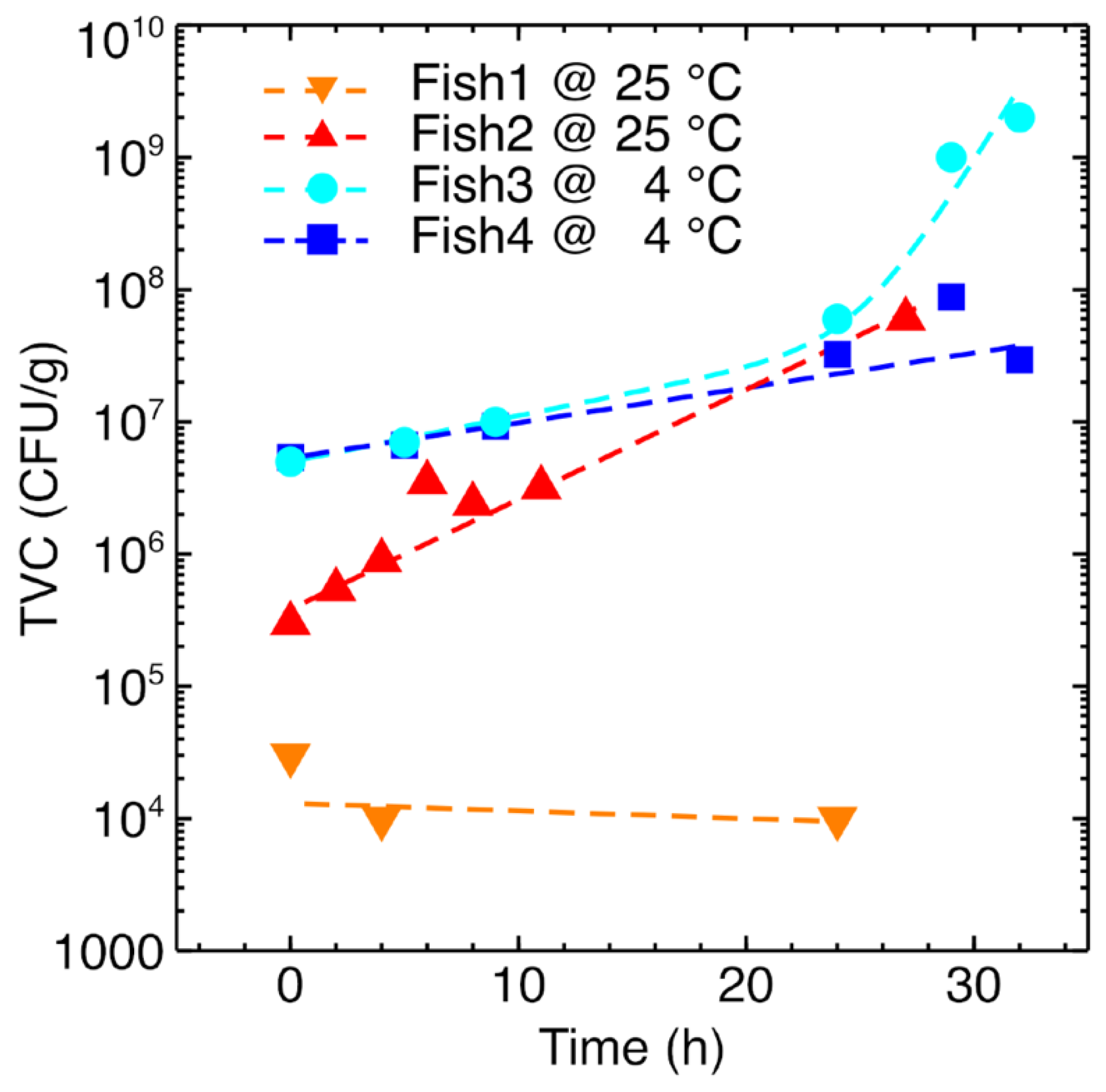
| Sample | Initial TVC (CFU/g) | Final TVC (CFU/g) | Storage and Testing Condition |
|---|---|---|---|
| Fish1 | 1 × 10⁴ | 3 × 10⁴ @ 24 h | Thermostatic chamber @ 25 °C |
| Fish2 | 3 × 10⁵ | 6 × 10⁷ @ 24 h | Thermostatic chamber @ 25 °C |
| Fish3 | 5 × 10⁶ | 2 × 10⁹ @ 32 h | Refrigerator @ 4 °C |
| Fish4 | 5 × 10⁶ | 3 × 10⁷ @ 32 h | Refrigerator @ 4 °C |
| Sterilized Water | <1 | <1 @ 32 h | Thermostatic chamber @ 25 °C |
| Air | Not performed | Not performed | Thermostatic chamber @ 25 °C |
| Air | Not performed | Not performed | Refrigerator @ 4 °C |
| Number | Retention Time (min) | Putative Identification | °# CAS | Reference Mass Spectra Similarity (%) | Samples |
|---|---|---|---|---|---|
| 1 | 5.160 | 3-methyl-1-butanol | 123-51-3 | 92 | R; F |
| 2 | 5.306 | dimethyl disulfide | 624-92-0 | 94 | R |
| 3 | 7.293 | 3-pentanone | 96-22-0 | 80 | R; F |
| 4 | 8.927 | 2,3-heptanedione | 96-04-8 | 91 | R |
| 5 | 9.259 | ethyl crotonate | 10544-63-5 | 95 | R |
| 6 | 9.626 | ethyl isovalerate | 108-64-5 | 92 | R; F |
| 7 | 10.627 | 2-heptanone | 110-43-0 | 88 | R; F |
| 8 | 11.987 | ethyl tiglate | 5837-78-5 | 93 | R |
| 9 | 12.555 | dimethyl trisulfide | 3658-80-8 | 91 | R |
| 10 | 13.024 | phenol | 108-95-2 | 96 | R; F |
| 11 | 13.340 | ethyl hexanoate | 123-66-0 | 97 | R; F |
| 12 | 15.153 | 1-undecene | 821-95-4 | 91 | R; F |
| 13 | 18.611 | indole | 120-72-9 | 87 | R |
Publisher’s Note: MDPI stays neutral with regard to jurisdictional claims in published maps and institutional affiliations. |
© 2022 by the authors. Licensee MDPI, Basel, Switzerland. This article is an open access article distributed under the terms and conditions of the Creative Commons Attribution (CC BY) license (https://creativecommons.org/licenses/by/4.0/).
Share and Cite
Zambotti, G.; Capuano, R.; Pasqualetti, V.; Soprani, M.; Gobbi, E.; Di Natale, C.; Ponzoni, A. Monitoring Fish Freshness in Real Time under Realistic Conditions through a Single Metal Oxide Gas Sensor. Sensors 2022, 22, 5888. https://doi.org/10.3390/s22155888
Zambotti G, Capuano R, Pasqualetti V, Soprani M, Gobbi E, Di Natale C, Ponzoni A. Monitoring Fish Freshness in Real Time under Realistic Conditions through a Single Metal Oxide Gas Sensor. Sensors. 2022; 22(15):5888. https://doi.org/10.3390/s22155888
Chicago/Turabian StyleZambotti, Giulia, Rosamaria Capuano, Valentina Pasqualetti, Matteo Soprani, Emanuela Gobbi, Corrado Di Natale, and Andrea Ponzoni. 2022. "Monitoring Fish Freshness in Real Time under Realistic Conditions through a Single Metal Oxide Gas Sensor" Sensors 22, no. 15: 5888. https://doi.org/10.3390/s22155888
APA StyleZambotti, G., Capuano, R., Pasqualetti, V., Soprani, M., Gobbi, E., Di Natale, C., & Ponzoni, A. (2022). Monitoring Fish Freshness in Real Time under Realistic Conditions through a Single Metal Oxide Gas Sensor. Sensors, 22(15), 5888. https://doi.org/10.3390/s22155888