1. Introduction
The brain–computer interface (BCI) is a continuously developing technology that implement the brain’s thought to manipulate external bodies without thinking through the human nerves to the hands or feet [
1,
2]. Thus, BCI systems are intended to generate new communication channels for other human parts [
3,
4]. There are two types of justifications available. One is uni-directional communication from a brain to a computer and the other is bi-direction communication between a brain and computer, as well as brain-to-brain. The current state of art technology for the BCI is bi-direction BCI technology or brain to brain interface (B2BI) [
5]. The B2BI functions via on one hand as a brain–computer interface (BCI) to retrieve messages and, on the other hand, a computer-brain interface (CBI) [
6]. The communication paths that do not go through human’s nerves could help people with physical disabilities by controlling objects, such as a wireless mouse [
7]. The signals that are generated from the human brain are used to implement the systems, and they are extremely complex; such signals are recorded in electronic system, i.e., an electroencephalogram (EEG) [
8]. In the beginning of EEG research, EEG measurement used invasive and painful methods, in which several electrodes were inserted directly into the human skin [
9]. The non-invasive methods of attaching the electrodes to the human scalps have been used because they are non-painful, user-friendly, and economical ways to obtain EEG signals [
10]. In particular, the classification of motor imagery (MI) is researched because EEG signals are shown when the right and left hands are related, respectively [
11].
In the BCI systems, raw EEG signals need to be processed with filtering, extraction, and classification techniques [
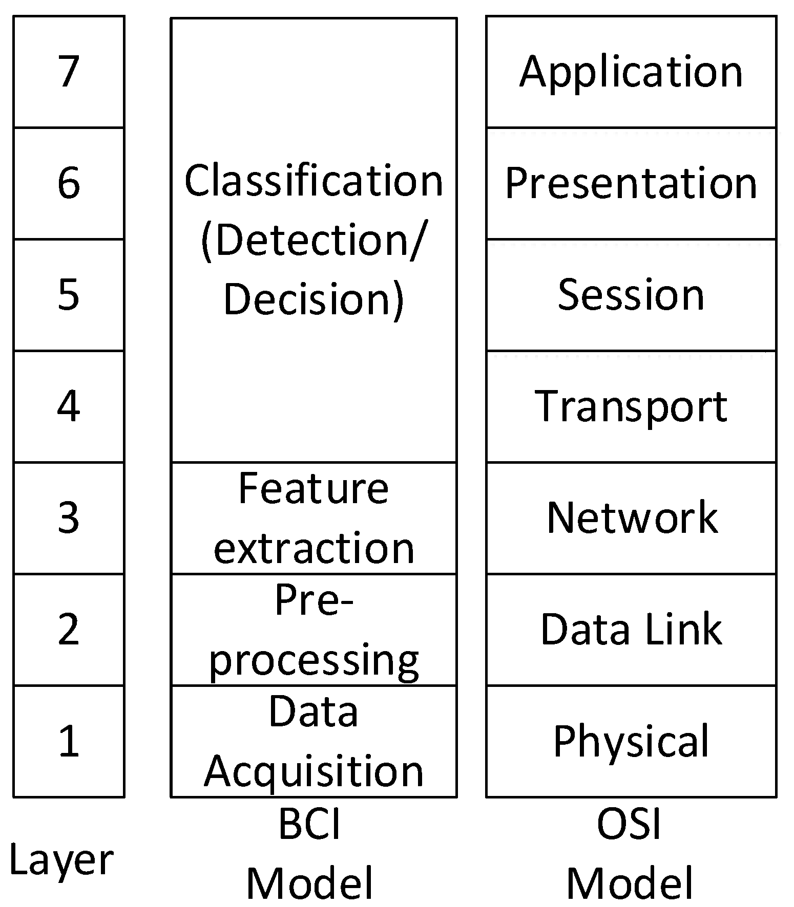
12]. We describe the whole BCI workflow based on the OSI 7-layer model; the OSI 7-layer model is a kind of the communication model. Therefore, it could be useful for readers to understand the feature extraction and classification algorithms in the signal processing workflow. In OSI 7-layer model, there are two types of disciplines. One is a datagram for a layered network hierarchy, and the other is a conceptual model for multistage processing. In the layered hierarchy model, there are the physical, medium access control, network, transport, or routing, etc. In the conceptual model for multistage processing, the focus is on multistage processing, such as the input, data acquisition, preprocessing, decision/detection, and hypothesis test. In this article, based on the previous literature of IEEE [
11], we compared the similarity between the BCI dataflow and OSI 7-layer in the conceptual model for better understanding of the signal progressing in BCIs. According to N. Khadijah et al., in the previous related work [
13], we used the open system interconnection (OSI) layer, as shown in
Figure 1. In the BCI model, we used a layer architecture staring from data acquisition (layer 1), going through pre-processing (layer 2), approaching at feature extraction (layer 3), and then ending at classification (layer 4).
In the signal processing steps, feature extraction was used; generally, a filter block is applied before feature extraction [
14,
15,
16]. There are several feature extraction methods, such as wavelet transform, short-time Fourier transform (STFT), common spatial pattern (CSP), regularized CSP (RCSP), common spatio-spectral pattern (CSSP), common sparse spectral spatial pattern (CSSSP), etc. [
8]. As a representative visualization method, short time Fourier transform (STFT), spectrogram, wavelet, etc., were used [
17]. Among those methods, the CSP is one of the most widely accepted feature extraction methods [
18]. However, the CSP method has overfitting problems when data are sparse in the domain. The CSP method is also noise sensitive, so it is difficult to classify multi-class EEG signals. Blankertz et al. focused how a CSP filter affected the EEG signals [
19]. The combination of CSP has been used by many researchers, including Lotte and Guan [
20]. Their idea was used to regularize CSP and substitute the normal CSP. The limitation is that the researchers were required to use the full set of data for the training and testing sections. The training data should have a larger number of data than the test data. The full set of data that were used, especially the test data, may lead to an overestimation in performance because all the information is being used. To classify the MI for a subject, the algorithms required the use of other subjects, as well. Therefore, the algorithms are not suitable for classifying a single subject dataset. The extended algorithm of the CSP was used by Lemm et al. [
10]. This algorithm is known as CSSP. The CSSP method introduced a delay to the system, so that the spectral filter was included in the system. The simulation results, except for six datasets, showed better accuracy than CSP.
In current EEG classification studies, linear discriminant analysis (LDA), support vector machine (SVM), deep learning, etc., were used [
21]. Deep learning (DL) is a machine learning (ML) method used in various fields, such as the voice and video processing fields [
22]. The DL works successfully on non-linear and non-stationary data, and it works efficiently even in the fields that are difficult for humans to distinguish [
23]. The convolutional neural network (CNN) is one of the DL algorithms that is widely used for data classification [
24]. Due to CNN characteristics, there are attempts to apply CNN for EEG signal classification. To use the CNN method specialized for image classification, various methods to visualize EEG signal are being studied [
25]. Visualization of these EEG signals was used to help improve the classification performance of DL models using CNN algorithms. Compared to those traditional classification algorithms, such as LDA and SVM, the deep learning model requires the use of large numbers of the dataset [
25]. Therefore, the limited numbers of the dataset need to be increased using a data augmentation technique. Considering the finite training data in BCIs, Huang et at.al proposed a data augmentation scheme via a CNN [
26]. The data augmentation has accomplished by mixing and recombining the images. Lee et al. convers the lingering problem of zero-training by utilizing a proposed CNN model connected to P300 information [
27].
In the EFA method, the calculated eigenface coefficient was used as a feature for data classification. In this case, it is possible to reconstruct the pictures using the eigenface coefficients. We proposed a novel EEG signals classification method, called quick response EFA (QR-EFA) utilizing deep knowledge in standardized and sharable QR image formulations. The QR-EFA is subjected in the EEG signal preprocessing stage. Image reconstruction or data augmentation using QR-EFA has been shown to generate QR image features suitable for CNN algorithms. To overcome the constraints, such as the trial numbers and limited BCI competition dataset in EEG, we proposed an innovative classification technique that was organically designed for EFA and CNN based on data augmentation. After learning the impulse response filter for the BCI competition IV dataset 2a (C4D2a_4c) [
28] and BCI competition III dataset 3a (D3D3a_4c) [
29], using a seven-layer simple CNN model (one input and output, one convolution, one pooling, and three fully connected), the test EEG data classification performance was measured according to the transfer function. As of today, the highest classification results for EEG 4 classes on BCI competition IV 2a is 85.4% [
1]. Based on this observation, our proposed QR-EFA method could provide higher accuracy performance of MI classification for competition dataset in BCIs.
2. Materials and Principles
The proposed EFA algorithm is a feature extraction method from EEG data that builds up neuro images, emphasizing the discriminability of classes; the feature is a kind of tool.
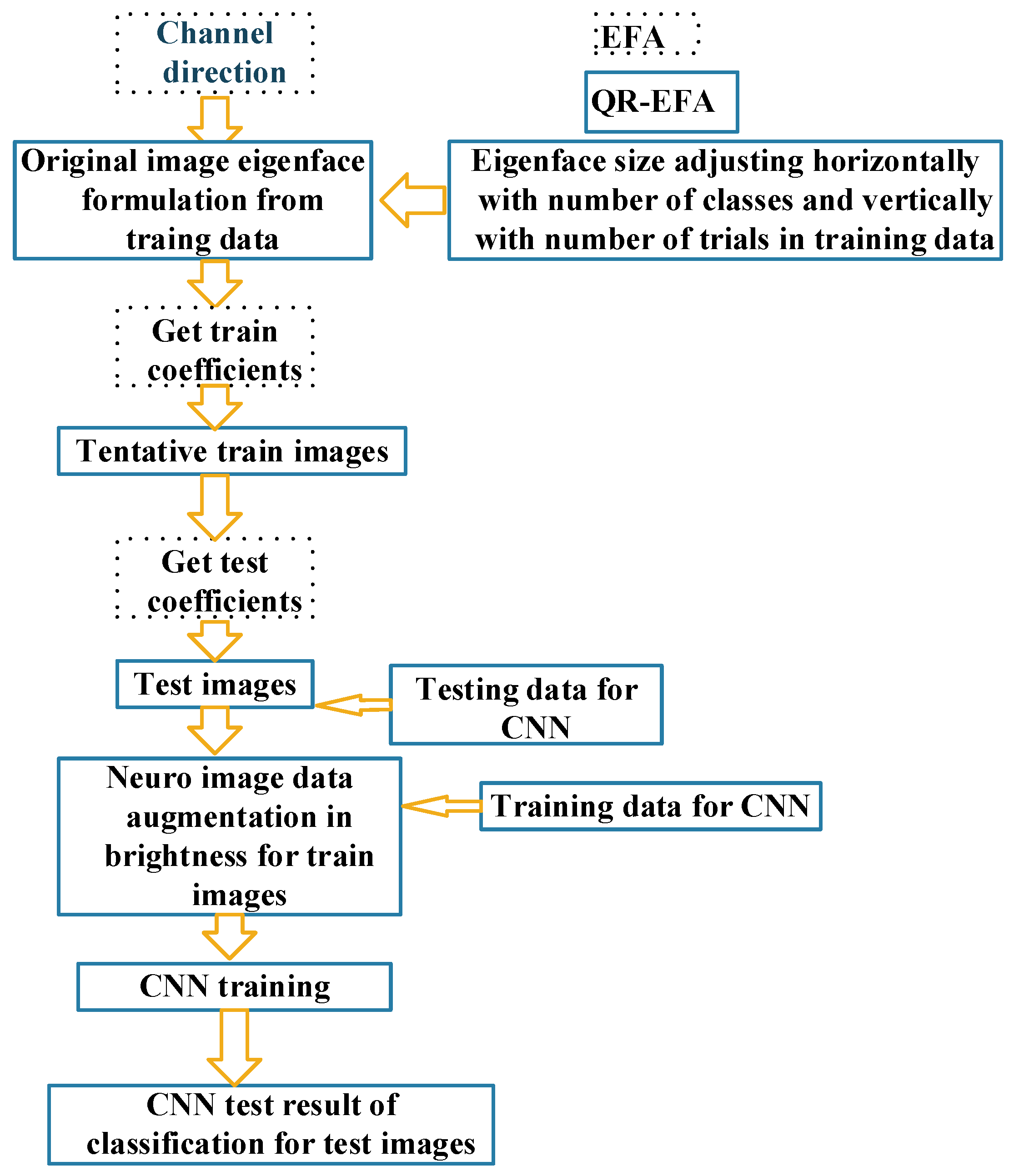
The QR-EFA method was formulated based on the previous EFA result. From egienfaces derived from the previous EFA, we will provide the description. First, the eigenface is asymmetric in horizontal and vertical directions, and the image size is excessively bigger than the size that CNN can process. Second, in BCI competition dataset, there are many discrepancies in data sizes among number of classes, trials, and subjects. Based on this fact, we proposed QR eigenface to provide a symmetrical, standardized, and sharable sizes in images. In the framework level, QR-EFA consists of the parts, such as EFA, eigenface restructuring, data augmentation, and CNN.
Figure 2 shows the relationship between the previous proposed EFA and proposed QR-EFA.
The EFA is different PCA image recognition type for dimension reduction [
30]. The fundamental EFA method is depicted in
Figure 3. The EEG data were preprocessed. As shown in steps 1–3, EEG data were converted to image data to build up eigenface. From eigenface, coefficients, which we called features, were extracted for training and testing procedures. Afterwards, the classes were classified for the next step.
Let us define the next step of the data interpretation after EFA procedure. We also used the same data interpretation techniques for classification.
Step 1: The three-dimensional (3D) converted EEG image data could be separated as time, channels, and trials. The data were recognized in each separated 3D converted EEG image data, and the generated data could be differentiated, depending on the viewpoint for each 3D direction.
Step 2: From the differentiated 3D EEG image data, the covariance matrix must be obtained. Afterwards, we could determine and build up the eigenfaces.
Step 3: The training data were projected to obtain the requested features. The dataset was composed of, or represented with, ‘
time (S)’, ‘
channels (C)’, and ‘
trials (N)’, as described in Equation (1).
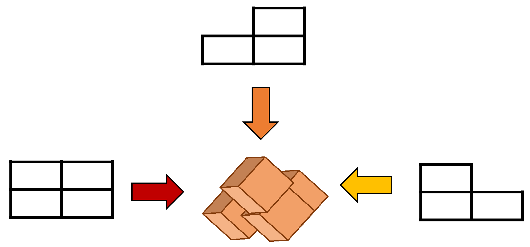
EFA is a method to obtain the differentiated EEG data with different directions. The EEG image data with the time, channels, and trials were combined into the dataset, which is an infinite number (
N) of the image data with the same manner as that illustrated in Equation (2). In other words, we consider 3D data in two-dimensional (2D) images by combining or concatenating ‘time’ and ‘channel’ data together as in
T =
SC (time × channel). In fact, the derived tentative dataset, T is composed of ‘time’ and ‘channel’ components in series. The desired dataset or image matrix was obtained by rearranging the component
T in horizontal direction and component
N in vertical direction as shown in
Figure 4. Consequently, Equation (2) shows the final dataset or 2D images.
The eigenface was then obtained from differentiated 3D EEG image, and newly obtained image data
Φ and value
Ψ need to be calculated.
The covariance matrix extracted from the differentiated 3D EEG image data without the mean value is obtained in Equation (4).
Let us define the eigenvectors of
X with eigenvalues of
L of the covariance matrix
C after solving the following equation
CX =
kX. Among the vectors extracted from this matrix, the
k vectors were chosen. The eigenfaces must be extracted with only training eigenface
Гtrain. Subsequently, the training features were extracted from the training eigenface and data. The extracted eigenface coefficients were projected in Equation (5).
The weight coefficient
Ωtrain was obtained to be a training feature. Equation (6) shows how to obtain the feature coefficient
Ωtest. The eigenspace was trained, and the EEG test data can be classified as shown in Equation (6).
4. Experimental Results
The QR codes are widely used for quick response as matrix barcodes. Just as with QR codes, we also obtained the images, so we called them QR images. After performing QR image data, we need further steps. In obtaining QR images for training and testing images, there are three factors to consider for better classification, in order to have accurate, robust, and reliable results. First, let us define some terminologies, such as the domain-wise similarity among domains, trial-wise similarity among trials, and subject-wise similarity among subjects. Domain-wise similarity is the degree of similarity that indicates some common characteristics on the eigenfaces between the training and testing domains. Trial- and subject-wise similarity were degrees of similarity among trials and subjects, respectively. We could recognize the similarity from QR images. Our proposed QR-EFA algorithm maximizes the similarities, with the respect to domains, trials, and subjects. As result, it could generate unique features per domain, so it is possible to discriminate the classes efficiently.
The background regarding EEG datasets from BCI competitions needs to be explained. To validate the proposed method, we used two EEG datasets, such as the BCI competition III dataset 3a (C3D3a_4C) and BCI competition IV dataset 2a (C4D2a_4C), for four classes. Specifically, C3D3a_4C is dataset from three subjects or participants, and C4D2a_4C is dataset from nine subjects, which are the off-line, publicly available, and open accessible dataset of the BCI competition database. Hence, this article focuses on the C3D3a_4c and C4D2a_4C.
Table 1 shows the detailed number of trials per subject for the C3D4a_4C used in this article.
The detailed information of the property for C3D3a_4C is given as follows (
Box 2).
Box 2. The detailed information of the property for C3D3a_4C.
comment1: ‘dataset: C3D3a_4C’
date: ‘2021.12.28’
madeby: ‘4C’
affiliation: ‘KNIT’
window: ‘offset: 3.5, length: 2’
subject: ‘subject #: 1’
prefiltering: ‘off’
s: 250 (sample/sec)
c: [1 × 60 cell]
x: [500 × 60 × 180 double]
y: [1 × 180 double]
The MI classification EEG images extracted with QR-EFA were classified for C3D3a_4C. The data augmentation using Gaussian distribution was used for sufficient training of the ML model and prevention of overfitting. From 10,800 augmented training images, which come from the data augmentation of the original QR neuro images, in brightness and without data augmentation, a total of 2592 non-augmented test images were used. As a result of the final classification experiment, the accuracy was obtained for the test dataset of 2592 sheets, as shown in
Table 2.
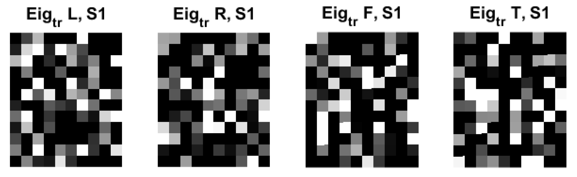
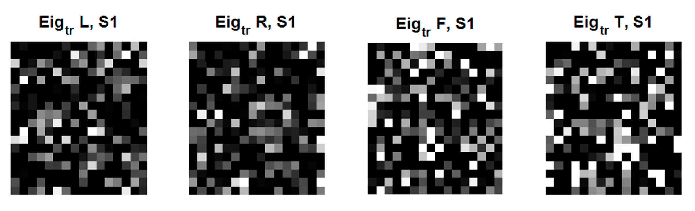
Figure 7 shows the examples of eigenfaces, formulated based on the QR code. Although there are lots of QR-eigenfaces are available, we will confine only a small number of eigenfaces, considering the number of classes and trials among the subjects. We chose the eigefacecs reflecting the number of classes. We designed the first to left, second, right, the third to feet, and the last to tongue classes. However, the order is subject to change as the supervisory learning constrictions. This type of decision is related to the choice regarding the approach between the supervised and unsupervised learning.
Thus far, we obtained the training coefficients by projecting the training images to the QR-eigenfaces and testing the coefficients by projecting the testing images to the QR-eigenfaces. The next step is to conceive of new QR images for training and testing the dataset. Subsequently, linear combinations of the QR eigenfaces, weighted by the relevant coefficients, were used as QR images for training and testing data.
During the data augmentation process for overcoming the limited dataset problem in the BCI competition, we modified the brightness of the recovered images based on the Gaussian noise contamination equation. Although the grayscale and quantized images from the first to last appear similar, the real binary values of the images are different and unique, and they can be used for classification. Because of ML or AI paradigm considerations, a sufficiently large number of training images are needed to train CNNs and fine-tune the logic. However, as the BCI training dataset and its QR images are finite and limited, we need to amplify or diversify them by utilizing data augmentation in the brightness direction.
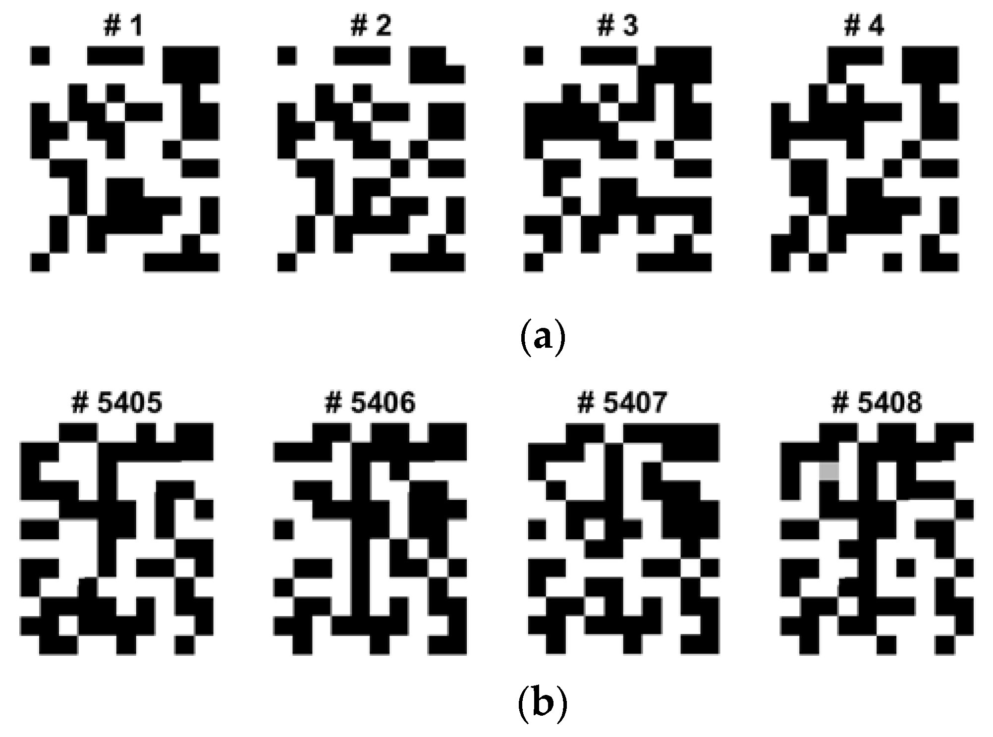
Figure 8 shows one of the EFA QR code implementation results after the brightness data augmentation. Among four classes, considering its dominance and the activation region of the brain, we only selected and data augmented four QR training images for the left and tongue classes, as shown.
Because the BCI data are random signals, they must be treated in statistical signal-processing domains.
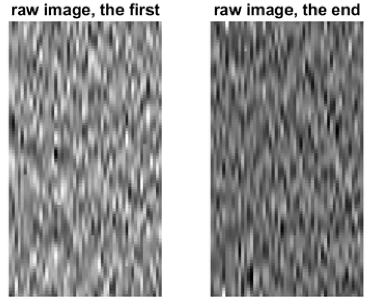
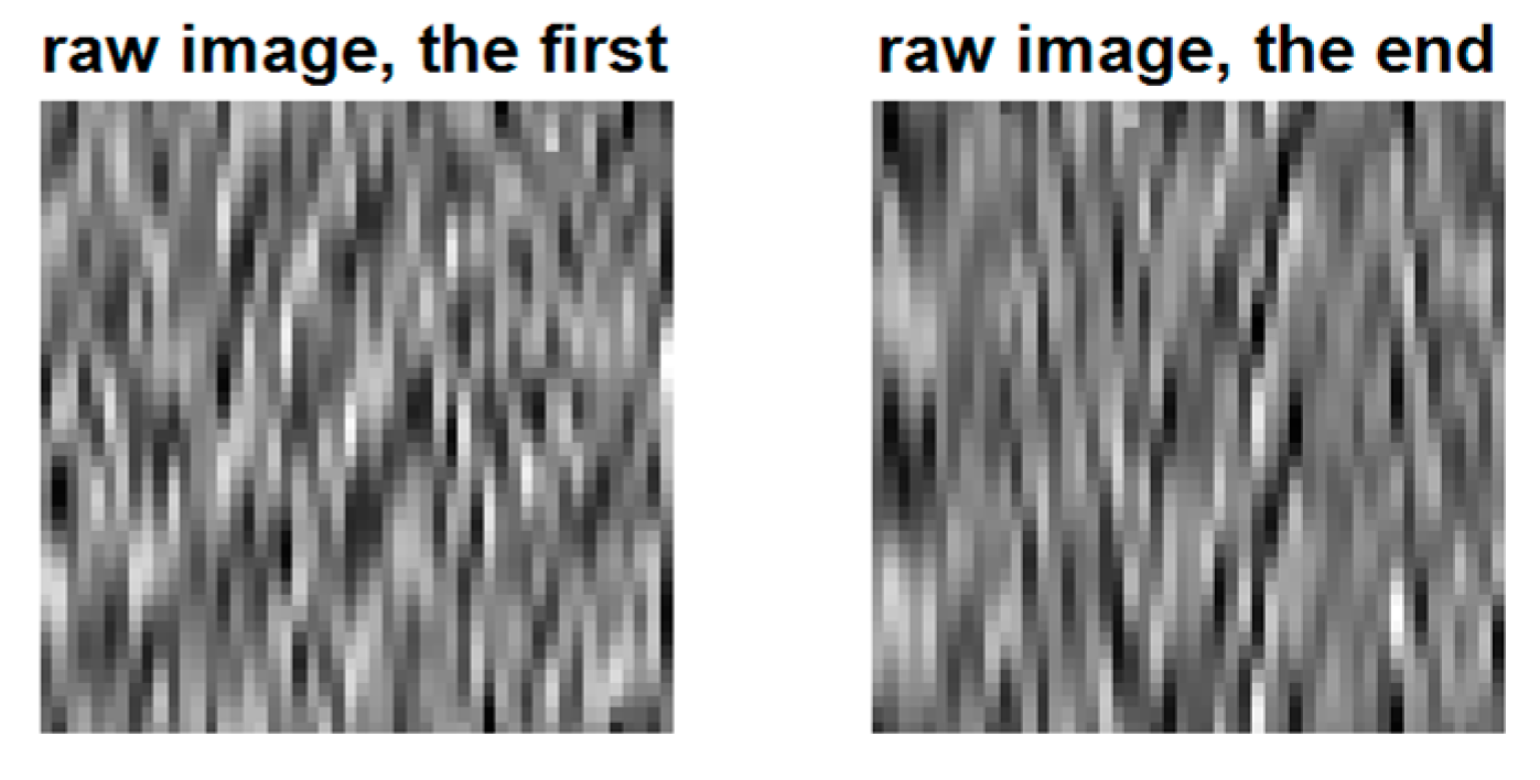
Figure 9 shows the typical neuro raw images considered for the QR-EFA. The left image is for the first trial, and the right image is for the last trial.
Based on the QR-eigenfaces for left, right, feet, and tongue, we proposed considering domain-, trial-, and subject-wise similarities. The detailed considerations are as follows. First, subject-wide similarities among the subjects were checked. Second, domain-wise similarity between the training and testing domains was considered. Finally, a trial-wise similarity was investigated among the trials.
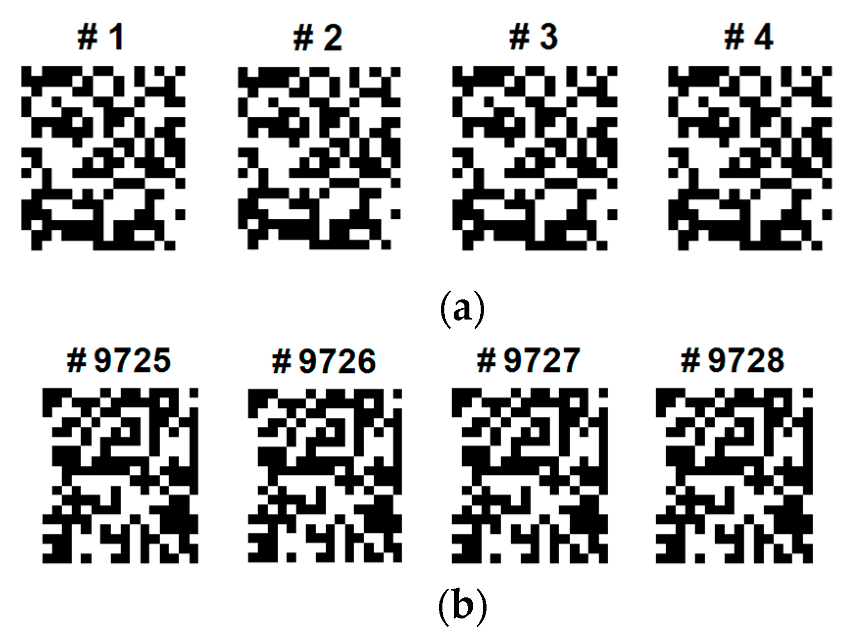
Figure 10 shows the domain-wise similarity between the training and testing domains for subject 1. Considering their importance and the degree of information, only the QR images for subject 1 and trial 1 are shown among training or testing data and several trials. There are many similarities between training and testing QR images. We observed the trial-wise similarity of QR images between the first and last trials for subject 1. We also examined subject-wise similarity of QR images between subjects in the same first trial. It was confirmed that QR-EFA maximizes the three proposed similarities in domain, trials, and subjects.
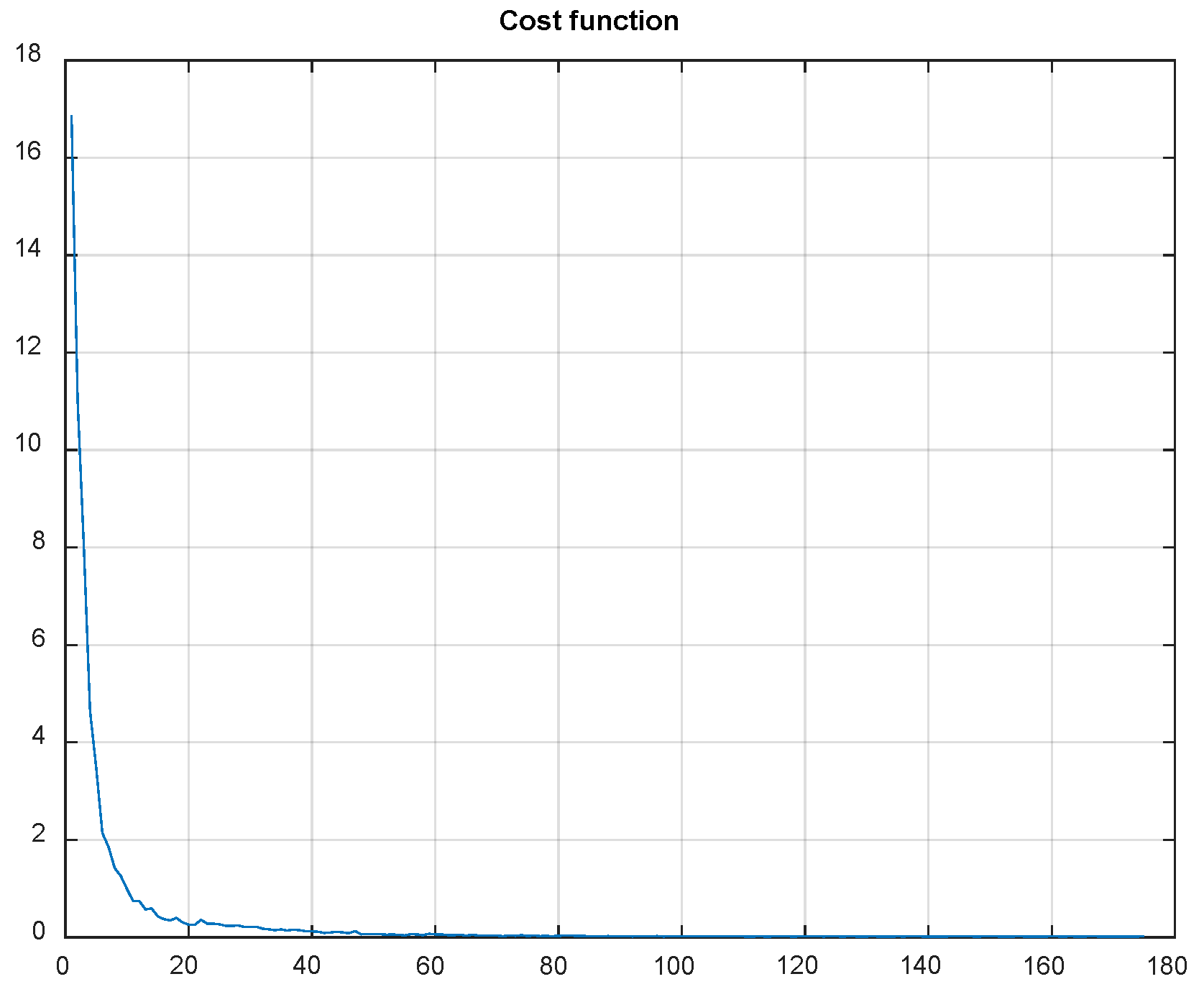
Using QR-EFA, a sample output of the CNN testing results for BCI competition III dataset 3a (C3D3a_4C) is shown in
Figure 11. As the number of epochs increases during simulations, the cost or loss function decreases and reaches a limit.
The MATLAB code for a sample mean of C3D3a_4C data and its confidence interval, when the sample size n = 10 is, as follows (
Box 3).
Box 3. The MATLAB code for a sample mean of C3D3a_4C.
% result set #1
x1(1) = 0.907143; x1(2) = 0.795238; x1(3) = 0.802381; x1(4) = 0.980952;
x1(5) = 0.919048; x1(6) = 0.859524; x1(7) = 0.921429; x1(8) = 0.904762;
x1(9) = 0.909524; x1(10) = 0.821429;
% result set #2
x1(1) = 0.857143; x1(2) = 0.930952; x1(3) = 0.928571; x1(4) = 0.926190;
x1(5) = 0.945238; x1(6) = 0.864286; x1(7) = 0.871429; x1(8) = 0.783333;
x1(9) = 0.928571; x1(10) = 0.952381;
SD1 = std(x1); % Standard deviation (SD)
SE1 = SD1/sqrt(length(x1)); % Standard error(SE)
ts1 = tinv([0.025 0.975],length(x1)−1);
% T-value/score for 95% CI (2.26)
CI1 = mean(x1) + ts1 * SE1;
% Confidence Intervals
>>mean(x1)
Ans = 0.8821
>>std(x1)
ans = 0.0602
>>CI1 % Confidence_Interval
CI1 = 0.8390 0.9252
>>CI1(2)-mean(x1) %Confidence Interval
Ans = 0.0431
The computation, simulation, verification, and validation on the proposed scheme requires considerations of the confidence interval for the given number of trials (n) and variance or standard deviations. Based on the nature of random seeds in statistical signal processing, we consider a 95% confidence interval, due its variance and spread for data augmentation, CNN layer initiations for kernel filters, and QR-eigenface selections for training images.
From the above results, with a 95% confidence interval, the sample mean was estimated to be 0.88, with a confidence interval of 0.0431. Note that, in this case, the Student’s
t-distribution is applicable for calculating the confidence interval and sample variance (
s2), because we do not have information regarding the variance or standard deviation (SD) of the population distribution in BCI datasets (C3D3a_4C or C4D2a_4C both).
Table 3 shows the 10 simulation results, as the random seeds changes uniformly for statistically justification for confidence interval.
To calculate a 95% confidence interval for the sample mean
μ, an estimated coefficient value 2.26 was used [
35]. Thus, the mean and confidence interval of accuracy were 88.21% ± 6.02%, with the confidence interval of 4.31, i.e., (83.90, 92.52). Consequently, the probability for the same mean under the 95% confidence interval is given by Equation (8). For a comparison, the latest and best classification accuracy reported thus far for EEG four classes on BCI competition IV 2a was 85.4 [
31].
Then, we compute the confidence interval using Equation (9).
To validate and verify QR-EFA in a real dataset, with a comparison to C3D3a_4C, the next section is for the result of C4D2a_4C.
Table 3 shows the number of trials per subjects for C4D2a_4C. The C4D2a_4C dataset is composed of nine subjects and the predefined number of experimental trials. The number of trials for left, right, foot, and tongue classes in the C4D2a_4C dataset, composed of nine subjects and the predefined number of experimental trials, was 72.
The detailed information of the property for C4D2a_4C is given as follows (
Box 4).
Box 4. The detailed information of the property for C3D2a_4C on MATLAB.
comment1: ‘dataset: C4D2a_4C’
date: ‘2021.02.12’
madeby: ‘4C’
affiliation: ‘KNIT’
window: ‘offset: 3.5, length: 2’
subject: ‘subject #: 1’
prefiltering: ‘off’
s: 250 (sample/sec)
y: [1 × 288 double]
x: [500 × 22 × 288 double]
c: [22 × 1 cell]
Using the designated CNN model, which is depicted in
Figure 7, MI classification EEG images extracted with QR-EFA were classified for C4D2a_4C. The accuracy was obtained for the test dataset of 2592 sheets, as shown in
Table 4.
In
Figure 12, the eigenfaces has been formulated. The eigenfaces reflecting the number of classes were selected. Considering a supervisory learning limitation, we designed the first to left, second, right, third to feet, and last to tongue classes.
The training coefficients by projecting the training images to the QR-eigenfaces and testing coefficients by projecting the testing images to the QR-eigenfaces were obtained. The next step is to conceive of new QR images for the training and testing dataset. Afterwards, we will perform a liner combination of the QR-eigenface, depending on the relevant coefficients. The results of the linear combination were the QR images for the training and testing data.
Figure 13 shows the results after brightness data augmentation in the brightness direction. Among four classes, the selected and data augmented images for left and tongue classes are shown.
Figure 14 shows the typical neuro raw images. The left image was of the first trial and the right was of the last trial for subject. First, we need to check the subject-wide similarity among subjects. Secondly, we check the domain-wise similarity between training and testing domain. Finally, we check the trial-wise similarity among trials.
Figure 15 shows the domain-wise similarity between training and testing domain for subject 1 and trial 1. There were also similarities between the training and testing images. Hence, we also maximized the similarities in the directions of domain, trials, and subjects.
In summary, it is clear that QR-EFA guarantees a distinguishable and discriminative feature per class, as well as a higher similarity, with respect to domain-, trial-, and subject-wise similarities. This unique novel scheme accelerates the improved accuracy in CNNs. With QR-EFA, a sample output of CNN testing results for in C4D2a_4C is provided in
Figure 16. It also shows that the cost function reached the limit.
The MATLAB code for a sample mean of in C4D2a_4C data and its confidence interval, when the sample size n = 10 is, as follows (
Box 5).
Box 5. The MATLAB code for a sample mean of in C4D2a_4C data.
% result set #1
x1(1) = 0.966435; x1(2) = 0.976852; x1(3) = 0.984954; x1(4) = 0.971065;
x1(5) = 0.969136; x1(6) = 0.983025; x1(7) = 0.986883; x1(8) = 0.985725;
x1(9) = 0.984182; x1(10) = 0.978395;
SD1 = std(x1); % Standard deviation (SD)
SE1 = SD1/sqrt(length(x1)); % Standard error(SE)
ts1 = tinv([0.025 0.975],length(x1)−1); % T-value/score for 95% CI (2.26)
CI1 = mean(x1) + ts1 * SE1; % Confidence Intervals
>>mean(x1)
Ans = 0.9787
>>std(x1)
ans = 0.0075
>>CI1 % Confidence_Interval
CI1 = 0.9733 0.9840
>>CI1(2)-mean(x1) %Confidence Interval
Ans = 0.0054
Table 5 shows the 10 simulation results, as the random seeds changes uniformly for statistically justification for confidence interval.
From the above results, with a 95% confidence interval, we obtained a range of estimates for a sample mean (0.98), and the confidence interval was 0.0054. The mean and confidence interval of the accuracy was 97.87 ± 0.0075%, with a confidence interval of 0.0054, i.e., (97.33, 98.40). The latest and best classification result is shown below. Then, we compute the confidence interval using Equation (10).
5. Conclusions
In this study, we proposed the QR-EFA method for efficient motor-imaginary (MI) EEG classification and showed that the EEG signal, when converted into a standardized and sharable QR image, can be classified when using a simple CNN. To obtain a unique feature per class, EEG signal data can be utilized with the concepts of domain-, trial-, and subject- similarities. The EEG data measured from several subjects were used using the BCI competition 3 dataset 3a (C3D3a_4C) and BCI competition 4 dataset 2a (C4D2a_4C). Through QR-EFA method, the EEG signal was converted into EEG QR image, as formed with the EFA method, and a data augmentation technique was applied to solve the limited EEG image problem.
For optimum and best classification performance, QR-EFA maximizes the proposed domain-, trial-, and subject-wise similarities. As far as we are concerned, none of the literature in BCIs has considered the domain-, trial-, and subject-wise similarities so far. Based on this observation, our proposed QR-EFA method was used to maximize the three similarities in the directions of domains, trials, and subjects. Using a simple seven-layer CNN model, data classification results showed an exceptional and remarkable accuracy of 97.87% ± 0.75, with a confidence interval of 0.54, i.e., (97.33, 98.40) for the C4D2a_4C and 88.21% ± 6.02, with a confidence interval of 4.31, i.e., (87.90, 92.52) for the C3D3a_4C. Unlike the CSP method, which is only robust in the original two-class classification, the proposed QR-EFA method is applicable to the classification of two multi-classes of EEG signal; hence, it definitely advantages from the use of the QR-EFA algorithm. Because the QR-EFA method extracts classification features and generates EEG QR images that are well-differentiated between classes, it is suitable as training and testing input images for further ML process and can greatly contribute to classification performance improvement.
Because the ML technique for image classification is becoming stronger with the development of better performance models and hardware performance, QR-EFA’s flexible EEG conversion method or frameworks, which should be applied to non-motor imaginary (MI), such as word thinking, emotion detections, arithmetic calculation operations, and multi-class classification, will be developed in the future. The application to a larger number of classes, such as five or six categories, will be applied, with slight extensions in time.


