
Feedforward Control of Piezoelectric Ceramic Actuators Based on PEA-RNN


Abstract
:1. Introduction
2. Performance Test and Related Structure
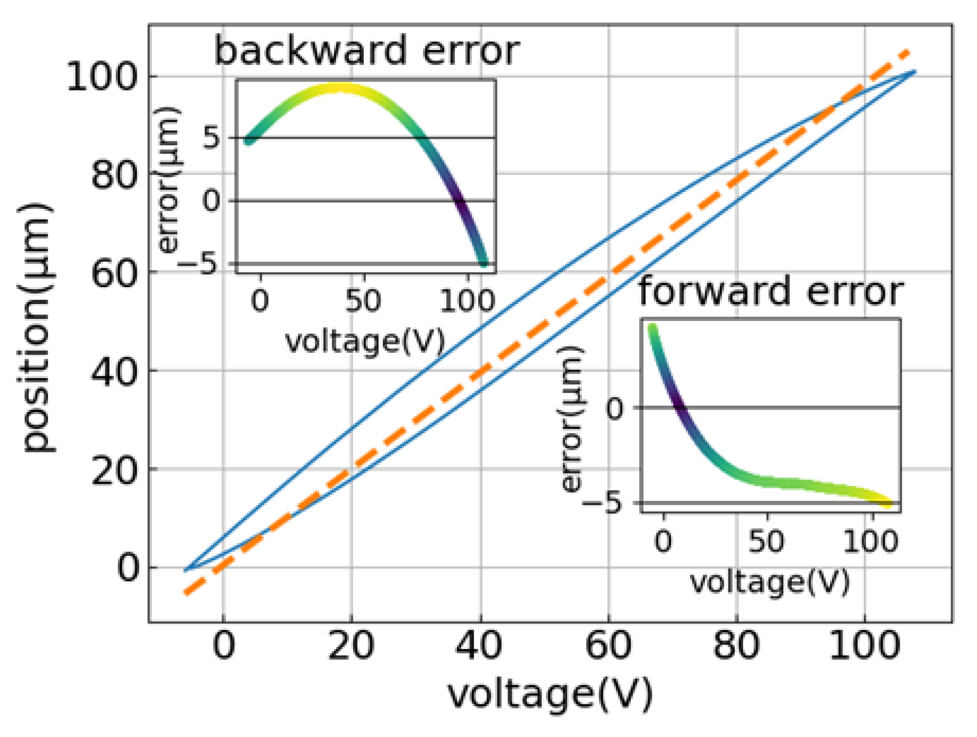
2.1. Piezoelectric Ceramic Hysteresis Loop
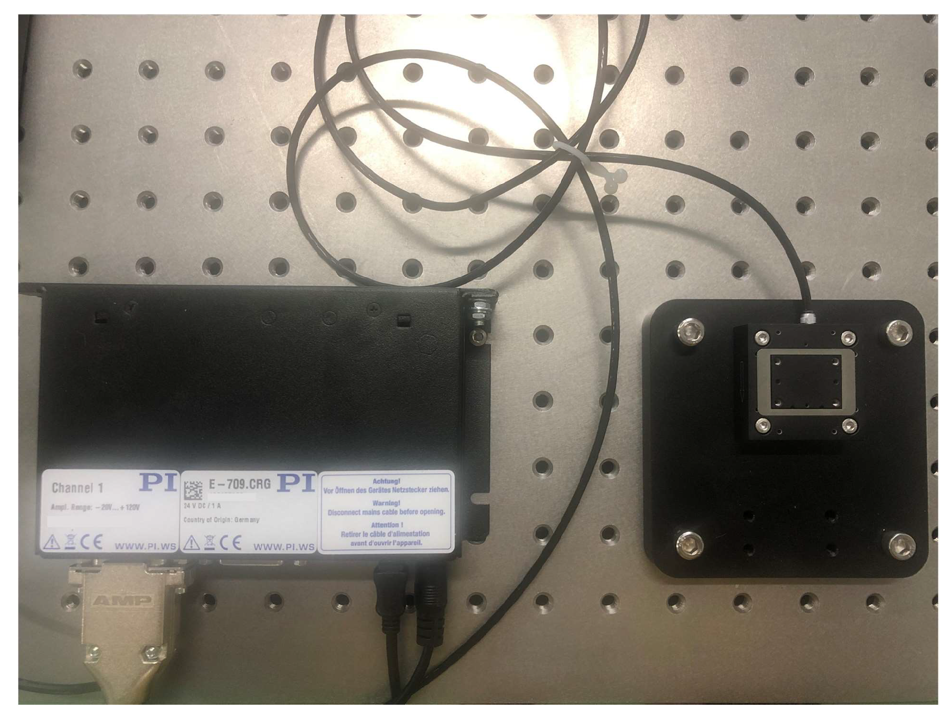
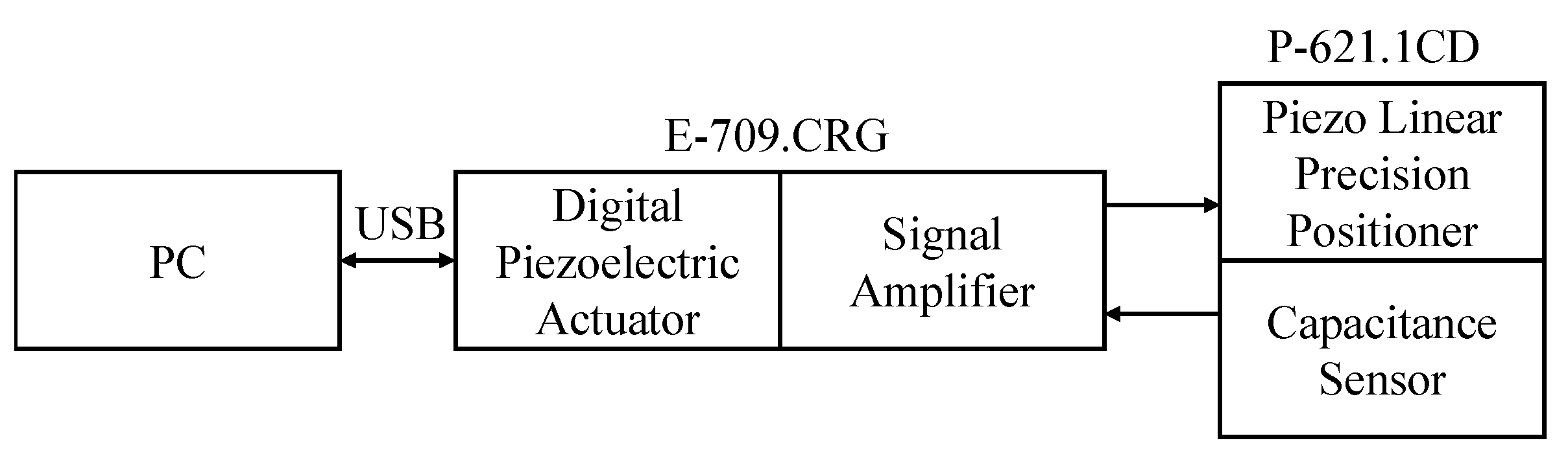
2.1.1. Experimental Platform
2.1.2. Primary and Secondary Hysteresis Loops
2.1.3. Hysteresis Loop Model
2.2. Network Structure
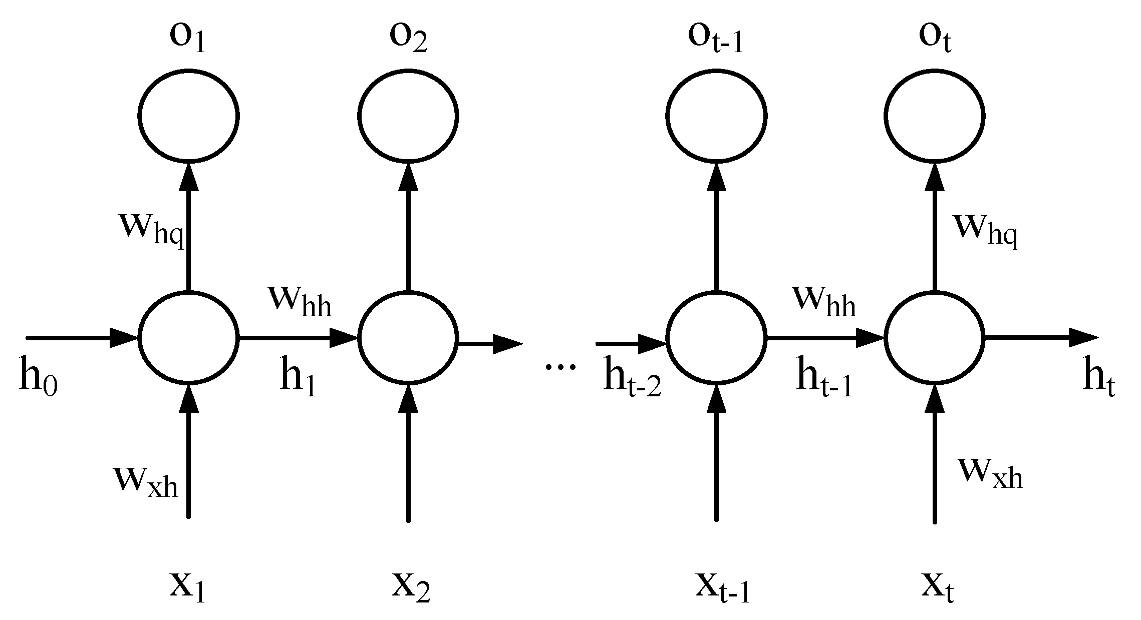
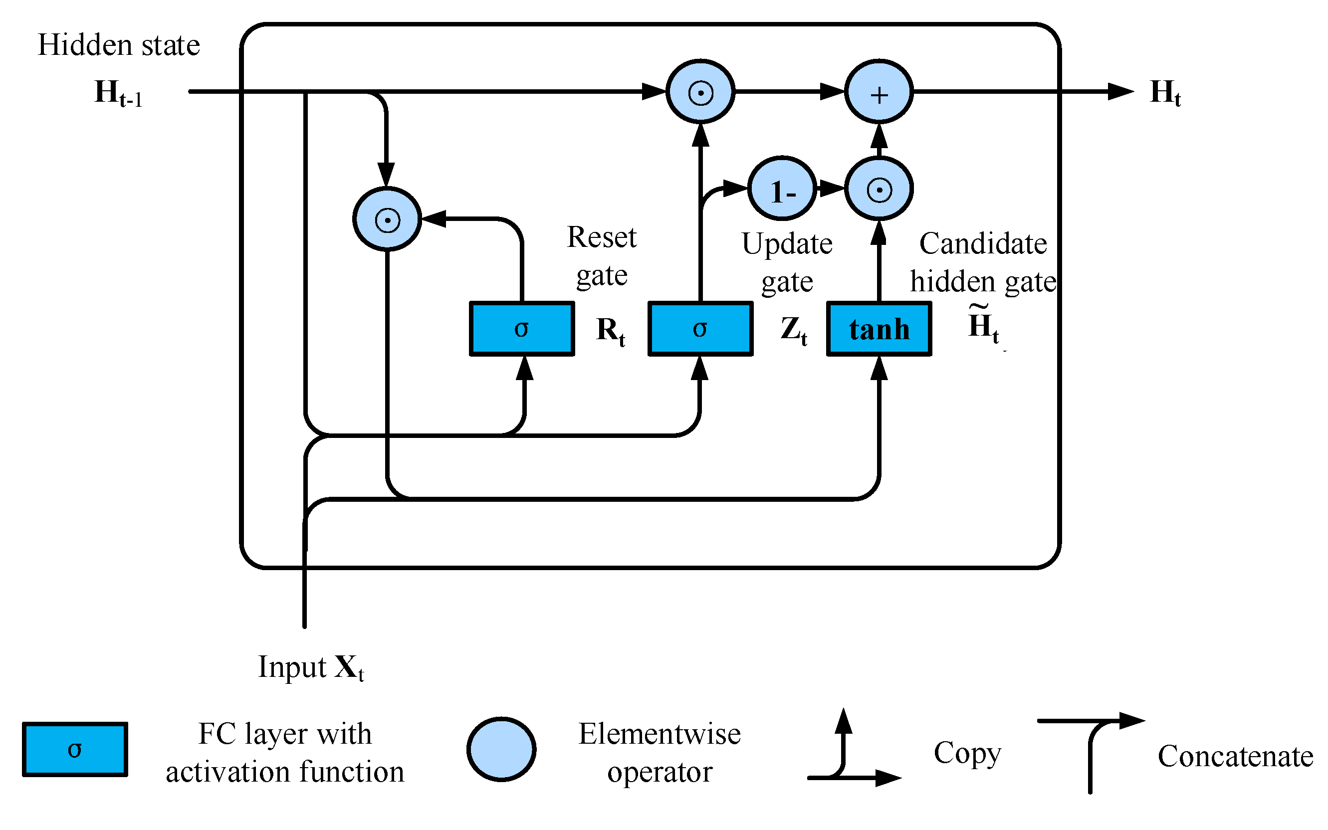
2.2.1. Recurrent Neural Network (RNN) and Gated Recurrent Unit (GRU)
- Reset gate helps capture short-term dependencies in the sequence;
- Update gate helps capture long-term dependencies in the sequence.
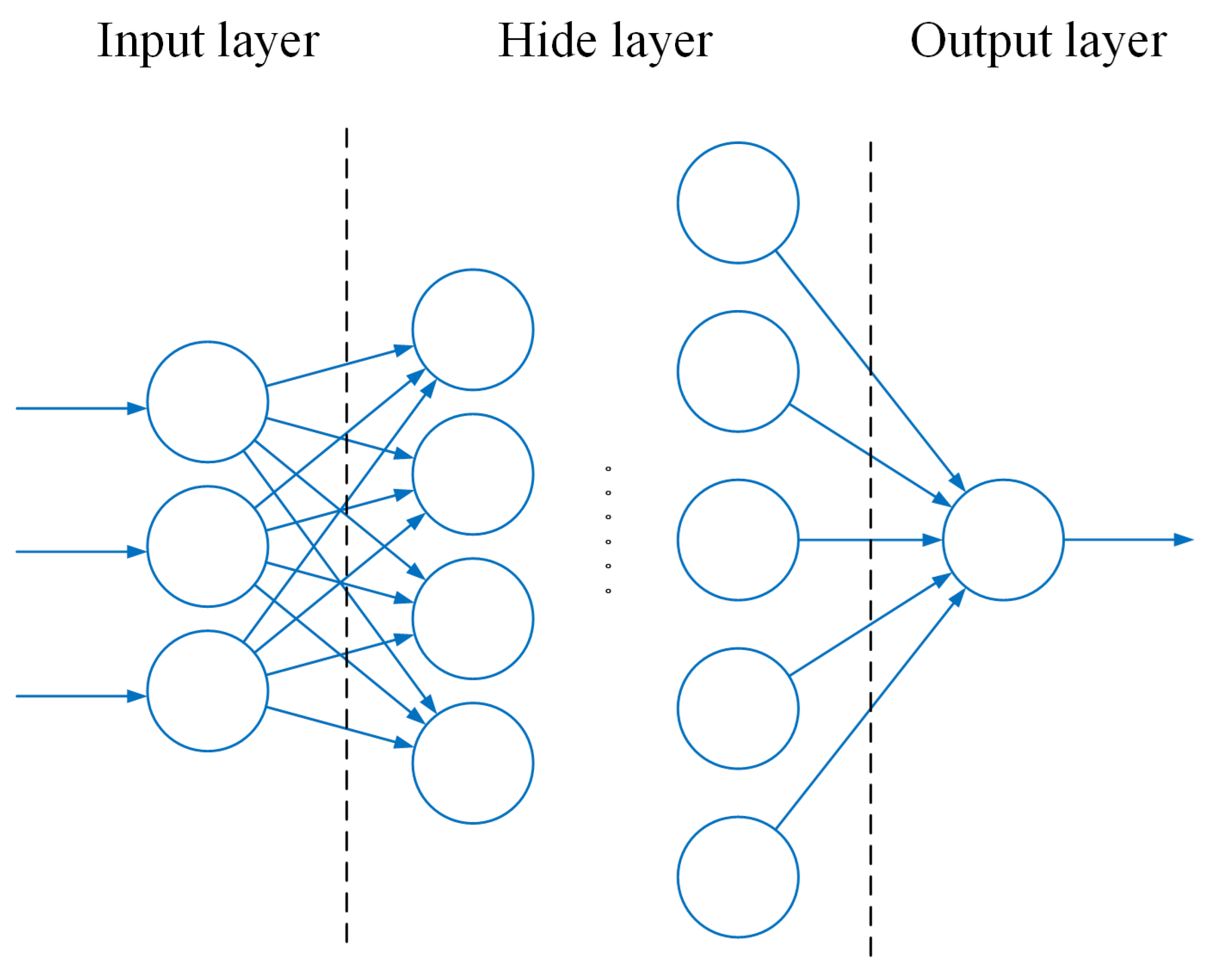
2.2.2. Multilayer Perceptron (MLP)
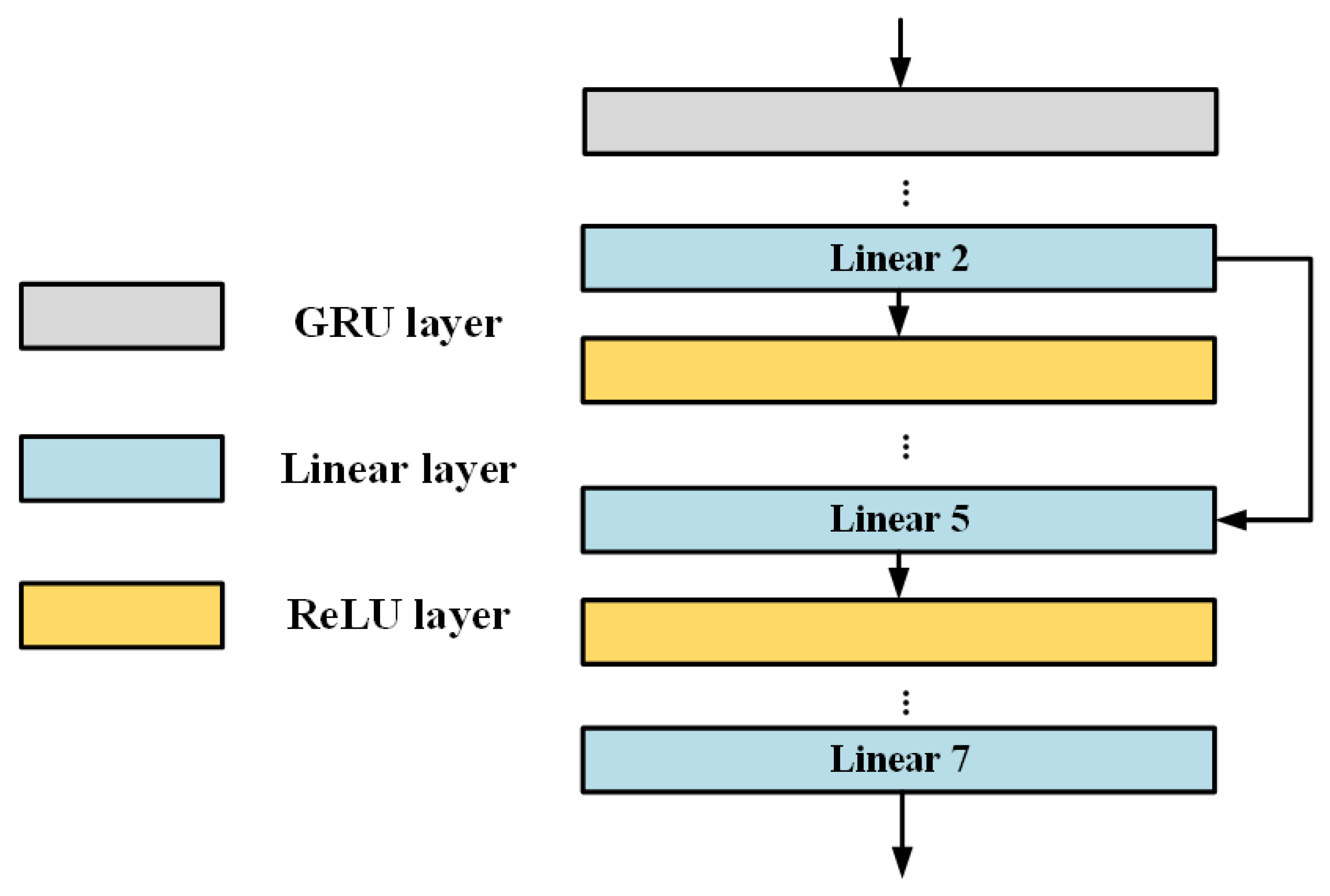
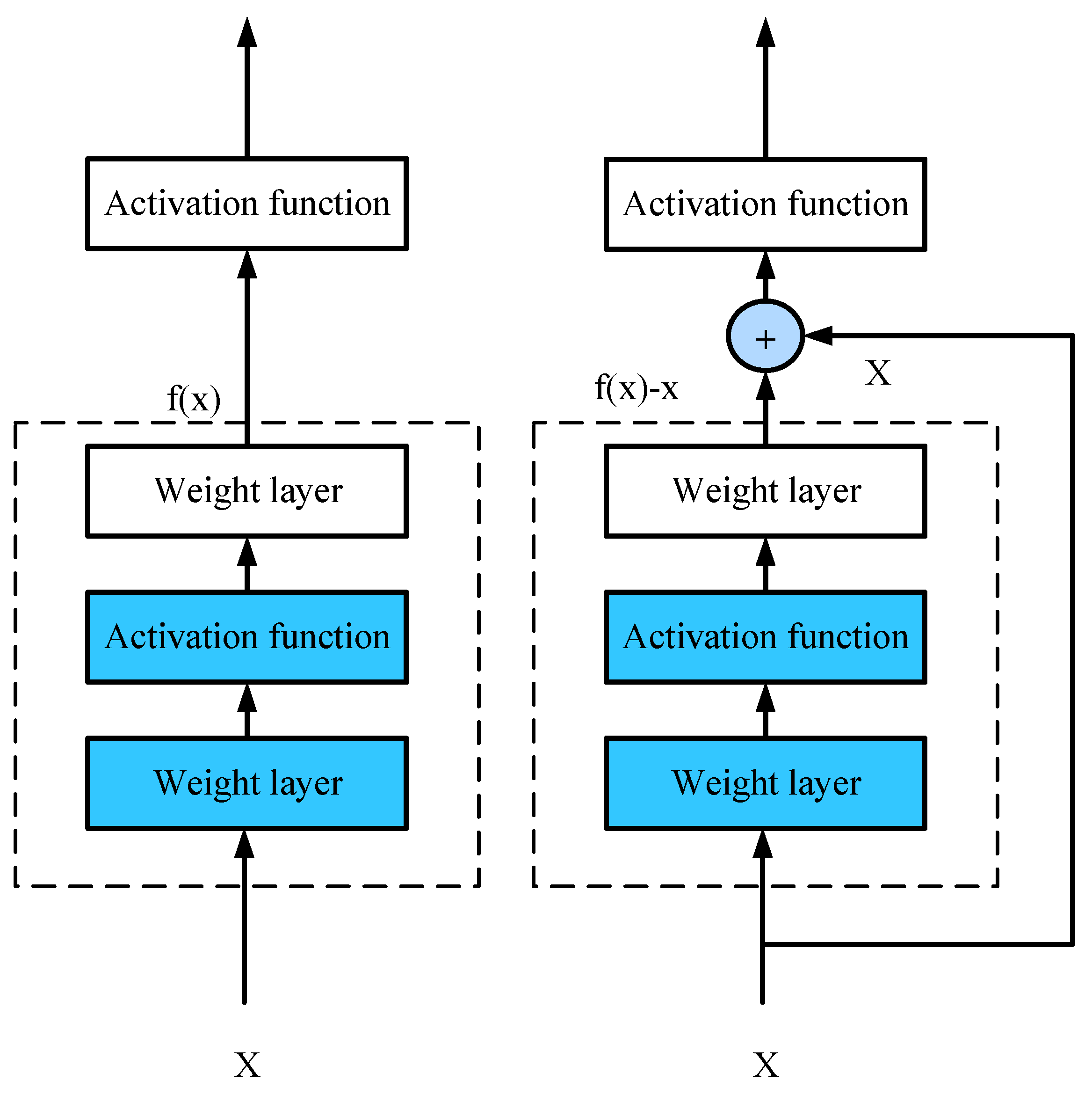
2.2.3. Residual Connection
3. Training and Application of PEA-RNN
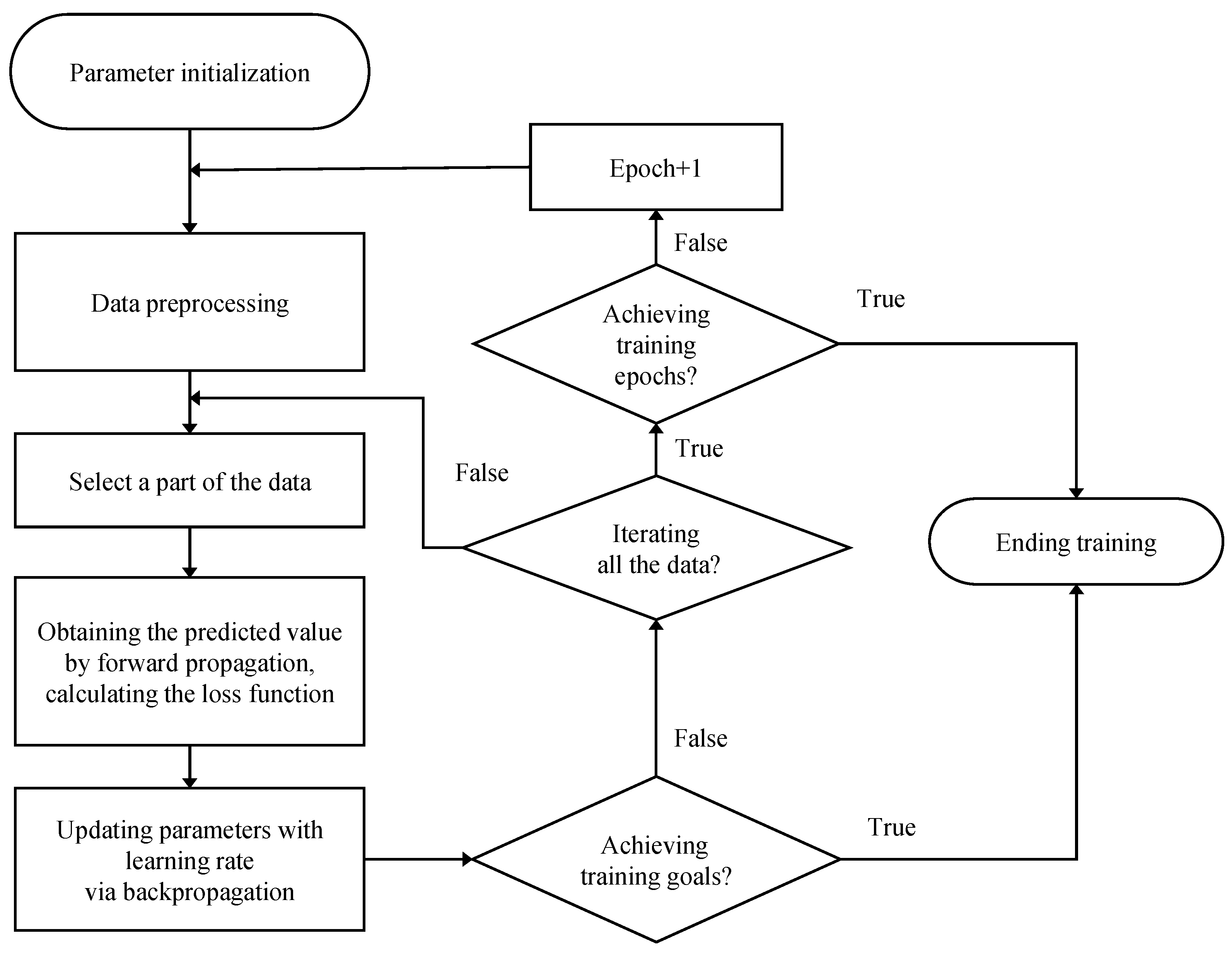
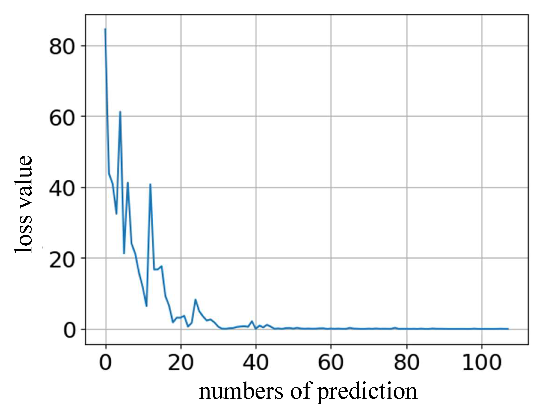
3.1. Network Training
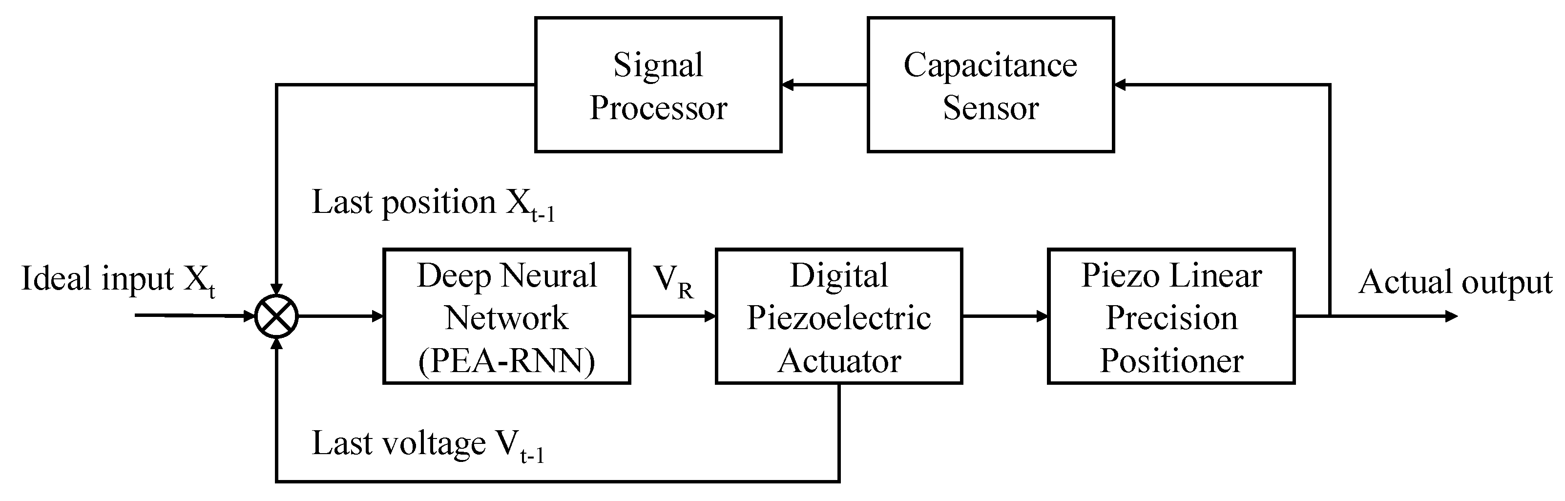
3.2. Network Application
3.2.1. The Overall Structure of PEA-RNN
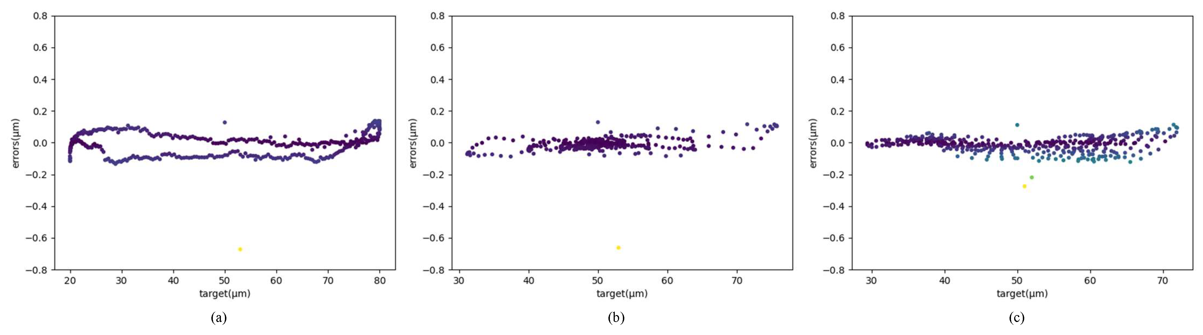
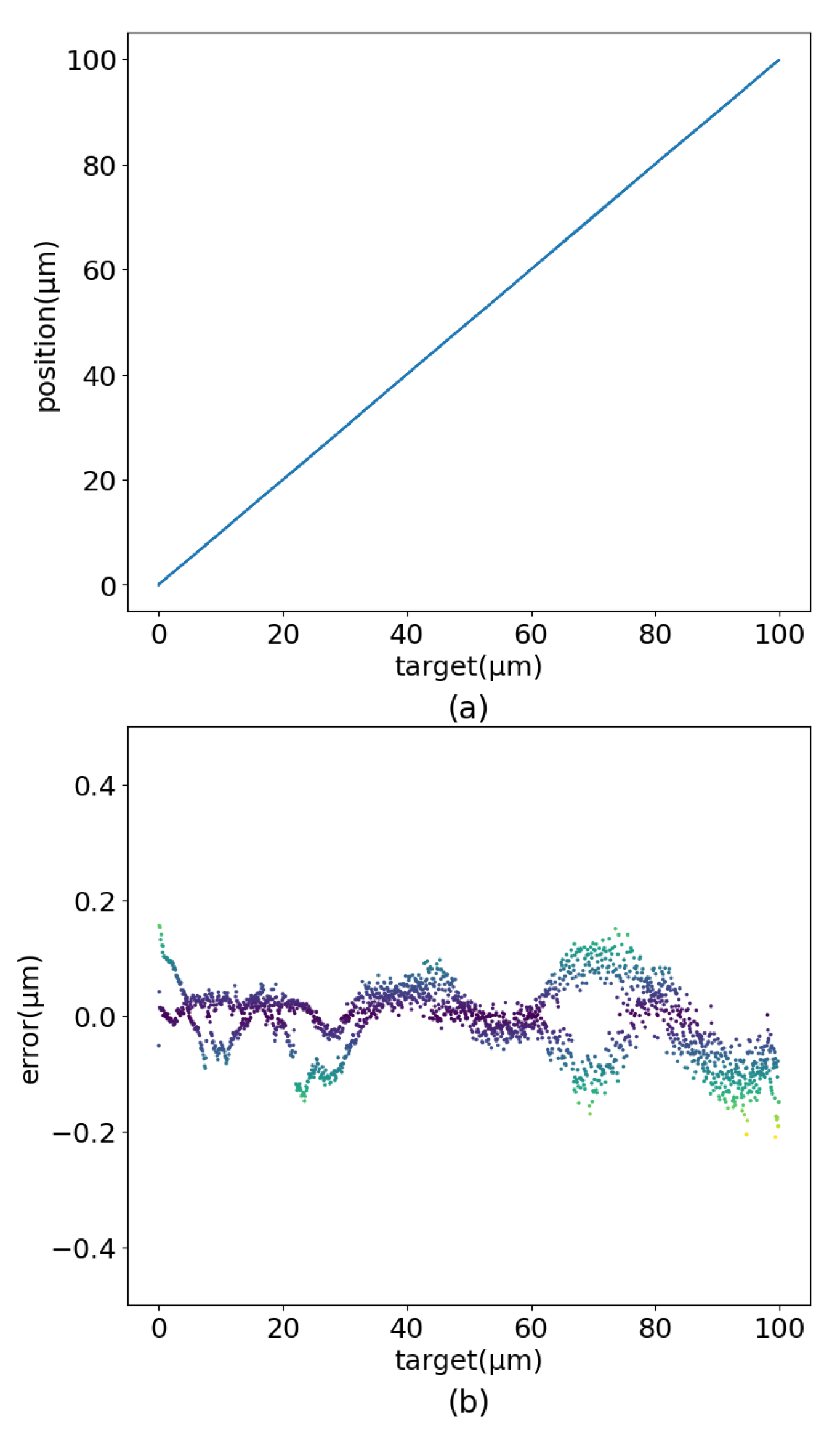
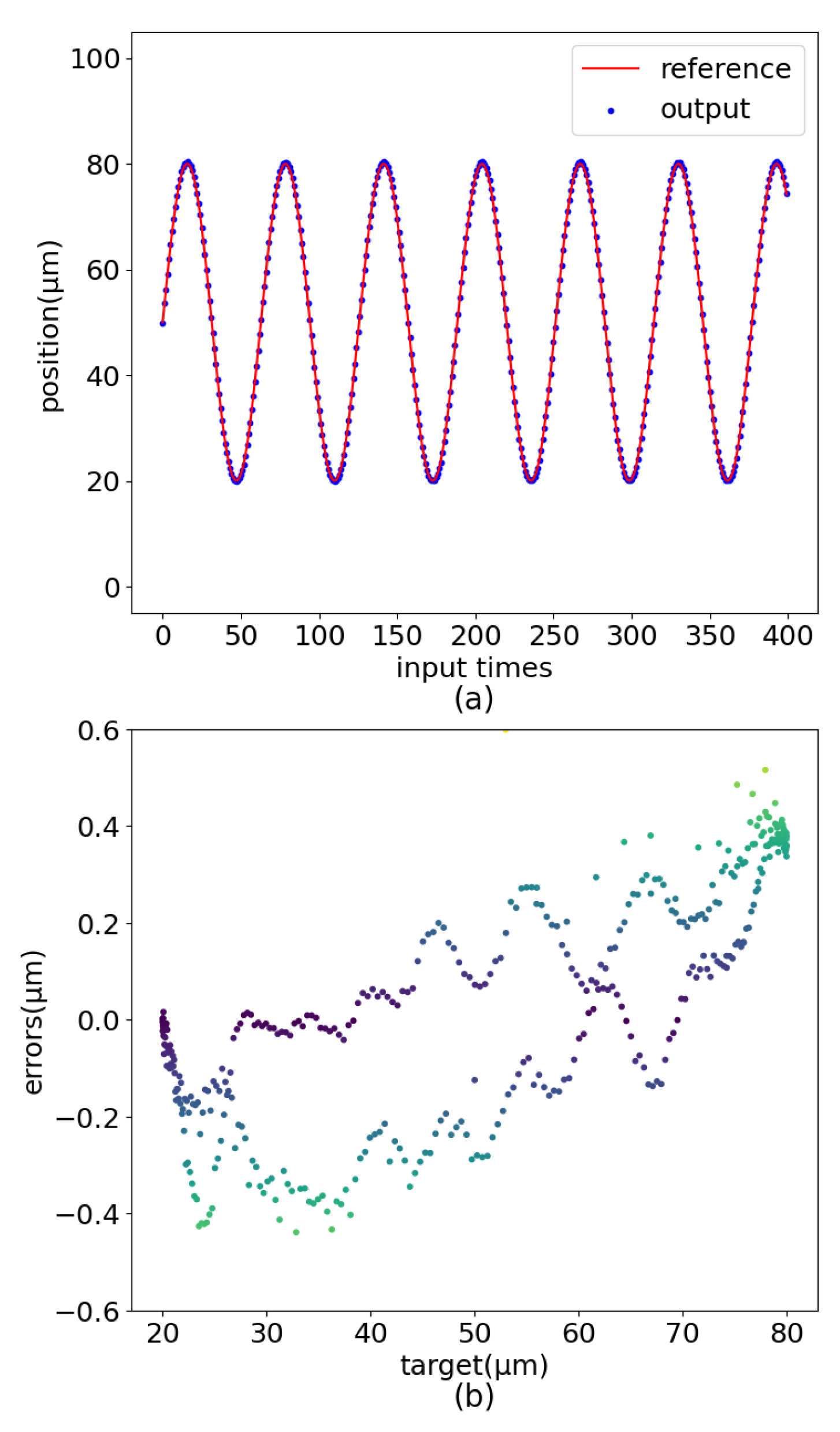
3.2.2. Experimental Test
3.3. Ablation Experiment
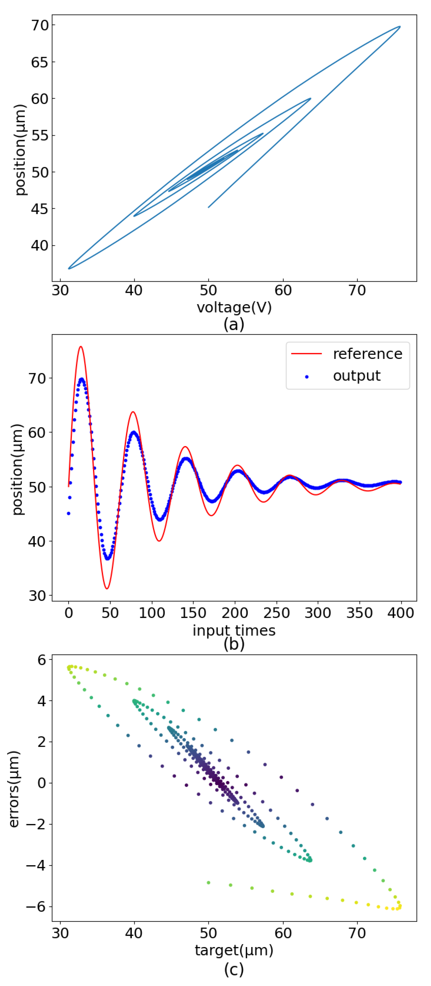
3.3.1. The Impact of MLP
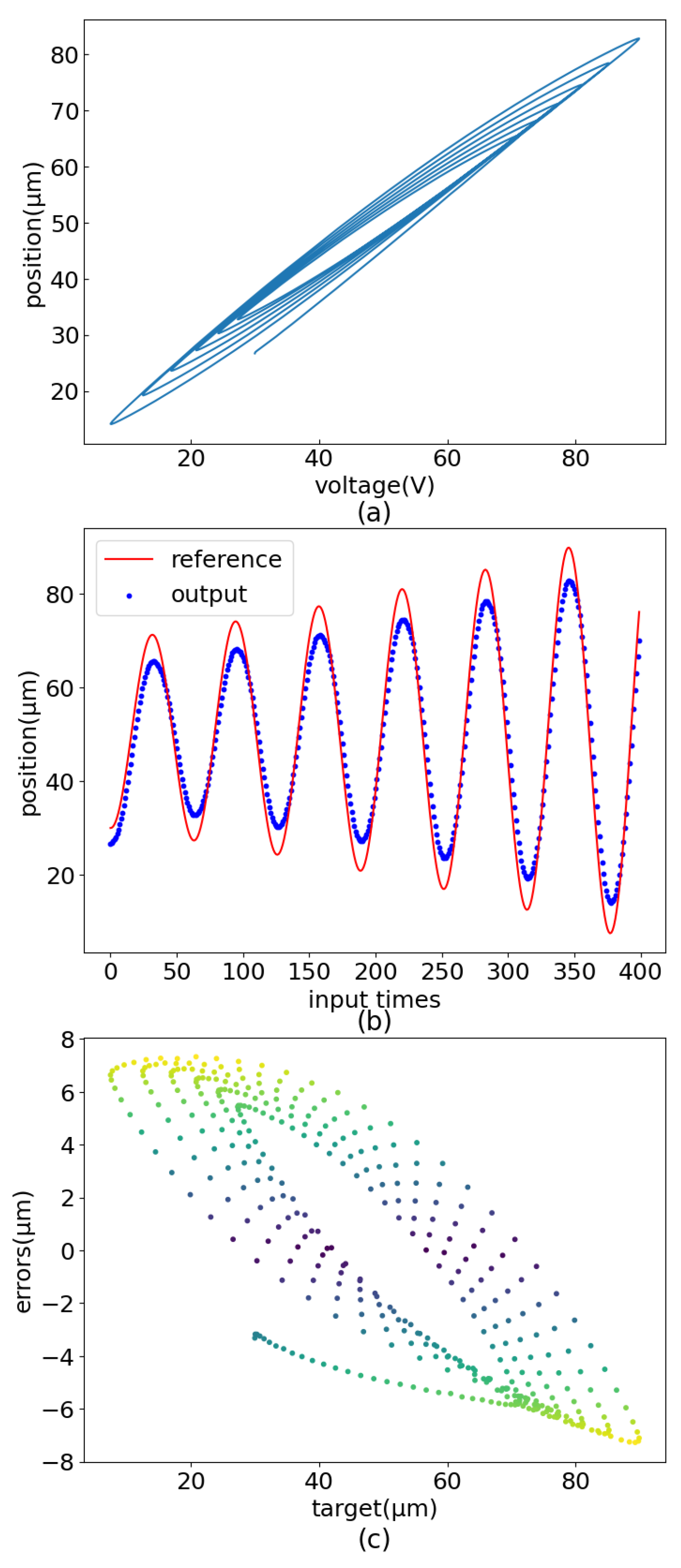
3.3.2. The Impact of Residual Connection
4. Conclusions
Author Contributions
Funding
Conflicts of Interest
Abbreviations
| MLP | Multilayer perceptron |
| PEA | Piezoelectric actuator |
| RBF | Radial basis function |
| GRU | Gated recurrent unit |
| SSRF | Shanghai Synchrotron Radiation Facility |
| PI | Physik Instrumente |
| MSE | Mean square error |
| ReLU | Linear rectification function |
References
- Shi, Y.; Gao, M.; Jia, W.; Yin, G.; Gao, X.; Du, Y.; Zheng, L. Intelligent commissioning system based on EPICS and differential evolution algorithm for synchrotron radiation beamline. Nucl. Tech. 2020, 43, 3–9. [Google Scholar]
- Jia, W.; Ma, S.; Zheng, L. The control system for water-cooled DCMS in SSRF. Nucl. Sci. Tech. 2015, 26, 26–31. [Google Scholar]
- Zhou, X. Research of Control in the Micro-Positioning System Actuated by Piezo-Ceramic. Ph.D. Thesis, Zhejiang University, Zhejiang, China, 2004. [Google Scholar]
- Gu, G.Y.; Zhu, L.M.; Su, C.Y.; Ding, H.; Fatikow, S. Modeling and control of piezo-actuated nanopositioning stages: A survey. IEEE Trans. Autom. Sci. Eng. 2014, 13, 313–332. [Google Scholar] [CrossRef]
- Landis, C.M. Non-linear constitutive modeling of ferroelectrics. Curr. Opin. Solid State Mater. Sci. 2004, 8, 59–69. [Google Scholar] [CrossRef]
- Gan, J.; Zhang, X. A review of nonlinear hysteresis modeling and control of piezoelectric actuators. AIP Adv. 2019, 9, 040702. [Google Scholar] [CrossRef] [Green Version]
- Preisach, F. Über die magnetische Nachwirkung. Z. für Phys. 1935, 94, 277–302. [Google Scholar] [CrossRef]
- Maas, J.; Schulte, T.; Frohleke, N. Model-based control for ultrasonic motors. IEEE/ASME Trans. Mechatron. 2000, 5, 165–180. [Google Scholar] [CrossRef] [Green Version]
- Lining, S.; Changhai, R.; Weibin, R.; Liguo, C.; Minxiu, K. Tracking control of piezoelectric actuator based on a new mathematical model. J. Micromechan. Microeng. 2004, 14, 1439. [Google Scholar] [CrossRef]
- Bouc, R. A mathematical model for hysteresis. Acta Acust. United Acust. 1971, 24, 16–25. [Google Scholar]
- Wen, Y.K. Method for random vibration of hysteretic systems. J. Eng. Mech. Div. 1976, 102, 249–263. [Google Scholar] [CrossRef]
- Delibas, B.; Arockiarajan, A.; Seemann, W. Rate dependent properties of perovskite type tetragonal piezoelectric materials using micromechanical model. Int. J. Solids Struct. 2006, 43, 697–712. [Google Scholar] [CrossRef] [Green Version]
- Kamlah, M.; Tsakmakis, C. Phenomenological modeling of the non-linear electro-mechanical coupling in ferroelectrics. Int. J. Solids Struct. 1999, 36, 669–695. [Google Scholar] [CrossRef]
- Liu, D.; Fang, Y.; Wang, H.; Dong, X. Adaptive novel MSGA-RBF neurocontrol for piezo-ceramic actuator suffering rate-dependent hysteresis. Sens. Actuators A Phys. 2019, 297, 111553. [Google Scholar] [CrossRef]
- Li, W.; Zhang, C.; Gao, W.; Zhou, M. Neural network self-tuning control for a piezoelectric actuator. Sensors 2020, 20, 3342. [Google Scholar] [CrossRef] [PubMed]
- Instrumente, P. E-709.CRG. Available online: https://www.physikinstrumente.store/eu/E-709.CRG/ (accessed on 14 July 2022).
- Instrumente, P. P-621.1CD. Available online: https://www.physikinstrumente.store/eu/p-621.1cd/ (accessed on 14 July 2022).
- Xiong, Y.; Jia, W.; Zhang, L.; Zheng, L. Research on Feedforward Compensation of Piezoelectric Ceramics Based on Deep Neural Network(DNN). Piezoelectrics Acoustooptics 2022, 44, 35. [Google Scholar]
- Zhang, A.; Li, M.; Lipton, Z.C.; Simola, A.J. Dive Into Deep Learning; Posts & Telecom Press Co., Ltd.: Beijing, China, 2019. [Google Scholar]
- Cho, K.; Van Merriënboer, B.; Gulcehre, C.; Bahdanau, D.; Bougares, F.; Schwenk, H.; Bengio, Y. Learning phrase representations using RNN encoder-decoder for statistical machine translation. arXiv 2014, arXiv:1406.1078. [Google Scholar]
- He, K.; Zhang, X.; Ren, S.; Sun, J. Deep residual learning for image recognition. In Proceedings of the IEEE Conference on Computer Vision and Pattern Recognition, Las Vegas, NV, USA, 27–30 June 2016; pp. 770–778. [Google Scholar]
- Kingma, D.P.; Ba, J. Adam: A method for stochastic optimization. arXiv 2014, arXiv:1412.6980. [Google Scholar]


| Layer Name | Input Dimension | Output Dimension | Bias | Hidden State Dimension |
|---|---|---|---|---|
| GRU layer | 3 | 3 | True | 128 |
| Linear 1 | 3 | 16 | True | / |
| Linear 2 | 16 | 32 | True | / |
| Linear 3 | 32 | 64 | True | / |
| Linear 4 | 64 | 128 | True | / |
| Linear 5 | 128 | 32 | True | / |
| Linear 6 | 32 | 4 | True | / |
| Linear 7 | 4 | 1 | True | / |
Publisher’s Note: MDPI stays neutral with regard to jurisdictional claims in published maps and institutional affiliations. |
© 2022 by the authors. Licensee MDPI, Basel, Switzerland. This article is an open access article distributed under the terms and conditions of the Creative Commons Attribution (CC BY) license (https://creativecommons.org/licenses/by/4.0/).
Share and Cite
Xiong, Y.; Jia, W.; Zhang, L.; Zhao, Y.; Zheng, L. Feedforward Control of Piezoelectric Ceramic Actuators Based on PEA-RNN. Sensors 2022, 22, 5387. https://doi.org/10.3390/s22145387
Xiong Y, Jia W, Zhang L, Zhao Y, Zheng L. Feedforward Control of Piezoelectric Ceramic Actuators Based on PEA-RNN. Sensors. 2022; 22(14):5387. https://doi.org/10.3390/s22145387
Chicago/Turabian StyleXiong, Yongcheng, Wenhong Jia, Limin Zhang, Ying Zhao, and Lifang Zheng. 2022. "Feedforward Control of Piezoelectric Ceramic Actuators Based on PEA-RNN" Sensors 22, no. 14: 5387. https://doi.org/10.3390/s22145387
APA StyleXiong, Y., Jia, W., Zhang, L., Zhao, Y., & Zheng, L. (2022). Feedforward Control of Piezoelectric Ceramic Actuators Based on PEA-RNN. Sensors, 22(14), 5387. https://doi.org/10.3390/s22145387