
The Impact of Data Augmentations on Deep Learning-Based Marine Object Classification in Benthic Image Transects


Abstract
:1. Introduction
2. Materials and Methods
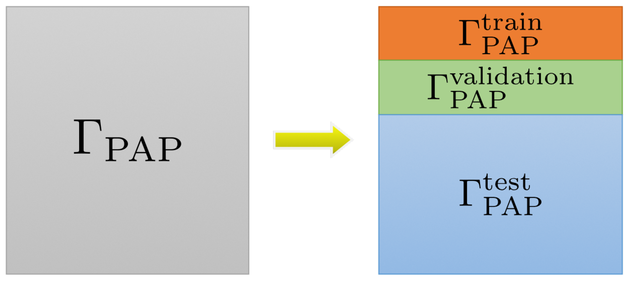
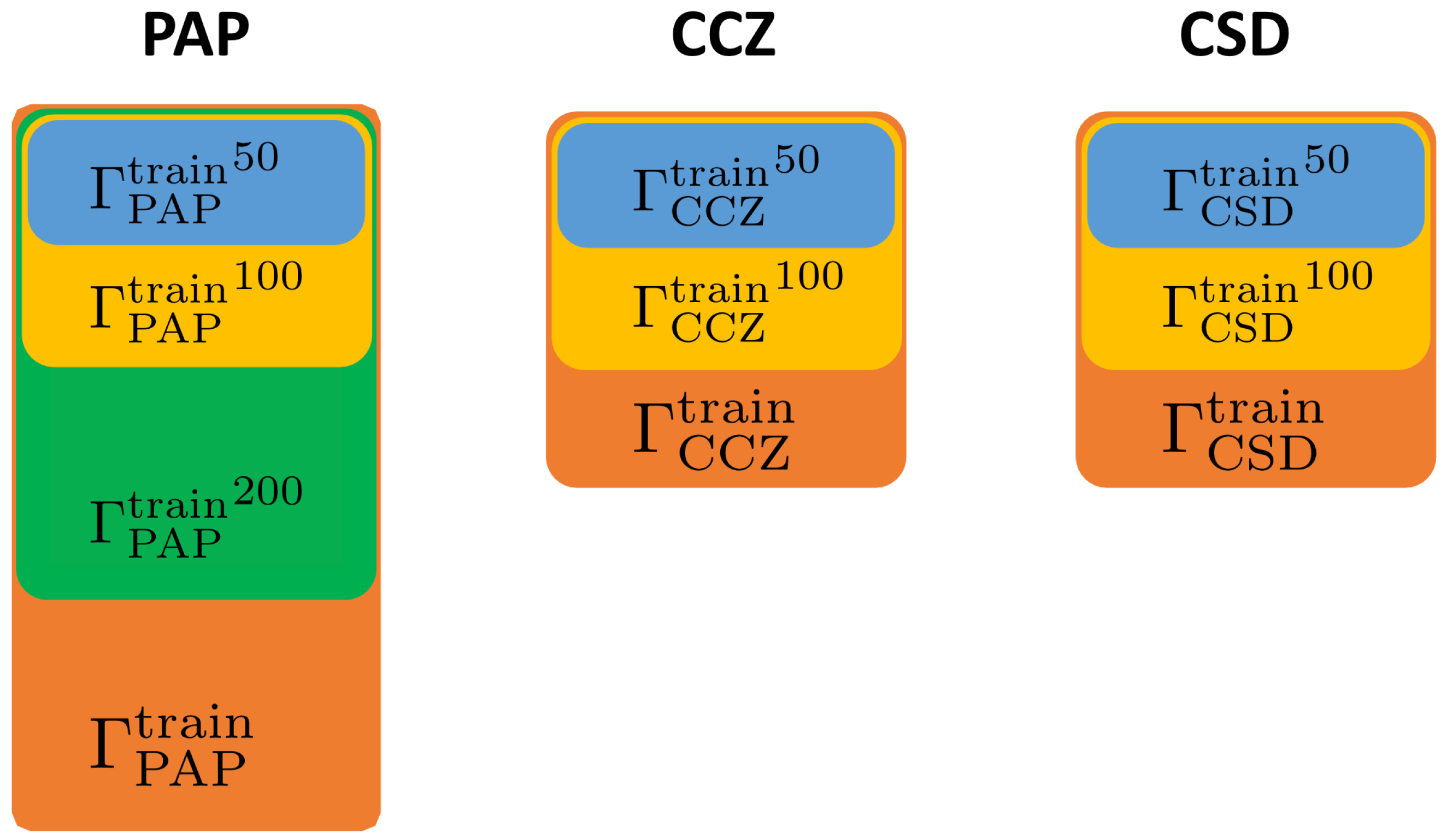
2.1. Data Sets
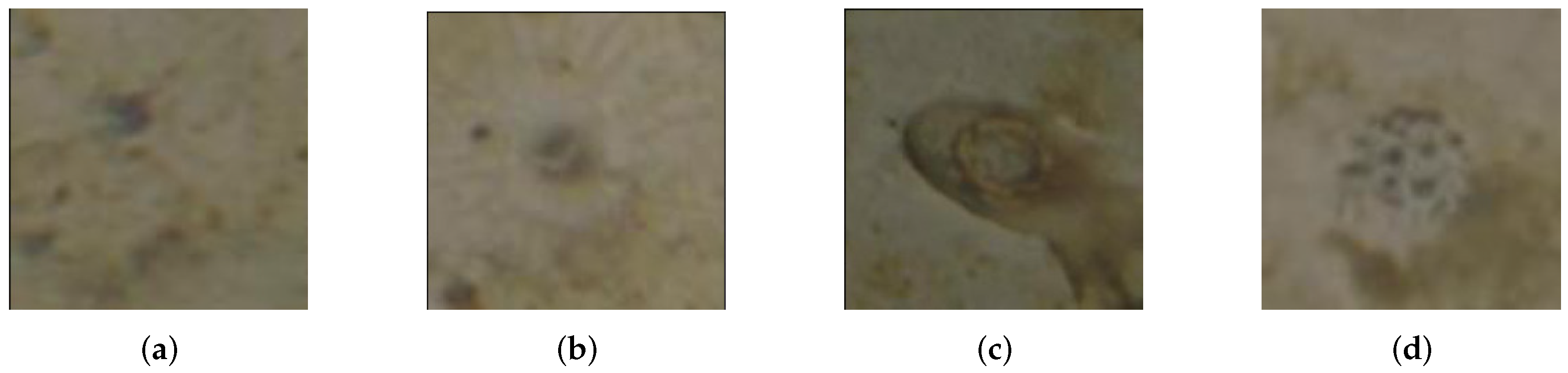
2.1.1. PAP
2.1.2. CCZ
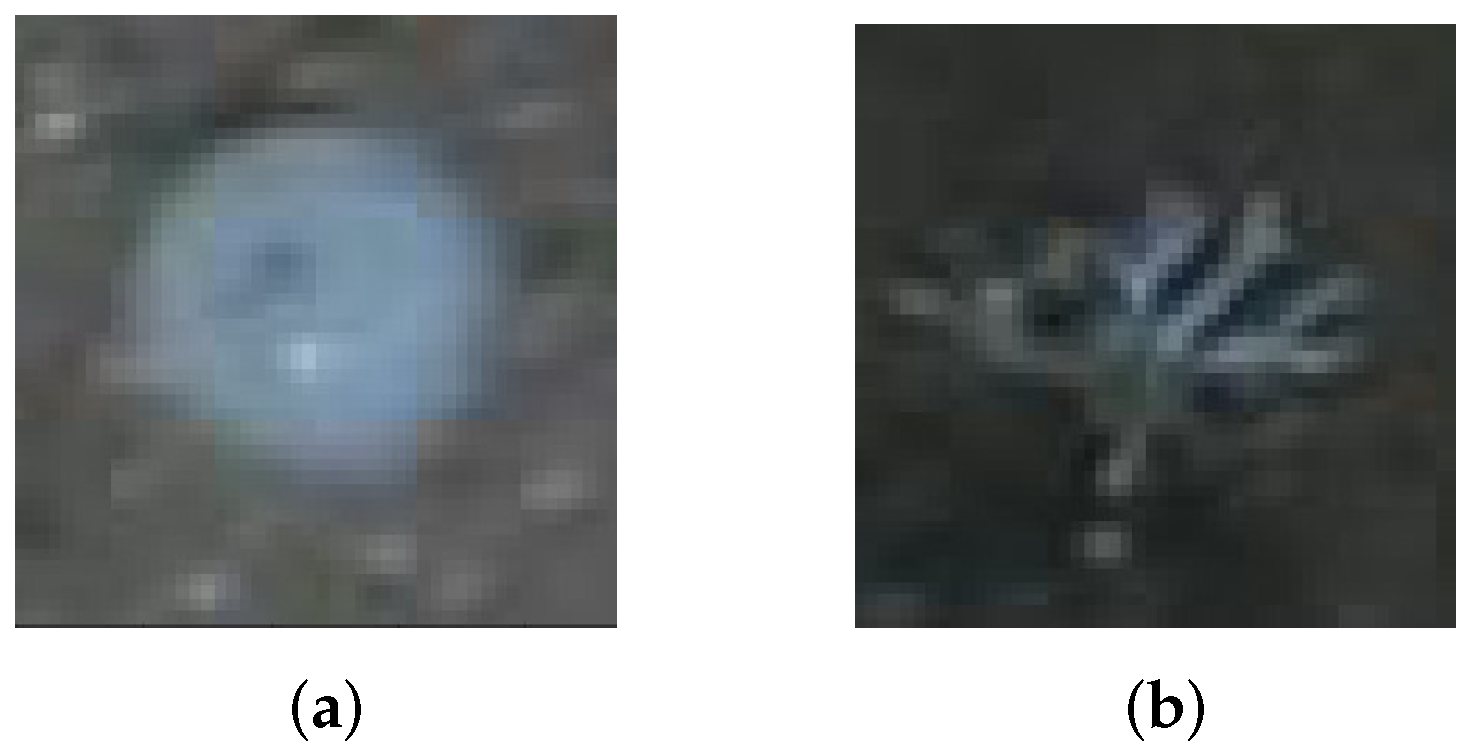
2.1.3. CSD
2.2. Model and Evaluation Criteria
2.3. Methods
3. Results
3.1. Experiment A: Performance of Data Augmentations on
3.2. Experiment B: Performance of Data Augmentations on
3.3. Experiment C: Performance of Data Augmentations on
3.4. Experiment D: Data Augmentation Policies
4. Discussion
5. Conclusions
Author Contributions
Funding
Data Availability Statement
Acknowledgments
Conflicts of Interest
Abbreviations
| AUV | Autonomous Underwater Vehicles |
| ROV | Remotely Operated Vehicles |
| SVM | Support Vector Machines |
| CNN | Convolutional Neural Networks |
| DA | Data Augmentation |
| GAN | Generative Adversarial Networks |
| PAP | Porcupine Abyssal Plane |
| CCZ | Clarion Clipperton Zone |
| CSD | Cityscapes Dataset |
Appendix A. Performance of DA Methods on and

| Random Rotation | Brightness | Contrast | Saturation | Random VerticalFlip | Random HorizontalFlip | ||||||
| 1° | 2.64% | 0.1 | 2.86% | 0.1 | 2.27% | 0.1 | 1.72% | 0.1 | 2.76% | 0.1 | 1.90% |
| 2° | 3.37% | 0.2 | 2.82% | 0.2 | 2.10% | 0.2 | 2.73% | 0.2 | 2.31% | 0.2 | 2.10% |
| 3° | 3.40% | 0.3 | 3.57% | 0.3 | 3.17% | 0.3 | 2.70% | 0.3 | 2.52% | 0.3 | 1.89% |
| 4° | 3.37% | 0.4 | 3.34% | 0.4 | 2.70% | 0.4 | 2.32% | 0.4 | 2.83% | 0.4 | 2.45% |
| 5° | 3.34% | 0.5 | 4.02% | 0.5 | 3.23% | 0.5 | 2.41% | 0.5 | 1.98% | 0.5 | 2.11% |
| 6° | 3.79% | 0.6 | 4.22% | 0.6 | 4.02% | 0.6 | 2.92% | 0.6 | 2.52% | 0.6 | 2.17% |
| 7° | 3.13% | 0.7 | 4.43% | 0.7 | 3.46% | 0.7 | 2.00% | 0.7 | 2.37% | 0.7 | 2.24% |
| 8° | 3.73% | 0.8 | 4.03% | 0.8 | 3.51% | 0.8 | 2.75% | 0.8 | 2.07% | 0.8 | 2.44% |
| 9° | 2.96% | 0.9 | 4.11% | 0.9 | 4.84% | 0.9 | 3.15% | 0.9 | 2.21% | 0.9 | 1.54% |
| 10° | 2.98% | 1 | 4.65% | 1 | 4.45% | 1 | 3.16% | 1 | 1.14% | 1 | 0.09% |
| 20° | 3.66% | 1.1 | 4.69% | 1.3 | 4.33% | 1.5 | 3.68% | Shear | |||
| 30° | 4.06% | 1.2 | 4.17% | 1.5 | 4.54% | 2 | 2.97% | ||||
| 40° | 4.71% | 1.3 | 4.41% | 1.8 | 4.48% | 3 | 3.48% | 5° | 2.01% | ||
| 50° | 4.94% | 1.4 | 4.91% | 2 | 4.65% | 4 | 3.62% | 10° | 3.30% | ||
| 60° | 5.21% | 1.5 | 4.91% | 2.5 | 4.37% | 5 | 3.58% | 20° | 3.45% | ||
| 70° | 4.83% | 1.6 | 4.74% | 3 | 4.50% | 6 | 4.03% | 30° | 4.14% | ||
| 80° | 4.49% | 1.7 | 5.08% | 3.5 | 4.11% | 7 | 4.05% | 40° | 3.26% | ||
| 90° | 5.07% | 1.8 | 4.79% | 4 | 4.50% | 8 | 4.17% | (0°, 0°, −5°, 5°) | 2.91% | ||
| 100° | 5.00% | 1.9 | 4.38% | 4.5 | 4.88% | 9 | 3.39% | (0°, 0°, −10°, 10°) | 3.31% | ||
| 110° | 5.37% | 2 | 5.08% | 5 | 5.40% | 10 | 3.94% | (0°, 0°, −20°, 20°) | 3.37% | ||
| 120° | 4.72% | Hue | Translate | (0°, 0°, −30°, 30°) | 3.20% | ||||||
| 130° | 4.92% | (0°, 0°, −40°, 40°) | 4.27% | ||||||||
| 140° | 4.80% | 0.1 | 3.00% | (0.1, 0.1) | 3.23% | (−5°, 5°, −5°, 5°) | 2.77% | ||||
| 150° | 4.76% | 0.2 | 3.38% | (0.2, 0.2) | 3.06% | (−10°, 10°, −10°, 10°) | 3.81% | ||||
| 160° | 5.61% | 0.3 | 2.98% | (0.3, 0.3) | 2.16% | (−20°, 20°, −20°, 20°) | 4.54% | ||||
| 170° | 5.43% | 0.4 | 2.63% | (0.4, 0.4) | 2.19% | (−30°, 30°, −30°, 30°) | 4.03% | ||||
| 180° | 5.17% | 0.5 | 3.12% | (0.5, 0.5) | −0.17% | (−40°, 40°, −40°, 40°) | 4.45% | ||||
| Random Rotation | Brightness | Contrast | Saturation | Random VerticalFlip | Random HorizontalFlip | ||||||
| 1° | 0.14% | 0.1 | 0.13% | 0.1 | 0.10% | 0.1 | 0.09% | 0.1 | −1.16% | 0.1 | 0.24% |
| 2° | 0.15% | 0.2 | 0.23% | 0.2 | 0.05% | 0.2 | 0.08% | 0.2 | −1.42% | 0.2 | 0.41% |
| 3° | 0.23% | 0.3 | 0.23% | 0.3 | 0.08% | 0.3 | 0.18% | 0.3 | −1.56% | 0.3 | 0.50% |
| 4° | 0.05% | 0.4 | 0.31% | 0.4 | 0.16% | 0.4 | 0.15% | 0.4 | −2.02% | 0.4 | 0.42% |
| 5° | 0.38% | 0.5 | 0.26% | 0.5 | 0.22% | 0.5 | 0.26% | 0.5 | −1.95% | 0.5 | 0.50% |
| 6° | 0.51% | 0.6 | 0.27% | 0.6 | 0.25% | 0.6 | 0.07% | 0.6 | −2.13% | 0.6 | 0.47% |
| 7° | 0.50% | 0.7 | −0.08% | 0.7 | −0.23% | 0.7 | 0.08% | 0.7 | −2.53% | 0.7 | 0.34% |
| 8° | 0.65% | 0.8 | 0.03% | 0.8 | −1.36% | 0.8 | 0.30% | 0.8 | −2.43% | 0.8 | 0.20% |
| 9° | 0.55% | 0.9 | 0.60% | 0.9 | 0.13% | 0.9 | 0.21% | 0.9 | −2.10% | 0.9 | 0.24% |
| 10° | −0.01% | 1 | 0.66% | 1 | 0.19% | 1 | 0.24% | 1 | −7.55% | 1 | 0.27% |
| 20° | −0.01% | 1.1 | 0.88% | 1.3 | 0.41% | 1.5 | 0.37% | Shear | |||
| 30° | −0.17% | 1.2 | 0.71% | 1.5 | 0.50% | 2 | 0.53% | ||||
| 40° | −0.20% | 1.3 | 0.45% | 1.8 | 0.45% | 3 | 0.63% | 5° | 0.36% | ||
| 50° | 0.10% | 1.4 | 0.29% | 2 | 0.62% | 4 | 1.02% | 10° | 0.44% | ||
| 60° | −0.45% | 1.5 | 0.75% | 2.5 | 0.70% | 5 | 1.27% | 20° | 0.11% | ||
| 70° | −0.56% | 1.6 | 0.70% | 3 | 0.52% | 6 | 1.14% | 30° | −0.03% | ||
| 80° | −3.18% | 1.7 | 0.95% | 3.5 | −0.31% | 7 | 1.24% | 40° | 0.01% | ||
| 90° | −2.44% | 1.8 | 0.57% | 4 | 0.31% | 8 | 1.30% | (0°, 0°, −5°, 5°) | 0.29% | ||
| 100° | −2.68% | 1.9 | 0.58% | 4.5 | 0.83% | 9 | 1.41% | (0°, 0°, −10°, 10°) | 0.33% | ||
| 110° | −2.11% | 2 | 0.32% | 5 | −0.36% | 10 | 1.35% | (0°, 0°, −20°, 20°) | 0.28% | ||
| 120° | −2.34% | Hue | Translate | (0°, 0°, −30°, 30°) | 0.48% | ||||||
| 130° | −1.83% | (0°, 0°, −40°, 40°) | 0.56% | ||||||||
| 140° | −3.11% | 0.1 | 0.50% | (0.1, 0.1) | −0.16% | (−5°, 5°, −5°, 5°) | 0.53% | ||||
| 150° | −3.36% | 0.2 | 0.57% | (0.2, 0.2) | −0.44% | (−10°, 10°, −10°, 10°) | 0.37% | ||||
| 160° | −3.38% | 0.3 | 0.69% | (0.3, 0.3) | −0.34% | (−20°, 20°, −20°, 20°) | 0.50% | ||||
| 170° | −3.22% | 0.4 | 0.52% | (0.4, 0.4) | −2.34% | (−30°, 30°, −30°, 30°) | 0.35% | ||||
| 180° | −3.12% | 0.5 | 0.52% | (0.5, 0.5) | −2.76% | (−40°, 40°, −40°, 40°) | −0.21% | ||||
Appendix B. Performance of DA Methods on and with Setting Seed to 3500
| Random Rotation | Brightness | Contrast | Saturation | Random VerticalFlip | Random HorizontalFlip | ||||||
| 1° | 3.26% | 0.1 | 1.76% | 0.1 | 1.06% | 0.1 | 0.75% | 0.1 | 2.26% | 0.1 | 1.60% |
| 2° | 4.34% | 0.2 | 2.57% | 0.2 | 1.52% | 0.2 | 0.88% | 0.2 | 2.64% | 0.2 | 1.75% |
| 3° | 4.96% | 0.3 | 3.19% | 0.3 | 2.12% | 0.3 | 1.32% | 0.3 | 2.87% | 0.3 | 2.00% |
| 4° | 5.21% | 0.4 | 3.16% | 0.4 | 1.24% | 0.4 | 1.63% | 0.4 | 2.91% | 0.4 | 2.08% |
| 5° | 5.45% | 0.5 | 3.59% | 0.5 | 2.98% | 0.5 | 1.63% | 0.5 | 2.99% | 0.5 | 1.97% |
| 6° | 5.58% | 0.6 | 3.94% | 0.6 | 3.29% | 0.6 | 1.94% | 0.6 | 2.79% | 0.6 | 1.93% |
| 7° | 5.65% | 0.7 | 4.16% | 0.7 | 3.61% | 0.7 | 2.16% | 0.7 | 2.72% | 0.7 | 1.88% |
| 8° | 5.68% | 0.8 | 4.70% | 0.8 | 4.01% | 0.8 | 2.11% | 0.8 | 2.74% | 0.8 | 1.67% |
| 9° | 5.75% | 0.9 | 5.30% | 0.9 | 4.43% | 0.9 | 2.51% | 0.9 | 2.55% | 0.9 | 1.21% |
| 10° | 5.58% | 1 | 5.76% | 1 | 4.84% | 1 | 2.48% | 1 | −0.51% | 1 | −0.36% |
| 20° | 5.61% | 1.1 | 5.34% | 1.3 | 4.83% | 1.5 | 2.69% | Shear | |||
| 30° | 5.81% | 1.2 | 5.34% | 1.5 | 4.83% | 2 | 3.00% | ||||
| 40° | 6.10% | 1.3 | 6.17% | 1.8 | 4.77% | 3 | 3.17% | 5° | 3.36% | ||
| 50° | 6.25% | 1.4 | 5.97% | 2 | 5.12% | 4 | 3.50% | 10° | 3.68% | ||
| 60° | 6.25% | 1.5 | 6.10% | 2.5 | 5.78% | 5 | 4.02% | 20° | 4.30% | ||
| 70° | 6.71% | 1.6 | 5.92% | 3 | 5.49% | 6 | 4.20% | 30° | 5.79% | ||
| 80° | 7.21% | 1.7 | 6.06% | 3.5 | 5.80% | 7 | 4.25% | 40° | 5.65% | ||
| 90° | 7.31% | 1.8 | 5.66% | 4 | 5.75% | 8 | 4.22% | (0°, 0°, −5°, 5°) | 4.17% | ||
| 100° | 7.59% | 1.9 | 6.13% | 4.5 | 5.12% | 9 | 4.48% | (0°, 0°, −10°, 10°) | 4.60% | ||
| 110° | 7.45% | 2 | 6.34% | 5 | 6.70% | 10 | 4.53% | (0°, 0°, −20°, 20°) | 4.98% | ||
| 120° | 7.21% | Hue | Translate | (0°, 0°, −30°, 30°) | 5.59% | ||||||
| 130° | 7.24% | (0°, 0°, −40°, 40°) | 5.98% | ||||||||
| 140° | 7.10% | 0.1 | 3.01% | (0.1, 0.1) | 5.50% | (−5°, 5°, −5°, 5°) | 5.32% | ||||
| 150° | 7.53% | 0.2 | 3.91% | (0.2, 0.2) | 4.20% | (−10°, 10°, −10°, 10°) | 5.07% | ||||
| 160° | 7.28% | 0.3 | 3.83% | (0.3, 0.3) | 3.31% | (−20°, 20°, −20°, 20°) | 5.52% | ||||
| 170° | 7.42% | 0.4 | 3.75% | (0.4, 0.4) | 1.54% | (−30°, 30°, −30°, 30°) | 6.32% | ||||
| 180° | 6.94% | 0.5 | 3.47% | (0.5, 0.5) | −3.24% | (−40°, 40°, −40°, 40°) | 5.41% | ||||
| Random Rotation | Brightness | Contrast | Saturation | Random VerticalFlip | Random HorizontalFlip | ||||||
| 1° | 4.14% | 0.1 | 2.76% | 0.1 | 2.45% | 0.1 | 1.51% | 0.1 | 3.61% | 0.1 | 2.72% |
| 2° | 4.11% | 0.2 | 3.18% | 0.2 | 3.23% | 0.2 | 1.62% | 0.2 | 3.20% | 0.2 | 3.02% |
| 3° | 4.60% | 0.3 | 4.03% | 0.3 | 3.23% | 0.3 | 1.21% | 0.3 | 3.23% | 0.3 | 3.10% |
| 4° | 4.56% | 0.4 | 4.08% | 0.4 | 3.93% | 0.4 | 2.08% | 0.4 | 3.10% | 0.4 | 3.28% |
| 5° | 4.53% | 0.5 | 4.49% | 0.5 | 4.25% | 0.5 | 2.10% | 0.5 | 3.14% | 0.5 | 3.04% |
| 6° | 4.51% | 0.6 | 4.75% | 0.6 | 4.42% | 0.6 | 2.12% | 0.6 | 3.11% | 0.6 | 3.12% |
| 7° | 4.43% | 0.7 | 4.35% | 0.7 | 4.59% | 0.7 | 2.34% | 0.7 | 2.90% | 0.7 | 3.23% |
| 8° | 4.69% | 0.8 | 4.47% | 0.8 | 4.66% | 0.8 | 2.00% | 0.8 | 2.57% | 0.8 | 3.10% |
| 9° | 4.97% | 0.9 | 4.86% | 0.9 | 4.79% | 0.9 | 2.11% | 0.9 | 2.32% | 0.9 | 2.81% |
| 10° | 4.61% | 1 | 4.58% | 1 | 3.44% | 1 | 2.22% | 1 | −1.51% | 1 | 0.16% |
| 20° | 5.28% | 1.1 | 4.45% | 1.3 | 5.09% | 1.5 | 2.73% | Shear | |||
| 30° | 5.16% | 1.2 | 4.83% | 1.5 | 4.50% | 2 | 2.71% | ||||
| 40° | 5.22% | 1.3 | 5.08% | 1.8 | 4.85% | 3 | 2.83% | 5° | 4.18% | ||
| 50° | 5.44% | 1.4 | 4.86% | 2 | 5.29% | 4 | 2.93% | 10° | 4.38% | ||
| 60° | 5.58% | 1.5 | 5.33% | 2.5 | 5.64% | 5 | 2.93% | 20° | 4.56% | ||
| 70° | 5.76% | 1.6 | 5.20% | 3 | 5.75% | 6 | 3.09% | 30° | 4.95% | ||
| 80° | 5.50% | 1.7 | 4.93% | 3.5 | 5.21% | 7 | 2.78% | 40° | 5.21% | ||
| 90° | 6.19% | 1.8 | 4.86% | 4 | 5.82% | 8 | 2.52% | (0°, 0°, −5°, 5°) | 4.13% | ||
| 100° | 6.31% | 1.9 | 4.89% | 4.5 | 5.38% | 9 | 2.60% | (0°, 0°, −10°, 10°) | 4.49% | ||
| 110° | 6.27% | 2 | 4.81% | 5 | 5.48% | 10 | 2.41% | (0°, 0°, −20°, 20°) | 4.22% | ||
| 120° | 5.73% | Hue | Translate | (0°, 0°, −30°, 30°) | 5.00% | ||||||
| 130° | 5.82% | (0°, 0°, −40°, 40°) | 4.77% | ||||||||
| 140° | 6.08% | 0.1 | 2.59% | (0.1, 0.1) | 4.30% | (−5°, 5°, −5°, 5°) | 4.98% | ||||
| 150° | 5.97% | 0.2 | 2.77% | (0.2, 0.2) | 4.07% | (−10°, 10°, −10°, 10°) | 4.97% | ||||
| 160° | 6.07% | 0.3 | 2.79% | (0.3, 0.3) | 3.54% | (−20°, 20°, −20°, 20°) | 5.29% | ||||
| 170° | 5.98% | 0.4 | 3.35% | (0.4, 0.4) | 1.94% | (−30°, 30°, −30°, 30°) | 4.84% | ||||
| 180° | 6.22% | 0.5 | 3.12% | (0.5, 0.5) | −1.62% | (−40°, 40°, −40°, 40°) | 4.72% | ||||
Appendix C. Impacts Comparison of Flip, Translate, and Hue


References
- Wynn, R.B.; Huvenne, V.A.; Le Bas, T.P.; Murton, B.J.; Connelly, D.P.; Bett, B.J.; Ruhl, H.A.; Morris, K.J.; Peakall, J.; Parsons, D.R.; et al. Autonomous Underwater Vehicles (AUVs): Their past, present and future contributions to the advancement of marine geoscience. Mar. Geol. 2014, 352, 451–468. [Google Scholar] [CrossRef] [Green Version]
- Christ, R.D.; Wernli, R.L., Sr. The ROV Manual: A User Guide for Remotely Operated Vehicles; Butterworth-Heinemann: Oxford, UK, 2013. [Google Scholar]
- Langenkämper, D.; Kevelaer, R.V.; Nattkemper, T.W. Strategies for tackling the class imbalance problem in marine image classification. In International Conference on Pattern Recognition; Springer: Berlin/Heidelberg, Germany, 2018; pp. 26–36. [Google Scholar]
- Wei, Y.; Yu, X.; Hu, Y.; Li, D. Development a zooplankton recognition method for dark field image. In Proceedings of the 2012 5th International Congress on Image and Signal Processing, Chongqing, China, 16–18 October 2012; pp. 861–865. [Google Scholar]
- Bewley, M.; Douillard, B.; Nourani-Vatani, N.; Friedman, A.; Pizarro, O.; Williams, S. Automated species detection: An experimental approach to kelp detection from sea-floor AUV images. In Proceedings of the Australasian Conference on Robotics and Automation, Wellingto, New Zealand, 3–5 December 2012. [Google Scholar]
- Lu, H.; Li, Y.; Uemura, T.; Ge, Z.; Xu, X.; He, L.; Serikawa, S.; Kim, H. FDCNet: Filtering deep convolutional network for marine organism classification. Multimed. Tools Appl. 2018, 77, 21847–21860. [Google Scholar] [CrossRef]
- Li, Y.; Lu, H.; Li, J.; Li, X.; Li, Y.; Serikawa, S. Underwater image de-scattering and classification by deep neural network. Comput. Electr. Eng. 2016, 54, 68–77. [Google Scholar] [CrossRef]
- Liu, X.; Jia, Z.; Hou, X.; Fu, M.; Ma, L.; Sun, Q. Real-time marine animal images classification by embedded system based on mobilenet and transfer learning. In Proceedings of the OCEANS 2019-Marseille, Marseille, France, 17–20 June 2019; pp. 1–5. [Google Scholar]
- Langenkämper, D.; Simon-Lledó, E.; Hosking, B.; Jones, D.O.; Nattkemper, T.W. On the impact of Citizen Science-derived data quality on deep learning based classification in marine images. PLoS ONE 2019, 14, e0218086. [Google Scholar] [CrossRef] [PubMed] [Green Version]
- Langenkämper, D.; Van Kevelaer, R.; Purser, A.; Nattkemper, T.W. Gear-induced concept drift in marine images and its effect on deep learning classification. Front. Mar. Sci. 2020, 7, 506. [Google Scholar] [CrossRef]
- Irfan, M.; Zheng, J.; Iqbal, M.; Arif, M.H. A novel feature extraction model to enhance underwater image classification. In International Symposium on Intelligent Computing Systems; Springer: Cham, Switzerland, 2020; pp. 78–91. [Google Scholar]
- Mahmood, A.; Bennamoun, M.; An, S.; Sohel, F.A.; Boussaid, F.; Hovey, R.; Kendrick, G.A.; Fisher, R.B. Deep image representations for coral image classification. IEEE J. Ocean. Eng. 2018, 44, 121–131. [Google Scholar] [CrossRef] [Green Version]
- Han, F.; Yao, J.; Zhu, H.; Wang, C. Marine organism detection and classification from underwater vision based on the deep CNN method. Math. Probl. Eng. 2020, 2020, 3937580. [Google Scholar] [CrossRef]
- Huang, H.; Zhou, H.; Yang, X.; Zhang, L.; Qi, L.; Zang, A.Y. Faster R-CNN for marine organisms detection and recognition using data augmentation. Neurocomputing 2019, 337, 372–384. [Google Scholar] [CrossRef]
- Xu, L.; Bennamoun, M.; An, S.; Sohel, F.; Boussaid, F. Deep learning for marine species recognition. In Handbook of Deep Learning Applications; Springer: Berlin/Heidelberg, Germany, 2019; pp. 129–145. [Google Scholar]
- Zhuang, P.; Xing, L.; Liu, Y.; Guo, S.; Qiao, Y. Marine Animal Detection and Recognition with Advanced Deep Learning Models. In CLEF (Working Notes); Springer: Berlin/Heidelberg, Germany, 2017. [Google Scholar]
- Xu, Y.; Zhang, Y.; Wang, H.; Liu, X. Underwater image classification using deep convolutional neural networks and data augmentation. In Proceedings of the 2017 IEEE International Conference on Signal Processing, Communications and Computing (ICSPCC), Xiamen, China, 22–25 October 2017; pp. 1–5. [Google Scholar]
- Wang, N.; Wang, Y.; Er, M.J. Review on deep learning techniques for marine object recognition: Architectures and algorithms. Control. Eng. Pract. 2020, 118, 104458. [Google Scholar] [CrossRef]
- NgoGia, T.; Li, Y.; Jin, D.; Guo, J.; Li, J.; Tang, Q. Real-Time Sea Cucumber Detection Based on YOLOv4-Tiny and Transfer Learning Using Data Augmentation. In International Conference on Swarm Intelligence; Springer: Cham, Switzerland, 2021; pp. 119–128. [Google Scholar]
- Xie, C.; Tan, M.; Gong, B.; Wang, J.; Yuille, A.L.; Le, Q.V. Adversarial examples improve image recognition. In Proceedings of the IEEE/CVF Conference on Computer Vision and Pattern Recognition, Virtual, 14–19 June 2020; pp. 819–828. [Google Scholar]
- Xiao, Q.; Liu, B.; Li, Z.; Ni, W.; Yang, Z.; Li, L. Progressive data augmentation method for remote sensing ship image classification based on imaging simulation system and neural style transfer. IEEE J. Sel. Top. Appl. Earth Obs. Remote Sens. 2021, 14, 9176–9186. [Google Scholar] [CrossRef]
- Chu, P.; Bian, X.; Liu, S.; Ling, H. Feature space augmentation for long-tailed data. In European Conference on Computer Vision; Springer: Berlin/Heidelberg, Germany, 2020; pp. 694–710. [Google Scholar]
- DeVries, T.; Taylor, G.W. Dataset augmentation in feature space. arXiv 2017, arXiv:1702.05538. [Google Scholar]
- Li, C.; Huang, Z.; Xu, J.; Yan, Y. Data Augmentation using Conditional Generative Adversarial Network for Underwater Target Recognition. In Proceedings of the 2019 IEEE International Conference on Signal, Information and Data Processing (ICSIDP), Chongqing, China, 11–13 December 2019; pp. 1–5. [Google Scholar]
- Antoniou, A.; Storkey, A.; Edwards, H. Augmenting image classifiers using data augmentation generative adversarial networks. In International Conference on Artificial Neural Networks; Springer: Berlin/Heidelberg, Germany, 2018; pp. 594–603. [Google Scholar]
- Cubuk, E.D.; Zoph, B.; Mane, D.; Vasudevan, V.; Le, Q.V. Autoaugment: Learning augmentation strategies from data. In Proceedings of the IEEE/CVF Conference on Computer Vision and Pattern Recognition, Long Beach, CA, USA, 16–20 June 2019; pp. 113–123. [Google Scholar]
- Lemley, J.; Bazrafkan, S.; Corcoran, P. Smart augmentation learning an optimal data augmentation strategy. IEEE Access 2017, 5, 5858–5869. [Google Scholar] [CrossRef]
- Dabouei, A.; Soleymani, S.; Taherkhani, F.; Nasrabadi, N.M. Supermix: Supervising the mixing data augmentation. In Proceedings of the IEEE/CVF Conference on Computer Vision and Pattern Recognition, Virtual, 19–25 June 2021; pp. 13794–13803. [Google Scholar]
- Naveed, H. Survey: Image mixing and deleting for data augmentation. arXiv 2021, arXiv:2106.07085. [Google Scholar]
- Kang, G.; Dong, X.; Zheng, L.; Yang, Y. Patchshuffle regularization. arXiv 2017, arXiv:1707.07103. [Google Scholar]
- O’Gara, S.; McGuinness, K. Comparing Data Augmentation Strategies for Deep Image Classification; Technological University Dublin: Dublin, Ireland, 2019. [Google Scholar]
- Engstrom, L.; Tran, B.; Tsipras, D.; Schmidt, L.; Madry, A. A Rotation and a Translation Suffice: Fooling Cnns with Simple Transformations. arXiv 2018, arXiv:171202779. [Google Scholar]
- Shorten, C.; Khoshgoftaar, T.M. A survey on image data augmentation for deep learning. J. Big Data 2019, 6, 60. [Google Scholar] [CrossRef]
- Lim, S.; Kim, I.; Kim, T.; Kim, C.; Kim, S. Fast autoaugment. Adv. Neural Inf. Process. Syst. 2019, 32, 6665–6675. [Google Scholar]
- Shijie, J.; Ping, W.; Peiyi, J.; Siping, H. Research on data augmentation for image classification based on convolution neural networks. In Proceedings of the 2017 Chinese Automation Congress (CAC), Jinan, China, 20–22 October 2017; pp. 4165–4170. [Google Scholar]
- Durden, J.M.; Bett, B.J.; Ruhl, H.A. Subtle variation in abyssal terrain induces significant change in benthic megafaunal abundance, diversity, and community structure. Prog. Oceanogr. 2020, 186, 102395. [Google Scholar] [CrossRef]
- Hartman, S.E.; Bett, B.J.; Durden, J.M.; Henson, S.A.; Iversen, M.; Jeffreys, R.M.; Horton, T.; Lampitt, R.; Gates, A.R. Enduring science: Three decades of observing the Northeast Atlantic from the Porcupine Abyssal Plain Sustained Observatory (PAP-SO). Prog. Oceanogr. 2021, 191, 102508. [Google Scholar] [CrossRef]
- Morris, K.J.; Bett, B.J.; Durden, J.M.; Huvenne, V.A.; Milligan, R.; Jones, D.O.; McPhail, S.; Robert, K.; Bailey, D.M.; Ruhl, H.A. A new method for ecological surveying of the abyss using autonomous underwater vehicle photography. Limnol. Oceanogr. Methods 2014, 12, 795–809. [Google Scholar] [CrossRef] [Green Version]
- Simon-Lledó, E.; Bett, B.J.; Huvenne, V.A.; Schoening, T.; Benoist, N.M.; Jeffreys, R.M.; Durden, J.M.; Jones, D.O. Megafaunal variation in the abyssal landscape of the Clarion Clipperton Zone. Prog. Oceanogr. 2019, 170, 119–133. [Google Scholar] [CrossRef] [PubMed]
- Cordts, M.; Omran, M.; Ramos, S.; Rehfeld, T.; Enzweiler, M.; Benenson, R.; Franke, U.; Roth, S.; Schiele, B. The Cityscapes Dataset for Semantic Urban Scene Understanding. In Proceedings of the IEEE Conference on Computer Vision and Pattern Recognition Recognition (CVPR), Las Vegas, NV, USA, 27–30 June 2016. pp. 3213–3223.
- Krizhevsky, A.; Sutskever, I.; Hinton, G.E. Imagenet classification with deep convolutional neural networks. Adv. Neural Inf. Process. Syst. 2012, 25, 1097–1105. [Google Scholar] [CrossRef]


| Ophiuroidea | Cnidaria | Amperima | Foraminifera | |
|---|---|---|---|---|
| 50 | 50 | 50 | 50 | |
| 100 | 100 | 100 | 100 | |
| 200 | 200 | 200 | 200 | |
| 300 | 300 | 300 | 300 | |
| 200 | 200 | 200 | 200 | |
| 8883 | 8861 | 5202 | 2132 |
| Sponge | Coral | |
|---|---|---|
| 50 | 50 | |
| 100 | 100 | |
| 150 | 150 | |
| 150 | 150 | |
| 1236 | 700 |
| Car | Bicycle | |
|---|---|---|
| 50 | 50 | |
| 100 | 100 | |
| 150 | 150 | |
| 200 | 200 | |
| 24,371 | 3208 |
| Random Rotation | Brightness | Contrast | Saturation | Random VerticalFlip | Random HorizontalFlip | ||||||
| 1° | 3.82% | 0.1 | 2.79% | 0.1 | 1.97% | 0.1 | 0.92% | 0.1 | 2.68% | 0.1 | 1.65% |
| 2° | 5.11% | 0.2 | 3.95% | 0.2 | 2.85% | 0.2 | 1.35% | 0.2 | 3.15% | 0.2 | 1.93% |
| 3° | 5.69% | 0.3 | 4.38% | 0.3 | 3.34% | 0.3 | 1.96% | 0.3 | 3.24% | 0.3 | 1.95% |
| 4° | 5.89% | 0.4 | 4.40% | 0.4 | 3.71% | 0.4 | 2.18% | 0.4 | 3.51% | 0.4 | 1.99% |
| 5° | 6.11% | 0.5 | 4.90% | 0.5 | 4.15% | 0.5 | 2.46% | 0.5 | 3.57% | 0.5 | 2.11% |
| 6° | 6.01% | 0.6 | 5.35% | 0.6 | 4.53% | 0.6 | 2.81% | 0.6 | 3.66% | 0.6 | 2.14% |
| 7° | 6.03% | 0.7 | 5.61% | 0.7 | 4.66% | 0.7 | 3.11% | 0.7 | 3.57% | 0.7 | 2.11% |
| 8° | 6.30% | 0.8 | 5.64% | 0.8 | 5.19% | 0.8 | 3.06% | 0.8 | 3.31% | 0.8 | 1.80% |
| 9° | 6.10% | 0.9 | 6.24% | 0.9 | 5.59% | 0.9 | 2.97% | 0.9 | 3.12% | 0.9 | 1.56% |
| 10° | 6.01% | 1 | 6.82% | 1 | 6.22% | 1 | 2.95% | 1 | 0.34% | 1 | –1.16% |
| 20° | 6.85% | 1.1 | 6.25% | 1.3 | 6.33% | 1.5 | 3.27% | Shear | |||
| 30° | 6.97% | 1.2 | 6.87% | 1.5 | 5.87% | 2 | 3.29% | ||||
| 40° | 6.71% | 1.3 | 6.75% | 1.8 | 6.18% | 3 | 4.08% | 5° | 4.05% | ||
| 50° | 6.96% | 1.4 | 7.01% | 2 | 6.29% | 4 | 4.67% | 10° | 3.92% | ||
| 60° | 7.41% | 1.5 | 7.22% | 2.5 | 5.86% | 5 | 4.97% | 20° | 4.34% | ||
| 70° | 7.17% | 1.6 | 6.56% | 3 | 7.13% | 6 | 5.43% | 30° | 4.93% | ||
| 80° | 7.39% | 1.7 | 6.95% | 3.5 | 7.00% | 7 | 5.49% | 40° | 5.48% | ||
| 90° | 7.61% | 1.8 | 7.01% | 4 | 6.88% | 8 | 5.72% | (0°, 0°, −5°, 5°) | 4.20% | ||
| 100° | 8.02% | 1.9 | 7.11% | 4.5 | 6.59% | 9 | 5.83% | (0°, 0°, −10°, 10°) | 5.38% | ||
| 110° | 7.84% | 2 | 7.74% | 5 | 7.70% | 10 | 5.99% | (0°, 0°, −20°, 20°) | 6.20% | ||
| 120° | 7.70% | Hue | Translate | (0°,0°, −30°, 30°) | 6.06% | ||||||
| 130° | 7.69% | (0°, 0°, −40°, 40°) | 6.47% | ||||||||
| 140° | 7.76% | 0.1 | 4.17% | (0.1, 0.1) | 5.59% | (−5°, 5°, −5°, 5°) | 5.89% | ||||
| 150° | 7.31% | 0.2 | 5.13% | (0.2, 0.2) | 4.72% | (−10°, 10°, −10°, 10°) | 5.75% | ||||
| 160° | 7.47% | 0.3 | 4.86% | (0.3, 0.3) | 4.21% | (−20°, 20°, −20°, 20°) | 6.22% | ||||
| 170° | 7.11% | 0.4 | 4.52% | (0.4, 0.4) | 2.53% | (−30°, 30°, −30°, 30°) | 6.68% | ||||
| 180° | 7.55% | 0.5 | 4.70% | (0.5, 0.5) | 1.40% | (−40°, 40°, −40°, 40°) | 6.58% | ||||
| Random Rotation | Brightness | Contrast | Saturation | Random VerticalFlip | Random HorizontalFlip | ||||||
| 1° | 1.30% | 0.1 | 1.19% | 0.1 | 0.69% | 0.1 | 0.25% | 0.1 | 0.94% | 0.1 | 0.77% |
| 2° | 1.55% | 0.2 | 1.22% | 0.2 | 1.41% | 0.2 | 0.34% | 0.2 | 0.81% | 0.2 | 0.92% |
| 3° | 2.18% | 0.3 | 1.38% | 0.3 | 1.41% | 0.3 | 0.42% | 0.3 | 1.01% | 0.3 | 0.80% |
| 4° | 2.11% | 0.4 | 1.70% | 0.4 | 1.48% | 0.4 | 0.57% | 0.4 | 0.86% | 0.4 | 0.88% |
| 5° | 2.01% | 0.5 | 1.75% | 0.5 | 1.56% | 0.5 | 0.74% | 0.5 | 1.31% | 0.5 | 0.79% |
| 6° | 1.94% | 0.6 | 1.85% | 0.6 | 1.76% | 0.6 | 1.11% | 0.6 | 0.89% | 0.6 | 0.82% |
| 7° | 2.08% | 0.7 | 2.13% | 0.7 | 1.95% | 0.7 | 1.24% | 0.7 | 0.77% | 0.7 | 0.74% |
| 8° | 1.55% | 0.8 | 2.15% | 0.8 | 2.12% | 0.8 | 0.38% | 0.8 | 0.56% | 0.8 | 0.70% |
| 9° | 2.18% | 0.9 | 2.59% | 0.9 | 1.82% | 0.9 | 1.09% | 0.9 | 0.78% | 0.9 | 0.62% |
| 10° | 2.15% | 1 | 2.57% | 1 | 2.05% | 1 | 1.27% | 1 | −0.43% | 1 | −0.43% |
| 20° | 2.14% | 1.1 | 2.34% | 1.3 | 1.84% | 1.5 | 0.81% | Shear | |||
| 30° | 2.53% | 1.2 | 2.43% | 1.5 | 2.15% | 2 | 1.49% | ||||
| 40° | 2.17% | 1.3 | 2.34% | 1.8 | 2.32% | 3 | 1.75% | 5° | 1.70% | ||
| 50° | 2.62% | 1.4 | 2.35% | 2 | 1.81% | 4 | 1.72% | 10° | 1.85% | ||
| 60° | 2.74% | 1.5 | 2.06% | 2.5 | 1.94% | 5 | 1.80% | 20° | 1.78% | ||
| 70° | 2.86% | 1.6 | 2.43% | 3 | 2.15% | 6 | 1.85% | 30° | 1.53% | ||
| 80° | 2.45% | 1.7 | 2.35% | 3.5 | 2.26% | 7 | 1.86% | 40° | 2.13% | ||
| 90° | 3.06% | 1.8 | 2.47% | 4 | 2.19% | 8 | 1.61% | (0°, 0°, −5°, 5°) | 1.63% | ||
| 100° | 3.17% | 1.9 | 2.52% | 4.5 | 2.40% | 9 | 1.76% | (0°, 0°, −10°, 10°) | 2.34% | ||
| 110° | 3.09% | 2 | 2.39% | 5 | 2.28% | 10 | 1.72% | (0°, 0°, −20°, 20°) | 1.72% | ||
| 120° | 3.25% | Hue | Translate | (0°, 0°, −30°, 30°) | 2.06% | ||||||
| 130° | 2.96% | (0°, 0°, −40°, 40°) | 2.33% | ||||||||
| 140° | 3.14% | 0.1 | 1.45% | (0.1, 0.1) | 2.00% | (−5°, 5°, −5°, 5°) | 2.20% | ||||
| 150° | 3.27% | 0.2 | 1.61% | (0.2, 0.2) | 1.67% | (−10°, 10°, −10°, 10°) | 2.22% | ||||
| 160° | 3.08% | 0.3 | 1.94% | (0.3, 0.3) | 1.57% | (−20°, 20°, −20°, 20°) | 2.40% | ||||
| 170° | 3.29% | 0.4 | 1.73% | (0.4, 0.4) | 0.69% | (−30°, 30°, −30°, 30°) | 2.29% | ||||
| 180° | 3.23% | 0.5 | 1.72% | (0.5, 0.5) | 0.21% | (−40°, 40°, −40°, 40°) | 2.40% | ||||
| Random Rotation | Brightness | Contrast | Saturation | Random VerticalFlip | Random HorizontalFlip | ||||||
| 1° | 3.07% | 0.1 | 1.86% | 0.1 | 2.12% | 0.1 | 0.77% | 0.1 | 2.93% | 0.1 | 2.27% |
| 2° | 4.13% | 0.2 | 2.77% | 0.2 | 2.40% | 0.2 | 1.20% | 0.2 | 3.05% | 0.2 | 2.67% |
| 3° | 3.99% | 0.3 | 3.18% | 0.3 | 3.08% | 0.3 | 1.26% | 0.3 | 3.24% | 0.3 | 2.60% |
| 4° | 4.39% | 0.4 | 4.03% | 0.4 | 4.01% | 0.4 | 1.66% | 0.4 | 3.01% | 0.4 | 2.53% |
| 5° | 4.91% | 0.5 | 4.26% | 0.5 | 4.32% | 0.5 | 1.82% | 0.5 | 2.80% | 0.5 | 2.60% |
| 6° | 4.98% | 0.6 | 4.50% | 0.6 | 4.88% | 0.6 | 1.37% | 0.6 | 3.04% | 0.6 | 2.85% |
| 7° | 5.00% | 0.7 | 4.94% | 0.7 | 4.91% | 0.7 | 1.76% | 0.7 | 3.01% | 0.7 | 2.78% |
| 8° | 5.12% | 0.8 | 4.51% | 0.8 | 5.36% | 0.8 | 2.07% | 0.8 | 3.15% | 0.8 | 2.65% |
| 9° | 4.97% | 0.9 | 4.44% | 0.9 | 4.77% | 0.9 | 2.08% | 0.9 | 2.63% | 0.9 | 2.31% |
| 10° | 5.31% | 1 | 5.32% | 1 | 4.97% | 1 | 2.29% | 1 | −0.93% | 1 | −0.99% |
| 20° | 5.70% | 1.1 | 5.35% | 1.3 | 4.86% | 1.5 | 2.21% | Shear | |||
| 30° | 5.54% | 1.2 | 5.19% | 1.5 | 5.06% | 2 | 1.27% | ||||
| 40° | 6.35% | 1.3 | 5.10% | 1.8 | 5.03% | 3 | 1.67% | 5° | 2.70% | ||
| 50° | 6.11% | 1.4 | 5.43% | 2 | 5.15% | 4 | 1.42% | 10° | 3.39% | ||
| 60° | 5.81% | 1.5 | 5.16% | 2.5 | 5.39% | 5 | 2.09% | 20° | 4.95% | ||
| 70° | 6.17% | 1.6 | 4.71% | 3 | 4.95% | 6 | 2.20% | 30° | 5.55% | ||
| 80° | 6.48% | 1.7 | 5.53% | 3.5 | 4.56% | 7 | 2.03% | 40° | 5.44% | ||
| 90° | 6.69% | 1.8 | 5.09% | 4 | 4.88% | 8 | 2.43% | (0°, 0°, −5°, 5°) | 4.71% | ||
| 100° | 6.31% | 1.9 | 5.54% | 4.5 | 5.30% | 9 | 2.19% | (0°, 0°, −10°, 10°) | 5.16% | ||
| 110° | 6.57% | 2 | 5.28% | 5 | 5.16% | 10 | 1.85% | (0°, 0°, −20°, 20°) | 4.95% | ||
| 120° | 6.85% | Hue | Translate | (0°, 0°, −30°, 30°) | 5.23% | ||||||
| 130° | 6.66% | (0°, 0°, −40°, 40°) | 5.51% | ||||||||
| 140° | 6.31% | 0.1 | 3.18% | (0.1, 0.1) | 4.98% | (−5°, 5°, −5°, 5°) | 5.55% | ||||
| 150° | 7.14% | 0.2 | 3.96% | (0.2, 0.2) | 4.19% | (−10°, 10°, −10°, 10°) | 5.60% | ||||
| 160° | 6.95% | 0.3 | 3.98% | (0.3, 0.3) | 3.76% | (−20°, 20°, −20°, 20°) | 5.64% | ||||
| 170° | 6.80% | 0.4 | 3.48% | (0.4, 0.4) | 3.09% | (−30°, 30°, −30°, 30°) | 5.91% | ||||
| 180° | 6.73% | 0.5 | 2.95% | (0.5, 0.5) | −0.15% | (−40°, 40°, −40°, 40°) | 6.11% | ||||
| Random Rotation | Brightness | Contrast | Saturation | Random VerticalFlip | Random HorizontalFlip | ||||||
| 1° | 1.84% | 0.1 | 0.73% | 0.1 | 0.53% | 0.1 | 0.32% | 0.1 | 1.50% | 0.1 | 0.92% |
| 2° | 2.01% | 0.2 | 1.40% | 0.2 | 0.91% | 0.2 | 0.40% | 0.2 | 1.29% | 0.2 | 0.92% |
| 3° | 1.81% | 0.3 | 1.59% | 0.3 | 1.18% | 0.3 | 0.60% | 0.3 | 1.26% | 0.3 | 0.99% |
| 4° | 2.02% | 0.4 | 1.74% | 0.4 | 1.76% | 0.4 | 1.06% | 0.4 | 1.25% | 0.4 | 1.26% |
| 5° | 2.18% | 0.5 | 1.73% | 0.5 | 1.72% | 0.5 | 1.32% | 0.5 | 1.10% | 0.5 | 1.14% |
| 6° | 1.82% | 0.6 | 1.65% | 0.6 | 1.87% | 0.6 | 1.29% | 0.6 | 1.17% | 0.6 | 1.24% |
| 7° | 1.80% | 0.7 | 2.47% | 0.7 | 2.34% | 0.7 | 1.48% | 0.7 | 0.95% | 0.7 | 1.20% |
| 8° | 2.12% | 0.8 | 1.93% | 0.8 | 2.52% | 0.8 | 1.56% | 0.8 | 0.84% | 0.8 | 0.90% |
| 9° | 2.26% | 0.9 | 2.13% | 0.9 | 2.55% | 0.9 | 1.91% | 0.9 | 0.73% | 0.9 | 0.87% |
| 10° | 2.39% | 1 | 2.57% | 1 | 3.08% | 1 | 2.05% | 1 | −1.07% | 1 | −0.19% |
| 20° | 2.71% | 1.1 | 2.22% | 1.3 | 3.33% | 1.5 | 2.46% | Shear | |||
| 30° | 3.19% | 1.2 | 2.83% | 1.5 | 3.22% | 2 | 2.46% | ||||
| 40° | 2.45% | 1.3 | 2.41% | 1.8 | 3.32% | 3 | 2.40% | 5° | 1.36% | ||
| 50° | 2.60% | 1.4 | 2.49% | 2 | 3.00% | 4 | 2.35% | 10° | 1.59% | ||
| 60° | 2.18% | 1.5 | 2.66% | 2.5 | 3.10% | 5 | 2.13% | 20° | 1.96% | ||
| 70° | 3.09% | 1.6 | 2.87% | 3 | 3.03% | 6 | 1.88% | 30° | 2.37% | ||
| 80° | 3.16% | 1.7 | 2.90% | 3.5 | 3.13% | 7 | 1.53% | 40° | 2.99% | ||
| 90° | 3.76% | 1.8 | 2.43% | 4 | 3.10% | 8 | 1.73% | (0°, 0°, −5°, 5°) | 1.88% | ||
| 100° | 3.57% | 1.9 | 2.54% | 4.5 | 3.19% | 9 | 2.00% | (0°, 0°, −10°, 10°) | 1.66% | ||
| 110° | 3.68% | 2 | 3.14% | 5 | 3.33% | 10 | 2.18% | (0°, 0°, −20°, 20°) | 1.85% | ||
| 120° | 3.66% | Hue | Translate | (0°, 0°, −30°, 30°) | 2.32% | ||||||
| 130° | 3.56% | (0°, 0°, −40°, 40°) | 2.75% | ||||||||
| 140° | 3.32% | 0.1 | 1.40% | (0.1, 0.1) | 1.63% | (−5°, 5°, −5°, 5°) | 2.02% | ||||
| 150° | 3.17% | 0.2 | 1.68% | (0.2, 0.2) | 1.44% | (−10°, 10°, −10°, 10°) | 2.14% | ||||
| 160° | 3.74% | 0.3 | 1.69% | (0.3, 0.3) | 1.02% | (−20°, 20°, −20°, 20°) | 2.30% | ||||
| 170° | 3.93% | 0.4 | 1.57% | (0.4, 0.4) | −0.66% | (−30°, 30°, −30°, 30°) | 2.16% | ||||
| 180° | 3.64% | 0.5 | 1.62% | (0.5, 0.5) | −0.90% | (−40°, 40°, −40°, 40°) | 2.11% | ||||
| Random Rotation | Brightness | Contrast | Saturation | Random VerticalFlip | Random HorizontalFlip | ||||||
| 1° | −0.08% | 0.1 | −0.12% | 0.1 | −0.09% | 0.1 | 0.07% | 0.1 | −1.95% | 0.1 | 0.59% |
| 2° | 0.32% | 0.2 | 0.06% | 0.2 | −0.14% | 0.2 | 0.17% | 0.2 | −1.43% | 0.2 | 0.46% |
| 3° | 0.63% | 0.3 | 0.12% | 0.3 | −0.06% | 0.3 | 0.42% | 0.3 | −1.52% | 0.3 | 0.63% |
| 4° | 0.39% | 0.4 | −0.16% | 0.4 | −0.08% | 0.4 | 0.63% | 0.4 | −1.39% | 0.4 | 0.68% |
| 5° | 0.30% | 0.5 | −0.04% | 0.5 | −0.16% | 0.5 | 0.62% | 0.5 | −1.69% | 0.5 | 0.59% |
| 6° | 0.52% | 0.6 | 0.27% | 0.6 | −0.06% | 0.6 | 0.69% | 0.6 | −1.82% | 0.6 | 0.57% |
| 7° | 0.42% | 0.7 | 0.20% | 0.7 | 0.18% | 0.7 | 0.61% | 0.7 | −2.07% | 0.7 | 0.56% |
| 8° | 0.34% | 0.8 | 0.17% | 0.8 | −0.35% | 0.8 | 0.77% | 0.8 | −2.49% | 0.8 | 0.51% |
| 9° | 0.31% | 0.9 | −0.18% | 0.9 | −0.08% | 0.9 | 0.75% | 0.9 | −2.80% | 0.9 | 0.37% |
| 10° | 0.19% | 1 | −0.19% | 1 | −0.56% | 1 | 0.90% | 1 | −8.53% | 1 | −0.30% |
| 20° | −0.67% | 1.1 | −0.60% | 1.3 | −0.67% | 1.5 | 1.18% | Shear | |||
| 30° | −0.98% | 1.2 | −0.67% | 1.5 | −0.25% | 2 | 1.33% | ||||
| 40° | −1.61% | 1.3 | −0.33% | 1.8 | 0.02% | 3 | 1.36% | 5° | −0.14% | ||
| 50° | −0.47% | 1.4 | 0.19% | 2 | −0.25% | 4 | 1.30% | 10° | 0.25% | ||
| 60° | −0.88% | 1.5 | 0.07% | 2.5 | −0.33% | 5 | 1.22% | 20° | −0.06% | ||
| 70° | −1.87% | 1.6 | −0.40% | 3 | −0.08% | 6 | 1.16% | 30° | −0.42% | ||
| 80° | −2.67% | 1.7 | 0.03% | 3.5 | 0.22% | 7 | 1.26% | 40° | −0.25% | ||
| 90° | −2.35% | 1.8 | 0.11% | 4 | 0.04% | 8 | 1.30% | (0°, 0°, −5°, 5°) | 0.92% | ||
| 100° | −2.79% | 1.9 | 0.57% | 4.5 | 0.59% | 9 | 1.15% | (0°, 0°, −10°, 10°) | 0.89% | ||
| 110° | −2.57% | 2 | 0.40% | 5 | 1.13% | 10 | 1.25% | (0°, 0°, −20°, 20°) | 0.31% | ||
| 120° | −2.94% | Hue | Translate | (0°, 0°, −30°, 30°) | 0.19% | ||||||
| 130° | −3.85% | (0°, 0°, −40°, 40°) | −0.10% | ||||||||
| 140° | −3.81% | 0.1 | 0.53% | (0.1, 0.1) | −0.38% | (−5°, 5°, −5°, 5°) | 0.37% | ||||
| 150° | −3.89% | 0.2 | 0.27% | (0.2, 0.2) | −0.14% | (−10°, 10°, −10°, 10°) | 0.55% | ||||
| 160° | −4.80% | 0.3 | 0.16% | (0.3, 0.3) | −0.57% | (−20°, 20°, −20°, 20°) | 0.14% | ||||
| 170° | −4.31% | 0.4 | −0.01% | (0.4, 0.4) | −2.02% | (−30°, 30°, −30°, 30°) | −0.37% | ||||
| 180° | −4.28% | 0.5 | 0.10% | (0.5, 0.5) | −2.46% | (−40°, 40°, −40°, 40°) | −1.18% | ||||
| Random Rotation | Brightness | Contrast | Saturation | Random VerticalFlip | Random HorizontalFlip | ||||||
| 1° | 0.35% | 0.1 | 0.23% | 0.1 | 0.25% | 0.1 | 0.13% | 0.1 | −1.22% | 0.1 | 0.26% |
| 2° | 0.55% | 0.2 | 0.40% | 0.2 | 0.46% | 0.2 | 0.24% | 0.2 | −1.37% | 0.2 | 0.53% |
| 3° | 0.74% | 0.3 | 0.34% | 0.3 | 0.55% | 0.3 | 0.23% | 0.3 | −1.78% | 0.3 | 0.50% |
| 4° | 0.09% | 0.4 | 0.62% | 0.4 | 0.53% | 0.4 | 0.29% | 0.4 | −1.82% | 0.4 | 0.44% |
| 5° | 0.55% | 0.5 | 0.73% | 0.5 | 0.62% | 0.5 | 0.21% | 0.5 | −2.21% | 0.5 | 0.37% |
| 6° | 0.75% | 0.6 | 0.91% | 0.6 | 0.37% | 0.6 | 0.29% | 0.6 | −2.31% | 0.6 | 0.65% |
| 7° | 0.83% | 0.7 | 0.51% | 0.7 | 0.90% | 0.7 | 0.42% | 0.7 | −2.33% | 0.7 | 0.47% |
| 8° | 0.55% | 0.8 | 0.86% | 0.8 | 0.59% | 0.8 | 0.49% | 0.8 | −2.33% | 0.8 | 0.32% |
| 9° | 0.84% | 0.9 | 0.86% | 0.9 | 0.18% | 0.9 | 0.48% | 0.9 | −1.64% | 0.9 | 0.57% |
| 10° | −0.21% | 1 | 0.81% | 1 | 1.07% | 1 | 0.49% | 1 | −8.28% | 1 | 0.48% |
| 20° | 0.32% | 1.1 | 0.91% | 1.3 | 0.35% | 1.5 | 0.70% | Shear | |||
| 30° | 0.31% | 1.2 | 1.18% | 1.5 | 1.37% | 2 | 0.81% | ||||
| 40° | −0.16% | 1.3 | 1.33% | 1.8 | 0.87% | 3 | 0.82% | 5° | 0.28% | ||
| 50° | −0.18% | 1.4 | 1.11% | 2 | 1.00% | 4 | 0.94% | 10° | 0.78% | ||
| 60° | −0.14% | 1.5 | 1.24% | 2.5 | 0.83% | 5 | 1.02% | 20° | 0.50% | ||
| 70° | −0.08% | 1.6 | 1.33% | 3 | 0.93% | 6 | 1.09% | 30° | 0.17% | ||
| 80° | −0.64% | 1.7 | 0.56% | 3.5 | 0.75% | 7 | 1.27% | 40° | −0.11% | ||
| 90° | −2.72% | 1.8 | 0.96% | 4 | 1.40% | 8 | 1.31% | (0°, 0°, −5°, 5°) | 0.56% | ||
| 100° | −2.48% | 1.9 | 0.96% | 4.5 | 0.73% | 9 | 1.31% | (0°, 0°, −10°, 10°) | −0.18% | ||
| 110° | −3.08% | 2 | 1.26% | 5 | 1.08% | 10 | 1.11% | (0°, 0°, −20°, 20°) | 0.32% | ||
| 120° | −2.34% | Hue | Translate | (0°, 0°, −30°, 30°) | 0.31% | ||||||
| 130° | −2.49% | (0°, 0°, −40°, 40°) | −0.27% | ||||||||
| 140° | −3.21% | 0.1 | 0.60% | (0.1, 0.1) | 0.13% | (−5°, 5°, −5°, 5°) | 0.87% | ||||
| 150° | −3.02% | 0.2 | 0.54% | (0.2, 0.2) | −1.52% | (−10°, 10°, −10°, 10°) | 0.91% | ||||
| 160° | −2.56% | 0.3 | 0.56% | (0.3, 0.3) | −0.62% | (−20°, 20°, −20°, 20°) | −0.72% | ||||
| 170° | −3.26% | 0.4 | 0.61% | (0.4, 0.4) | −1.47% | (−30°, 30°, −30°, 30°) | −0.14% | ||||
| 180° | −4.57% | 0.5 | 0.48% | (0.5, 0.5) | −0.79% | (−40°, 40°, −40°, 40°) | −0.06% | ||||
| DA Policy | Function of Each Policy |
|---|---|
| RBC_1 | |
| RBC_2 | |
| RBC_3 | |
| RBC_4 | |
| RBC_5 | |
| RBCS | ) |
| AA_IP | AA_CP | RBC_1 | RBC_2 | RBC_3 | RBC_4 | RBC_5 | RBCS | |
|---|---|---|---|---|---|---|---|---|
| +9.59% | +9.43% | +10.63% | +10.45% | +10.49% | +10.38% | +10.86% | +10.57% | |
| +5.48% | +5.07% | +6.32% | +6.35% | +6.26% | +6.07% | +5.86% | +6.14% | |
| +3.19% | +2.89% | +3.73% | +3.66% | +3.72% | +3.80% | +3.61% | +3.66% | |
| +2.48% | +2.66% | +2.76% | +2.84% | +2.80% | +2.91% | +2.83% | +2.88% | |
| +6.23% | +5.06% | +6.78% | +6.77% | +6.73% | +7.31% | +7.05% | +7.10% | |
| +4.26% | +3.81% | +4.52% | +4.08% | +4.68% | +4.21% | +4.74% | +4.58% | |
| +2.41% | +2.04% | +2.39% | +2.52% | +2.50% | +2.37% | +2.58% | +2.46% | |
| +0.94% | +0.92% | −1.47% | −1.73% | −1.54% | −0.81% | −0.82% | −2.67% | |
| +2.57% | +1.06% | −2.61% | −1.95% | −1.99% | −2.12% | −1.80% | −1.53% | |
| +1.17% | +1.44% | −1.02% | −1.76% | −1.31% | −2.12% | −1.08% | −1.65% |
Publisher’s Note: MDPI stays neutral with regard to jurisdictional claims in published maps and institutional affiliations. |
© 2022 by the authors. Licensee MDPI, Basel, Switzerland. This article is an open access article distributed under the terms and conditions of the Creative Commons Attribution (CC BY) license (https://creativecommons.org/licenses/by/4.0/).
Share and Cite
Tan, M.; Langenkämper, D.; Nattkemper, T.W. The Impact of Data Augmentations on Deep Learning-Based Marine Object Classification in Benthic Image Transects. Sensors 2022, 22, 5383. https://doi.org/10.3390/s22145383
Tan M, Langenkämper D, Nattkemper TW. The Impact of Data Augmentations on Deep Learning-Based Marine Object Classification in Benthic Image Transects. Sensors. 2022; 22(14):5383. https://doi.org/10.3390/s22145383
Chicago/Turabian StyleTan, Mingkun, Daniel Langenkämper, and Tim W. Nattkemper. 2022. "The Impact of Data Augmentations on Deep Learning-Based Marine Object Classification in Benthic Image Transects" Sensors 22, no. 14: 5383. https://doi.org/10.3390/s22145383
APA StyleTan, M., Langenkämper, D., & Nattkemper, T. W. (2022). The Impact of Data Augmentations on Deep Learning-Based Marine Object Classification in Benthic Image Transects. Sensors, 22(14), 5383. https://doi.org/10.3390/s22145383