
Color Occlusion Face Recognition Method Based on Quaternion Non-Convex Sparse Constraint Mechanism


Abstract
:1. Introduction
2. Main Research Work
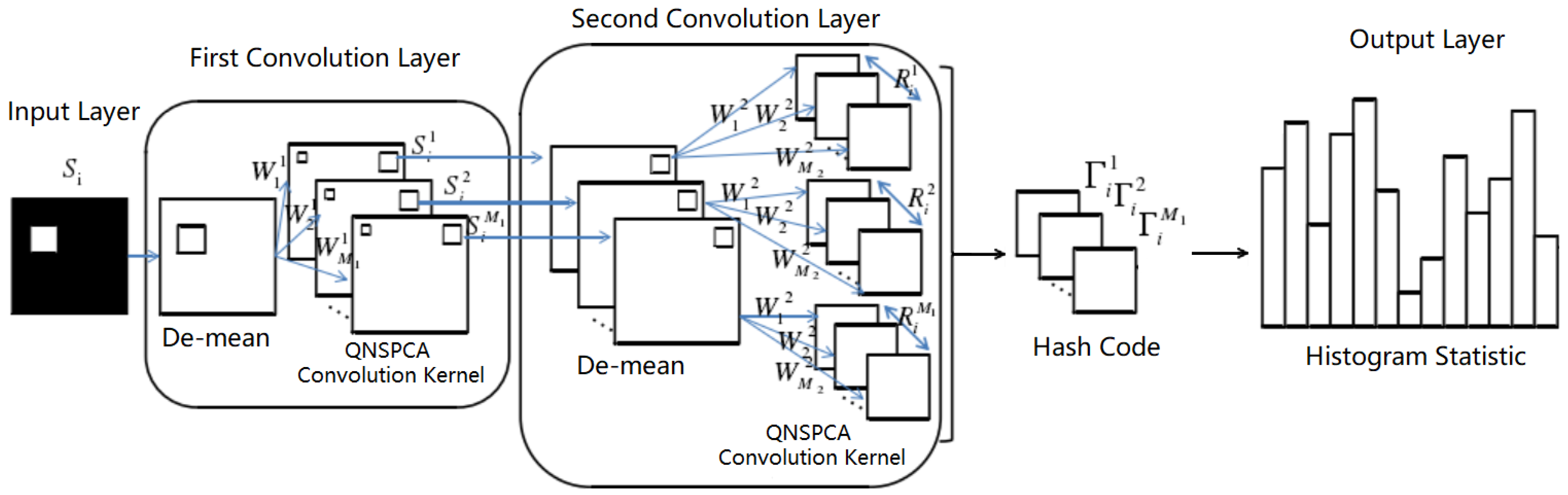
2.1. The Establishment of QNSPCANet Model
2.1.1. Quaternion Representation of Color Images
2.1.2. Quaternion Non-Convex Sparse Principal Component Analysis Convolution Kernel
2.1.3. Two-Order Convolution Layer
2.1.4. Pooling and Feature Output
- (1)
- QNSPCANet uses regularization to compute sparse convolution kernels, which has higher sparse efficiency and can reduce computational complexity compared with general regularization;
- (2)
- Sparse regularization is beneficial to identify important variables related to outliers, while the principal component convolution check outliers calculated by non-convex regularization of strong sparsity have better robustness and improve model recognition performance;
- (3)
- For the image with occlusion, the sparse principal component convolution kernel can reduce the influence of outliers in the occlusion area and further improve the recognition accuracy.
2.2. Lp Non-Convex Sparse Optimization Method for Model Parameters
2.2.1. Coordinate Descent
2.2.2. Fixed Point Iterative Method
3. Algorithm Simulation Experiments
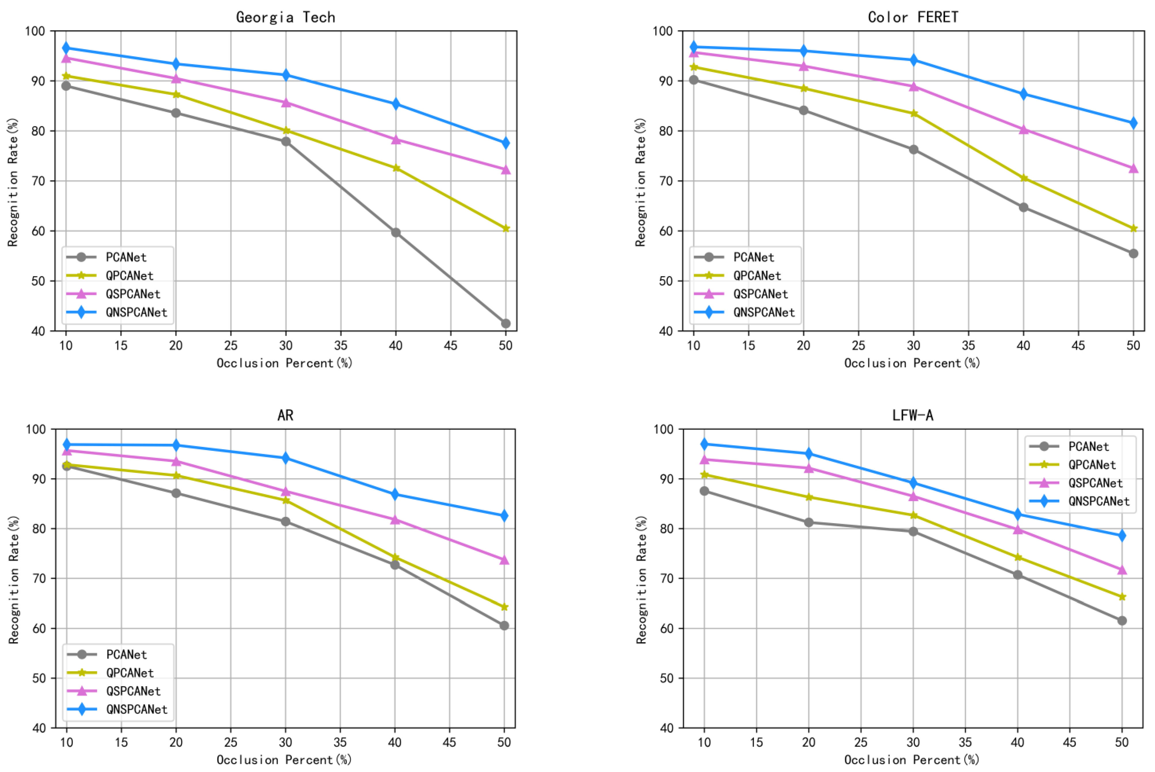
3.1. Comparison of Algorithm Performance under Different Occlusion Conditions
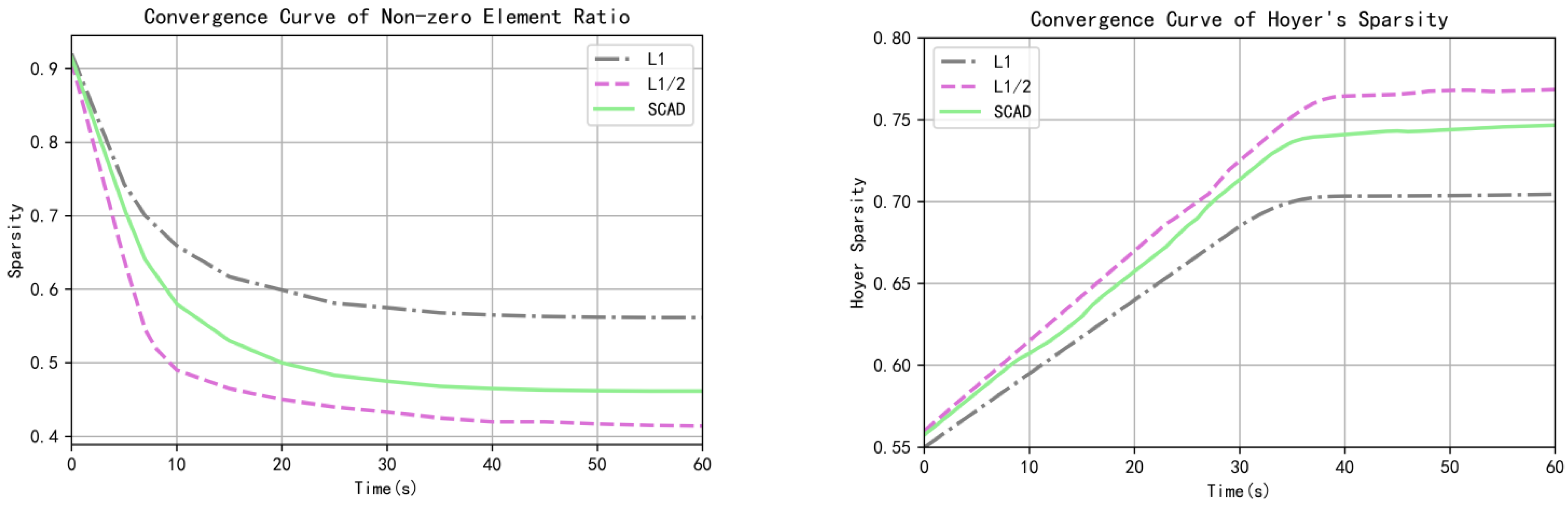
3.2. Algorithm Sparsity Verification
3.3. Algorithm Robustness Verification
4. Conclusions
Author Contributions
Funding
Institutional Review Board Statement
Informed Consent Statement
Conflicts of Interest
References
- Li, Z. Face recognition technology research status review. Electron. Technol. Softw. Eng. 2020, 13, 106–107. [Google Scholar]
- Zhao, K.; Jin, X.; Wang, Y. A review of research on small sample learning. J. Softw. 2021, 32, 349–369. [Google Scholar]
- Chan, T.-H.; Jia, K.; Gao, S.; Lu, J.; Zeng, Z.; Ma, Y. PCANet: A Simple Deep Learning Baseline for Image Classification? IEEE Trans. Image Process. 2015, 24, 5017–5032. [Google Scholar] [CrossRef] [PubMed] [Green Version]
- Bao, S.; Song, X.; Hu, G.; Yang, X.; Wang, C. Colour face recognition using fuzzy quaternion-based discriminant analysis. Int. J. Mach. Learn. Cybern. 2019, 10, 385–395. [Google Scholar] [CrossRef]
- Turk, M.; Pentland, A. Eigenfaces for recognition. J. Cogn. Neurosci. 1991, 3, 71–86. [Google Scholar] [CrossRef] [PubMed]
- Torres, L.; Reutter, J.; Lorente, L. The importance of the color information in face recognition. In Proceedings of the 6th IEEE International Conference on Image Processing, Kobe, Japan, 24–28 October 1999; pp. 627–631. [Google Scholar]
- Yang, J.; Liu, C. Color Image Discriminant Models and Algorithms for Face Recognition. IEEE Trans. Neural Netw. 2008, 19, 2088–2098. [Google Scholar] [CrossRef] [PubMed]
- Li, Y.; Zhu, S.; Zhu, L. Face recognition algorithm based on quaternion principal component analysis. Signal Processing 2007, 2, 214–216. [Google Scholar]
- Xiao, X.; Zhou, Y. Two-Dimensional Quaternion PCA and Sparse PCA. IEEE Trans. Neural Netw. Learn. Syst. 2019, 30, 2028–2042. [Google Scholar] [CrossRef] [PubMed]
- Xu, Z.; Zhang, H.; Wang, Y.; Change, X.; Liang, Y. L_(1/2) regularization. Sci. China Inf. Sci. 2010, 53, 1159–1169. [Google Scholar] [CrossRef] [Green Version]
- Yang, X. Two-stage method for sparse principal component analysis. Prog. Appl. Math. 2017, 6, 1174–1181. [Google Scholar]
- Scarselli, F.; Gori, M.; Tsoi, A.C.; Hagenbuchner, M.; Monfardini, G. The Graph Neural Network Model. IEEE Trans. Neural Netw. A Publ. IEEE Neural Netw. Counc. 2008, 20, 61–80. [Google Scholar] [CrossRef] [PubMed] [Green Version]
- Huang, X.; Ren, M.; Hu, Z. An Improvement of K-Medoids Clustering Algorithm Based on Fixed Point Iteration. Int. J. Data Warehous. Min. 2020, 16, 84–94. [Google Scholar] [CrossRef]
- Georgia Tech Face Database. Available online: http://www.anefian.com/research/face_reco.html (accessed on 20 May 2022).
- Color FERET Database. Available online: https://www.nist.gov/itl/products-and-services/color-feret-database (accessed on 20 May 2022).
- Martinez, A.; Benavente, R. The AR Face Database; Technical Report; The Computer Vision Center (CVC): Barcelona, Spain, 1998. [Google Scholar]
- Gary, B.; Manu, R.; Tamara, B.; Erik, L. Labeled Faces in the Wild: A Database for Studying Face Recognition in Unconstrained Environments; University of Massachusetts: Amherst, MA, USA, 2007; pp. 7–49. [Google Scholar]
- Asem, M. A 3D-based Pose Invariant Face Recognition at a Distance Framework. IEEE Trans. Inf. Forensics Secur. 2014, 9, 2158–2169. [Google Scholar]
- Cao, L.; Li, H.; Guo, H.; Wang, B. Robust PCA for Face Recognition with Occlusion Using Symmetry Information. In Proceedings of the 2019 IEEE 16th International Conference on Networking, Sensing and Control (ICNSC), Banff, AB, Canada, 9–11 May 2019; pp. 323–328. [Google Scholar] [CrossRef]
- Cen, F.; Wang, G. Dictionary Representation of Deep Features for Occlusion-Robust Face Recognition. IEEE Access 2019, 7, 26595–26605. [Google Scholar] [CrossRef]
- Yang, M.; Zhang, L. Gabor Feature Based Sparse Representation for Face Recognition with Gabor Occlusion Dictionary. In European Conference on Computer Vision; Springer: Berlin/Heidelberg, Germany, 2010; pp. 448–461. [Google Scholar] [CrossRef] [Green Version]
- Wang, Y. Detection and Recognition of Occluded Face Based on Deep Neural Network; Northeast Petroleum University: Heilongjiang, China, 2021; pp. 30–32. [Google Scholar]
- Lv, S.; Liang, J.; Di, L.; Xia, Y.; Hou, Z. A probabilistic collaborative dictionary learning-based approach for face recognition. IET Image Process. 2021, 15, 868–884. [Google Scholar] [CrossRef]
- Chen, S.; Liu, Y.; Gao, X.; Han, Z. MobileFaceNets: Efficient CNNs for Accurate Real-Time Face Verification on Mobile Devices. In Proceedings of the Chinese Conference on Biometric Recognition, Urumqi, China, 11–12 August 2018; pp. 428–438. [Google Scholar]
- Fan, J.; Li, R. Statistical Challenges with High Dimensionality: Feature Selection in Knowledge Discovery. In Proceedings of the International Congress of Mathematicians, Madrid, Spain, 22–30 August 2006; pp. 595–622. [Google Scholar]


| Algorithm | Normal | 20% Block Occlusion | 20% Noise Occlusion |
|---|---|---|---|
| PCANet | 93.20 | 83.60 | 83.00 |
| QPCANet | 95.50 | 87.30 | 87.70 |
| QSPCANet | 97.50 | 92.50 | 91.40 |
| QNSPCANet | 97.70 | 95.40 | 94.40 |
| Algorithm | Normal | 20% Block Occlusion | 20% Noise Occlusion |
|---|---|---|---|
| FRAD [18] | 96.59 | 94.80 | 94.33 |
| GMSRC [19] | 97.07 | 95.21 | 95.42 |
| DDRC [20] | 98.60 | 94.53 | - |
| PCANet | 93.75 | 84.13 | 84.42 |
| QPCANet | 96.44 | 88.52 | 88.11 |
| QSPCANet | 98.04 | 92.98 | 92.38 |
| QNSPCANet | 98.72 | 96.02 | 95.39 |
| Algorithm | Normal | Sunglasses | Scarf | 20% Block Occlusion | 20% Noise Occlusion |
|---|---|---|---|---|---|
| Gabor-SRC [21] | 96.72 | 95.83 | 95.26 | 92.41 | 92.89 |
| VGG-Face [22] | 98.05 | 97.21 | 93.40 | 89.47 | 91.55 |
| Lightened-CNN [22] | 98.79 | 98.14 | 98.56 | 96.01 | - |
| PCANet | 96.71 | 95.83 | 96.12 | 87.14 | 88.32 |
| QPCANet | 97.83 | 97.66 | 96.23 | 90.69 | 90.94 |
| QSPCANet | 99.41 | 98.50 | 98.74 | 93.56 | 92.71 |
| QNSPCANet | 99.62 | 99.25 | 99.31 | 96.77 | 95.80 |
| Algorithm | Normal | 20% Block Occlusion | 20% Noise Occlusion |
|---|---|---|---|
| ProCRC [23] | 94.82 | 86.77 | 88.51 |
| CRDDL [23] | 95.20 | 89.56 | 90.13 |
| MobileFaceNet [24] | 98.20 | 90.53 | 95.08 |
| PCANet | 91.56 | 80.25 | 80.64 |
| QPCANet | 94.15 | 86.33 | 87.59 |
| QSPCANet | 97.10 | 92.17 | 93.36 |
| QNSPCANet | 97.35 | 95.08 | 95.21 |
| Algorithm | Georgia Tech | Color FERET | AR | LFW-A |
|---|---|---|---|---|
| PCANet | 49.06 s | 81.82 s | 210.27 s | 63.15 s |
| QPCANet | 156.24 s | 277.52 s | 342.86 s | 180.44 s |
| QSPCANet | 194.36 s | 325.58 s | 481.39 s | 237.89 s |
| QNSPCANet | 226.57 s | 369.14 s | 510.44 s | 268.51 s |
| Algorithm | 10% | 20% | 30% | 40% | 50% |
|---|---|---|---|---|---|
| PCANet | 4.20 | 5.73 | 7.82 | 9.02 | 9.85 |
| QPCANet | 2.51 | 4.26 | 5.33 | 7.84 | 9.26 |
| QSPCANet | 0.94 | 1.12 | 1.58 | 1.93 | 2.29 |
| QNSPCANet | 0.79 | 0.98 | 1.24 | 1.57 | 2.01 |
Publisher’s Note: MDPI stays neutral with regard to jurisdictional claims in published maps and institutional affiliations. |
© 2022 by the authors. Licensee MDPI, Basel, Switzerland. This article is an open access article distributed under the terms and conditions of the Creative Commons Attribution (CC BY) license (https://creativecommons.org/licenses/by/4.0/).
Share and Cite
Wen, C.; Qiu, Y. Color Occlusion Face Recognition Method Based on Quaternion Non-Convex Sparse Constraint Mechanism. Sensors 2022, 22, 5284. https://doi.org/10.3390/s22145284
Wen C, Qiu Y. Color Occlusion Face Recognition Method Based on Quaternion Non-Convex Sparse Constraint Mechanism. Sensors. 2022; 22(14):5284. https://doi.org/10.3390/s22145284
Chicago/Turabian StyleWen, Chenglin, and Yiting Qiu. 2022. "Color Occlusion Face Recognition Method Based on Quaternion Non-Convex Sparse Constraint Mechanism" Sensors 22, no. 14: 5284. https://doi.org/10.3390/s22145284
APA StyleWen, C., & Qiu, Y. (2022). Color Occlusion Face Recognition Method Based on Quaternion Non-Convex Sparse Constraint Mechanism. Sensors, 22(14), 5284. https://doi.org/10.3390/s22145284