Abstract
The effects of random array deformations on Direction-of-Arrival (DOA) estimation with root-Multiple Signal Classification for uniform circular arrays (UCA root-MUSIC) are characterized by a conformally mapped generalized Polynomial Chaos (gPC) algorithm. The studied random deformations of the array are elliptical and are described by different Beta distributions. To successfully capture the erratic deviations in DOA estimates that occur at larger deformations, specifically at the edges of the distributions, a novel conformal map is introduced, based on the hyperbolic tangent function. The application of this new map is compared to regular gPC and Monte Carlo sampling as a reference. A significant increase in convergence rate is observed. The numerical experiments show that the UCA root-MUSIC algorithm is robust to the considered array deformations, since the resulting errors on the DOA estimates are limited to only 2 to 3 degrees in most cases.
1. Introduction
Direction-of-arrival (DOA) estimation is a fundamental enabler of current and next-generation wireless communication systems. With the arrival of 5G and the development of 6G, it is of great importance to understand how DOA techniques perform under imperfect conditions, especially as the effects of hardware impairments become more important when the operating frequency increases [1]. Simulation times can be large and Monte Carlo (MC) analysis is often too time-consuming due to the excessive number of realizations that must be evaluated. Therefore, a fitting stochastic framework for the characterization of uncertainty propagation within these systems is Generalized Polynomial Chaos (gPC) [2,3]. As a versatile technique, gPC has been applied extensively to study the effects of randomness on antenna performance and radio wave propagation [4,5,6,7,8,9,10,11]. With the appropriate approach, gPC can even compete with MC when a high number of random variables are used [12,13,14,15,16,17]. In the context of localization, gPC has also been used—for example, in [18,19], where the effects of element displacements on DOA estimation were investigated; in [20], where the effects of random element gain and phase variations were studied, and in [21], where the uncertainty in multiple angle-of-arrival measurements was translated into an uncertainty in position estimation.
Being based on polynomials, however, gPC has its own drawbacks, one of the most important ones being slow convergence in the presence of function singularities [22,23]. Conformal maps can alleviate these problems, as demonstrated on Maxwell’s source problem in [24]. Conformal maps were used previously in [25] to compute more accurate quadrature rules for integrands with similar non-polynomial behavior, inspired by [26,27].
In this work, we extend the techniques described in [24] by introducing a novel map that compensates for (apparent) singularities on the real axis. We illustrate the effectiveness of this new conformal map by characterizing the effects of elliptical array deformations on root-Multiple Signal Classification for uniform circular arrays (UCA root-MUSIC) [28], as it is a well-established and efficient DOA estimation algorithm. The UCA topology is a relatively simple array geometry that enables DOA estimation of the azimuth angle over a full 360° field of view, besides some more limited capability to provide estimates of the elevation angle. However, the dedicated UCA-root-MUSIC algorithm heavily relies on the inherent circular symmetry of the antenna array. Therefore, this algorithm and array topology are the ideal candidates to study the effects of random deformations on DOA estimation techniques. To be concise and keep the focus on the presence of singularities, we do not include white noise, in contrast to [18,19,20].
2. Methods
2.1. gPC Approximation
Generalized Polynomial Chaos (gPC) [2,3] approximates a function f of a random variable x by an expansion in a well-chosen orthogonal polynomial basis . The orthogonal polynomials in question are associated with the weight function w, representing the probability density function of the random variable being used, typically according the Askey scheme [2]. If f is a function that is (computationally) expensive to evaluate, a gPC approximation of f can provide a computationally cheap substitute.
Assuming that w is a weight function with support , the gPC orthogonal projection of degree N is defined as
with . Once the expansion coefficients are known, the first two moments of f can be calculated and estimated by
while the standard deviation on f can be estimated by
The error in the -norm can be written in terms of the standard deviation and its estimator:
The quality of the gPC approximation will depend upon the analyticity of f in the complex plane [3,22,23]. The analyticity of f can be described by a Bernstein ellipse , which is defined as the ellipse with foci and 1 and as the sum of its semiminor and semimajor axis; see Figure 1. From Bernstein’s theorem for the convergence of the Chebyshev projection [22,23] and the fact that the gPC projection minimizes the -error [3], it follows that, if f is analytically continuable to the open Bernstein ellipse , the error on the Nth degree gPC approximation, according to the -norm, is limited to
with the supremum norm and for . It is clear from Equation (5) that it is preferable to have a high , i.e., a large Bernstein ellipse, for optimal convergence. Singularities in the complex plane, close to the interval of interest , can substantially lower and will, therefore, be detrimental to the gPC approximation.
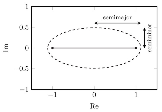
Figure 1.
The Bernstein ellipse. Its size is equal to the sum of its semiminor and semimajor axes—in this case, 1.6. Its foci and 1 are shown by the black dots.
In most practical applications, the integral in Equation (1) is not analytically computable. In 1D cases, the coefficients are generally approximated numerically using a Gauss quadrature rule [3]:
with being the quadrature nodes and weights of polynomial accuracy associated with w. According to [3], Section 3.6, the aliasing error on the polynomial expansion of f is given by
In essence, the aliasing error follows from the fact that the lower-order polynomials cannot be distinguished from the higher-order polynomials on a finite grid. As seen in Equation (7), it can be interpreted as the error that is introduced by using the lower-order discrete expansion of the higher-order polynomials instead of the higher-order polynomials themselves. In [3], it is mentioned that the aliasing error induced by using Formula (6) is usually of the same order as the projection error in Equation (5). Hence, the aliasing error will also benefit from a higher .
2.2. Conformally Mapped gPC
In [24], a framework was established to incorporate conformal maps into the gPC algorithm for enlarging the Bernstein ellipse, based on earlier research from [25]. Consider a map g that is conformal in an open region with subdomain , with and . This map can be used to define a new variable :
If x is a random variable, distributed according to the weight function with support , the variable after transformation will have its own weight function with support [24]:
The symbol ∘ is used to denote function composition, i.e., . By choosing in , the above equation becomes
Assuming that the orthogonal polynomials associated with w are known, the orthogonal polynomials associated with can be constructed by the Modified Chebyshev Algorithm [29]. Next, the quadrature points and associated weights of can be calculated using the Golub–Welsch Algorithm [30]. The Modified Chebyshev Algorithm is based upon a set of integrals called the modified moments, defined by
Only for select combinations of weight function and conformal map can these integrals be calculated analytically. In other cases, one has to make use of quadrature rules (or other computational methods) to evaluate these integrals numerically. As the quadrature nodes and weights belonging to are not yet known at this point in the algorithm, this integral has to be reformulated as an integral with weight function w, whose quadrature nodes and weights are known. One means of achieving this is by rewriting the integral as
with the quadrature nodes and weights of polynomial accuracy associated with w. Within this research, the value of was set to 50, a value for which sufficient accuracy was reached.
Instead of a polynomial expansion of f, in the conformally mapped gPC algorithm introduced by [24], an expansion of is performed, using the newly constructed polynomials:
By substituting the inverse map at both sides of Equation (12), a mapped approximation of f is obtained:
A schematic overview of this algorithm is shown in Scheme 1.
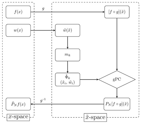
Scheme 1.
An overview of the conformally mapped gPC algorithm. A new random variable is defined by applying a conformal map on the random variable x. An adapted quadrature rule is constructed for the new weight function via the modified moments , along with its own orthogonal polynomials . Generalized Polynomial Chaos (gPC) is applied to the composite function and a mapped gPC approximation of f is found after performing the inverse conformal map .
Analogously to classic gPC, the coefficients can be approximated by means of discrete projection, yielding
with and the quadrature nodes and weights of polynomial accuracy associated with .
An upper bound similar to the one in Equation (5) can be derived for the conformally mapped gPC expansion [3,22,23,24]:
In this case, is the size of the open Bernstein ellipse , in which is analytically continuable. It is apparent from Equations (5) and (15) that the conformal map g needs to be chosen in such a way that exceeds , thus achieving a faster convergence. In other words, needs to be analytically continuable in a larger open Bernstein ellipse than f.
To the best of the authors’ knowledge, only one class of conformal map has been applied in the context of polynomial-based methods. This set of maps shifts singularities directly above or below the interval, away from the origin, in order to achieve a larger Bernstein ellipse. The Ellipse-to-Strip map [25], the Sausage map [25], the Kosloff Tal-Ezer (KTE) map [27] and the Ellipse-to-Slit map [31] all fall into this category. In Figure 2, examples are shown of these established maps.
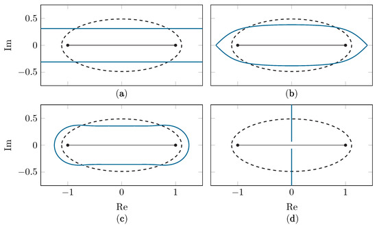
Figure 2.
The Bernstein ellipse (dashed black line) and its image (solid blue line) under the Ellipse-to-Strip map (a), the KTE map (b), the Sausage map (c) and the Ellipse-to-Slit map with slits along the imaginary axis (d).
However, it is possible to encounter function singularities in other locations of the complex plane, such as on the real axis, close to the interval. In these situations, there is a need for a new conformal map, which is proposed further in Section 2.3.
2.3. Tanh Map
Assume that f has a singularity on the real axis at location p with . Due to this singularity, the size of the Bernstein ellipse associated with f (in the x-space) is limited to . Ideally, one would use a map that gives rise to a Bernstein ellipse , associated with in the -space, that is larger than . It is clear that a suitable map for this purpose should shift the singularity away from the interval. We propose the tanh map for this purpose:
An illustration of this map for a real x and , and for different values of , is shown in Figure 3. The parameter is added to make the map adaptable to different values of the singularity’s location p.
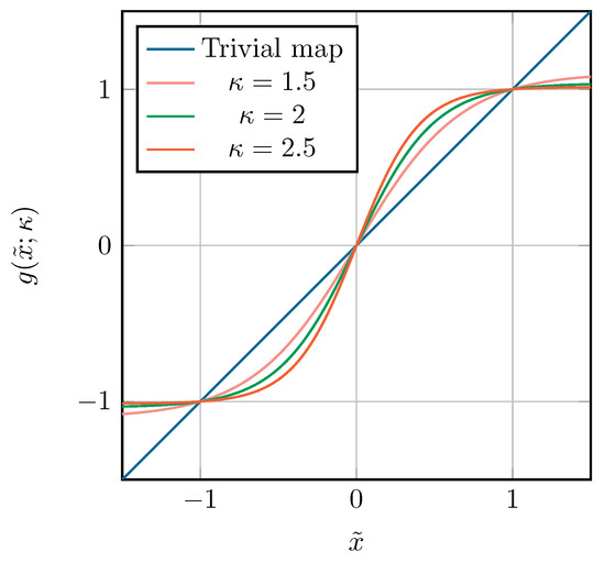
Figure 3.
The tanh map for real at different values of , together with the trivial map .
The function is periodic with period , i.e., , and has simple poles at , with . As the map needs to be bijective in order to define the inverse map, the domain of the above map is restricted to the strip around the real axis between its closest poles:
The inverse of Equation (16) can now be defined as
Using the tanh map, the singularity will shift to a position . As needs to be defined and has branch cuts and , is fundamentally limited to
Two Bernstein ellipses in the -space can be defined: one that only takes into account the shifted singularity with size
and one ellipse that only takes into account the singularities introduced by the tanh map, with size
Depending on the values of p and , either or will be the largest ellipse. As the presence of singularities is restrictive for the gPC algorithm, is equal to the size of the smallest of both ellipses, i.e., . The largest and optimal value of , named , is reached when both ellipses overlap at a certain , which can be found by solving Equations (20) and (21). Figure 4 illustrates this procedure for a singularity located at . The value of as a function of the singularity position is shown in Figure 5, along with the two regions in -space, one where and one where .
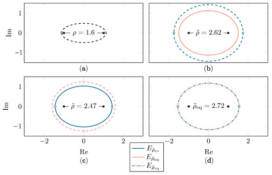
Figure 4.
The Bernstein ellipse with size (singularity located at ) in the x-space (a) and the corresponding Bernstein ellipses and when using (b), (c) and (d). The singularities are depicted with hollow dots.
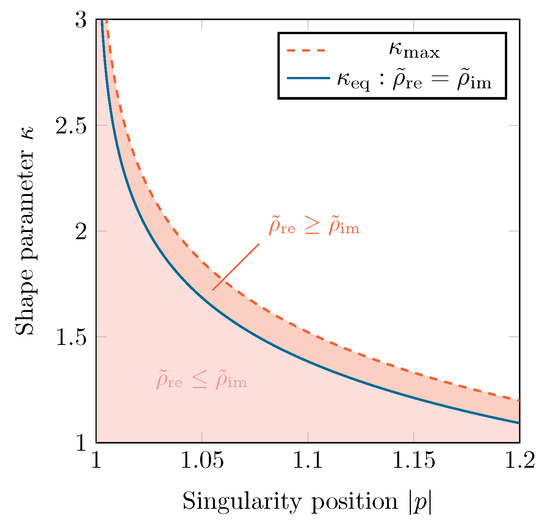
Figure 5.
The different regions, denoting the relative sizes of both Bernstein ellipses, in the -space.
Since has the singularities of g, being , on its border, it will map to an infinitely large region in the x-space, as can be seen in Figure 6. This is similar to the Ellipse-to-Strip [25] and the Ellipse-to-Slit maps [31]. The condition that f is analytically continuable within this infinite region is rather strict, and if this is not the case, the effective Bernstein ellipse will be smaller than . Luckily, the region of analyticity for f will shrink very quickly in comparison to the corresponding Bernstein ellipse . Additionally, when comparing with in Figure 7, one can conclude that, in practice, as long as singularities above and below the interval are reasonably far away, the convergence rate gain does not suffer much when applying the tanh map.
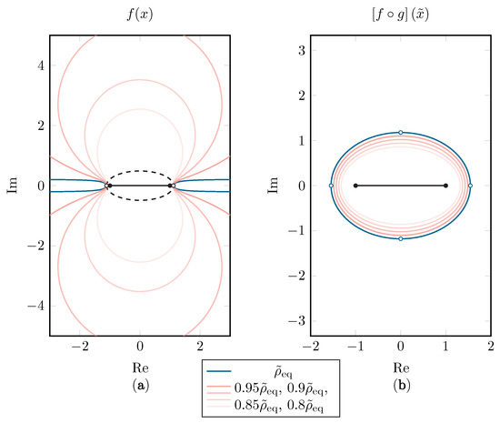
Figure 6.
Starting with a Bernstein ellipse in the x-space, the Bernstein ellipses in the -space with sizes , , , and are shown (b). The corresponding regions in which analytic continuability of f is assumed are shown in (a). The original Bernstein ellipse is shown with a dashed line as a reference and the singularities are depicted with hollow dots.
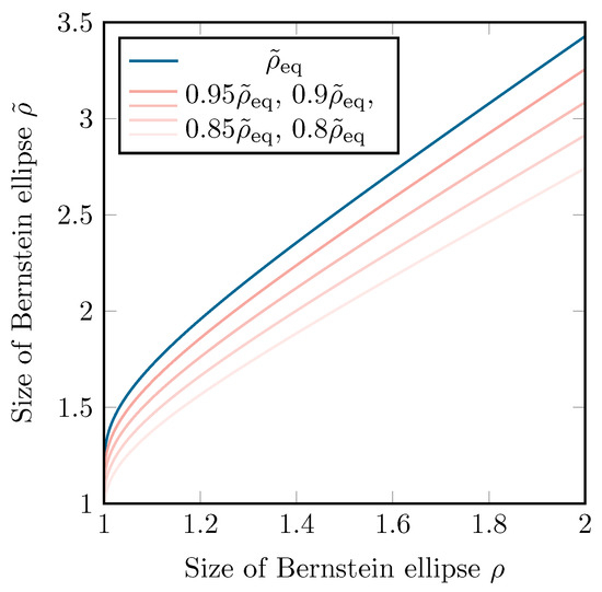
Figure 7.
The size of as a function of the size of when using the tanh map. corresponds to the maximally achievable value of .
2.4. Setup
Consider a nine-element uniform circular array (UCA) deployed in the azimuth plane. As the effects of the displacement of individual antenna elements on root-MUSIC have already been studied in earlier research—for example, in [18,19]—to showcase the proposed method, we assume that the array deforms in the shape of an ellipse with constant circumference and constant distance between the elements along the elliptical arc. This deformation is characterized by a single (random) variable: an “extended” eccentricity e defined by
with being the width of the array (along ) and the height (along ). Different array deformations are illustrated in Figure 8.
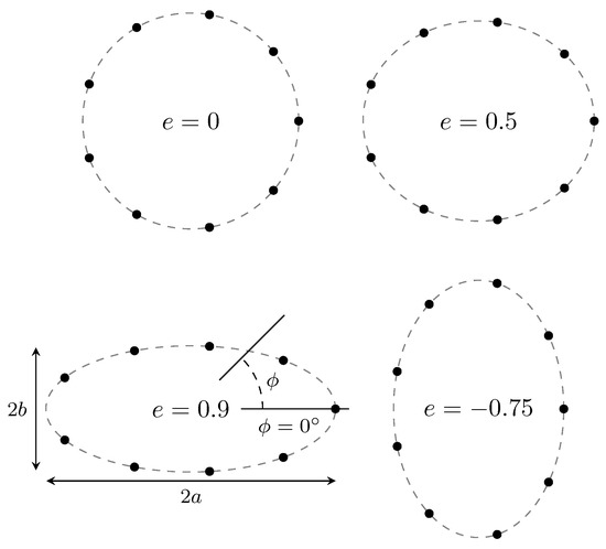
Figure 8.
The shape of the deformed UCAs for different values of e.
We limit the eccentricity to the interval , since values outside of this interval were deemed too unrealistic and the deformation would become too large for the DOA algorithm to provide a DOA estimation. However, it is standard practice [24,25] to rescale random variables to . Therefore, the random variable x is introduced as . We assume x to be distributed according to a Beta distribution [32]:
Figure 9 illustrates three Beta distributions with shape parameters , and . The orthogonal polynomials associated with the Beta distribution are the Jacobi polynomials [33].
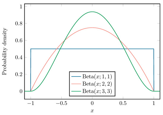
Figure 9.
The three different Beta distributions used in this work.
Since the UCA root-MUSIC algorithm was calibrated with a circular array in mind, as the array deforms, the estimated DOAs will deviate from their correct positions. This error propagation is described by a function , with being the DOA estimation corresponding to one specific source.
From a practical viewpoint, it is non-intuitive to consider the analytic continuation of in the complex plane beyond the interval. However, one can state that f, the relation between deformation and (erroneous) DOA estimation, behaves in a highly erratic manner when x approaches the edges of the interval . This behavior is equivalent to the presence of nearby singularities on the real axis. Therefore, the principles of Section 2.1, Section 2.2 and Section 2.3 apply to this case, even though has no closed form and the analytic continuation is not known.
3. Results
The operating frequency of the considered antenna array is set to 3.5 GHz (wavelength ), being the center of a 5G band [34]. The dipole elements are all of length , as is the radius of the UCA. The array is excited by six plane waves along directions , 70°, 165°, 220°, 305° and 350° in the azimuth plane. DOA estimation is performed with the UCA root-MUSIC algorithm [28]. The full-wave NEC2++ simulator [35] is applied to rigorously simulate the complete antenna array, including all mutual coupling effects. For conciseness, we only discuss the behavior of one of the six DOA estimates, being the one corresponding to the source at .
In Figure 10, Figure 11 and Figure 12, the absolute and relative errors of and are presented as a function of N for the different Beta distributions. These values are calculated with classic gPC and mapped gPC for varying values of . The expansion coefficients are approximated with discrete projection according to Equations (6) and (14). As is equal to and , the error shown in subfigures (c) is only the aliasing error introduced by the discrete projection. The error on the estimation of in subfigures (d) can, in addition to the aliasing error, be directly linked to the -error according to Equation (4). As there are no analytical solutions to compare the results with, reference values are computed numerically by means of Monte Carlo simulation, using Latin Hypercube Sampling (LHS) with samples [36]. These values are displayed in Table 1. The implemented UCA root-MUSIC algorithm has a precision of around degrees, which is why, in some graphs, convergence halts at a relative error of around and for and , respectively.
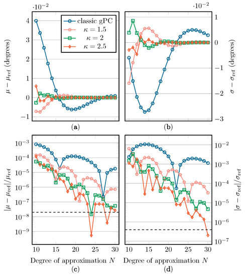
Figure 10.
The absolute and relative errors on (a,c) and (b,d) with regard to their reference value when applying the distribution. The precision floor is shown by a dashed line.
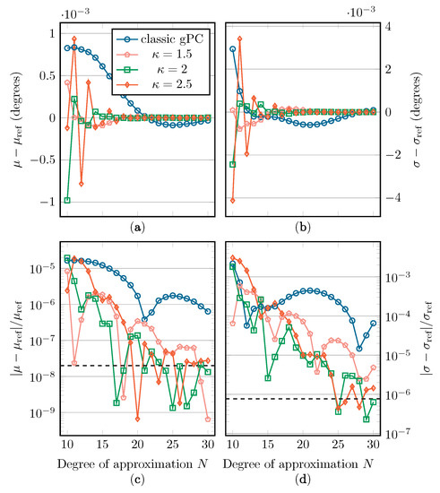
Figure 11.
The absolute and relative errors on (a,c) and (b,d) with regard to their reference value when applying the distribution. The precision floor is shown by a dashed line.
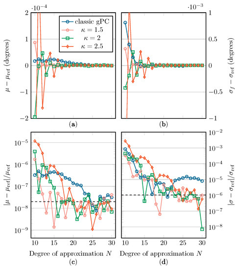
Figure 12.
The absolute and relative errors on (a,c) and (b,d) with regard to their reference value when applying the distribution. The precision floor is shown by a dashed line.

Table 1.
The reference values of and . Computed with MC using LHS and samples.
In Figure 13, a comparison between the resulting classic and mapped gPC approximations of f, using the distribution and , is shown. In Figure 14, the comparison of the resulting empirical cumulative distribution functions (CDFs) is plotted.
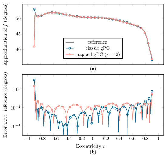
Figure 13.
(a) The approximation of f using classic and mapped gPC and (b) the error on the approximation with regard to the reference curve, with and . The reference curve was constructed by sampling the full simulation.
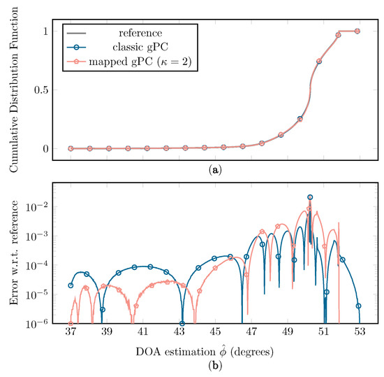
Figure 14.
(a) The empirical CDFs of when sampling the classic and mapped gPC expansion with the full simulation as a reference, each constructed with LHS and samples, with and . (b) The error of the classic and mapped gPC CDFs in comparison to the reference CDF.
4. Discussion
The discussion is presented in two parts. First, the advantages of the use of the tanh map are analyzed, based on the deformed UCA application. Afterwards, the effects of the random array deformations on the UCA root-MUSIC algorithm are discussed.
4.1. Comparison of Classic and Mapped gPC
In Figure 10, Figure 11 and Figure 12, we see a general improvement when using mapped gPC over classic gPC, as, in all cases, mapped gPC reaches the precision bound the fastest. Comparing the results for the estimation of , in subfigures (a) and (c), in which only the aliasing error is present, we can confirm that the aliasing error does indeed benefit from an increase in the size of the Bernstein ellipse. As expected, this increase in convergence rate is also present in the results for the estimation of in subfigures (b) and (d), which affirms the principles from Section 2.2 and Section 2.3. Note that the error on is linked to the -error in Equations (5) and (15) via Equation (4).
One aspect that should be mentioned is that, according to Equations (5) and (15), maximizing the size of the Bernstein ellipse only maximizes the rate of convergence, i.e., the incline of the convergence curves in subfigures (c) and (d). The vertical position of the convergence curves will, however, depend on other factors besides the size of the Bernstein ellipse. Therefore, it is possible that the fastest-converging method is not the one with the smallest error, especially in the cases with and as weight functions, where the precision floor is reached relatively quickly.
Two factors influence this phenomenon: first, the M/ parameter in Equations (5) and (15), which is an upper bound of in its supposed region of analyticity, being either for classic gPC or for mapped gPC. Although it is difficult to establish closed-form mathematical relations for the value of M/, for the mapped gPC case, one can state that an increase in will cause to either increase or stay the same, as clarified in Equation (24). In other words, an increase in convergence rate due to an increase in can be paired with an upward vertical shift in the convergence curve.
Another factor is the aliasing error, defined by Equation (7), which is a function of the used weight function w/ and the expansion polynomials /, adding a dependency on w and . An exact evaluation of Equation (7) is difficult. Upper bounds to the aliasing error are available for, among others, the Legendre and Chebychev polynomial expansions [37]; however, these are not readily applicable to this mapped gPC context. The dependency of both these factors on and w explains why we see different performance for the different values as the weight function changes, even though f and its singularities, and therefore also , stay the same. Unfortunately, it is difficult to establish closed-form mathematical relations for these dependencies.
Figure 13 shows that a better fit is achieved at the extremities of the interval when using mapped instead of classic gPC, resulting in a lower supremum error and -error. As this erratic behavior of f in these regions has a large influence on the statistical moments of the function, a better fit at the edges will have a significant impact on the accuracy of the estimation of and . Another benefit of the mapped approach is a better approximation of the CDF at the far left and far right sides, as seen in Figure 14.
4.2. Consequences for the UCA Root-MUSIC Algorithm
In the situations studied in this paper, the introduction of a random deformation of the array causes a bias in the DOA estimator of 0.05 to 0.5 degrees and a standard deviation of the DOA estimation of 1 to 2.5 degrees (depending on the distribution shape; see Table 1). All things considered, this makes the UCA root-MUSIC algorithm rather robust against the array deformations studied in this work.
5. Conclusions and Future Work
The non-polynomial behavior of the root-MUSIC DOA estimation as a function of the elliptical deformation of the UCA can be compared to the presence of singularities on the real axis, close to the interval of interest, which have a detrimental effect on the convergence of the classic gPC algorithm. Luckily, using the newly defined tanh conformal map, these singularities are moved further away from the domain of the random variable, which makes for a better characterization of the erratic behavior of the DOA estimation and, as a result, causes a considerable increase in the convergence rate of the first- and second-order statistics in comparison to classic gPC.
We conclude from the simulations that the errors induced in the DOA estimation due to the elliptical deformation of the UCA are limited to only a few degrees in most cases. However, when the eccentricity reaches an absolute value of around 0.7, the DOA estimations become very volatile, with much larger errors of up to 10 degrees.
In future work, it can be of interest to develop and research even more specific conformal maps so that each type of function singularity can be dealt with in an efficient manner. As for the DOA estimation in 5G and 6G wireless communication networks, it might be advisable to look at other types of antenna arrays, such as rectangular arrays, which are currently integrated into 5G base stations and handsets [38]. Additionally, it could be interesting to look at other, modified types of MUSIC, such as or spatial/backward/time smoothing MUSIC, which are better equipped to deal with highly correlated signals, as encountered due to multipath propagation in indoor environments [39]. The technique could also be extended to hybrid techniques, such as SpotFi, that rely on a combination of time-of-flight and angle-of-arrival with MUSIC to perform accurate localization with common WiFi infrastructures [40].
Author Contributions
S.V.B. performed the mathematical derivations, wrote the algorithm, performed the simulations and analyzed the data; S.V.B., J.V., T.V.H. and H.R. interpreted the analyzed data; S.V.B. wrote the manuscript and J.V., T.V.H. and H.R. revised it. All authors have read and agreed to the published version of the manuscript.
Funding
This work was supported by the Fonds Wetenschappelijk Onderzoek – Vlaanderen - FWO under Grants n° G0F4918N (EOS ID 30452698) and n° S001521N IoBaLeT: Sustainable Internet of
Battery-Less Things.
Institutional Review Board Statement
Not applicable.
Informed Consent Statement
Not applicable.
Data Availability Statement
Not applicable.
Conflicts of Interest
The authors declare no conflict of interest.
References
- Abbasi, Q.H.; Jilani, S.F.; Alomainy, A.; Imran, M.A. Antennas and Propagation for 5G and Beyond; Institution of Engineering and Technology: Stevenage, UK, 2020. [Google Scholar]
- Xiu, D.; Karniadakis, G.E. The Wiener—Askey polynomial chaos for stochastic differential equations. SIAM J. Sci. Comput. 2002, 24, 619–644. [Google Scholar] [CrossRef]
- Xiu, D. Numerical Methods for Stochastic Computations: A Spectral Method Approach; Princeton University Press: Princeton, NJ, USA, 2010. [Google Scholar]
- Rossi, M.; Dierck, A.; Rogier, H.; Vande Ginste, D. A stochastic framework for the variability analysis of textile antennas. IEEE Trans. Antennas Propag. 2014, 62, 6510–6514. [Google Scholar] [CrossRef] [Green Version]
- Kersaudy, P.; Mostarshedi, S.; Sudret, B.; Picon, O.; Wiart, J. Stochastic Analysis of Scattered Field by Building Facades Using Polynomial Chaos. IEEE Trans. Antennas Propag. 2014, 62, 6382–6393. [Google Scholar] [CrossRef] [Green Version]
- Rossi, M.; Stockman, G.J.; Rogier, H.; Vande Ginste, D. Stochastic Analysis of the Efficiency of a Wireless Power Transfer System Subject to Antenna Variability and Position Uncertainties. Sensors 2016, 16, 1100. [Google Scholar] [CrossRef] [Green Version]
- Du, J.; Roblin, C. Statistical modeling of disturbed antennas based on the polynomial chaos expansion. IEEE Antennas Wirel. Propag. Lett. 2016, 16, 1843–1846. [Google Scholar] [CrossRef]
- Nguyen, B.T.; Samimi, A.; Vergara, S.E.W.; Sarris, C.D.; Simpson, J.J. Analysis of electromagnetic wave propagation in variable magnetized plasma via polynomial chaos expansion. IEEE Trans. Antennas Propag. 2018, 67, 438–449. [Google Scholar] [CrossRef]
- Ding, S.; Pichon, L. Sensitivity Analysis of an Implanted Antenna within Surrounding Biological Environment. Energies 2020, 13, 996. [Google Scholar] [CrossRef] [Green Version]
- Leifsson, L.; Du, X.; Koziel, S. Efficient yield estimation of multiband patch antennas by polynomial chaos-based Kriging. Int. J. Numer. Model. Electron. Netw. Devices Fields 2020, 33, e2722. [Google Scholar] [CrossRef] [Green Version]
- Rogier, H. Generalized Gamma-Laguerre Polynomial Chaos to Model Random Bending of Wearable Antennas. IEEE Antennas Wirel. Propag. Lett. 2022, 21, 1243–1247. [Google Scholar] [CrossRef]
- Babacan, S.D.; Molina, R.; Katsaggelos, A.K. Bayesian compressive sensing using Laplace priors. IEEE Trans. Image Process. 2009, 19, 53–63. [Google Scholar] [CrossRef]
- Zhang, Z.; Batselier, K.; Liu, H.; Daniel, L.; Wong, N. Tensor computation: A new framework for high-dimensional problems in EDA. IEEE Trans. Comput.-Aided Des. Integr. Circuits Syst. 2016, 36, 521–536. [Google Scholar] [CrossRef] [Green Version]
- Salis, C.; Zygiridis, T. Dimensionality reduction of the polynomial chaos technique based on the method of moments. IEEE Antennas Wirel. Propag. Lett. 2018, 17, 2349–2353. [Google Scholar] [CrossRef]
- Kaintura, A.; Dhaene, T.; Spina, D. Review of Polynomial Chaos-Based Methods for Uncertainty Quantification in Modern Integrated Circuits. Electronics 2018, 7, 30. [Google Scholar] [CrossRef] [Green Version]
- Tomy, G.J.K.; Vinoy, K.J. A fast polynomial chaos expansion for uncertainty quantification in stochastic electromagnetic problems. IEEE Antennas Wirel. Propag. Lett. 2019, 18, 2120–2124. [Google Scholar] [CrossRef]
- Lüthen, N.; Marelli, S.; Sudret, B. Sparse polynomial chaos expansions: Literature survey and benchmark. SIAM/ASA J. Uncertain. Quantif. 2021, 9, 593–649. [Google Scholar] [CrossRef]
- Inghelbrecht, V.; Verhaevert, J.; Van Hecke, T.; Rogier, H. The influence of random element displacement on DOA estimates obtained with (Khatri–Rao-) root-MUSIC. Sensors 2014, 14, 21258–21280. [Google Scholar] [CrossRef] [Green Version]
- Inghelbrecht, V.; Verhaevert, J.; Van Hecke, T.; Rogier, H.; Moeneclaey, M.; Bruneel, H. Stochastic framework for evaluating the effect of displaced antenna elements on DOA estimation. IEEE Antennas Wirel. Propag. Lett. 2016, 16, 262–265. [Google Scholar] [CrossRef] [Green Version]
- Van der Vorst, T.; Van Eeckhaute, M.; Benlarbi-Delai, A.; Sarrazin, J.; Horlin, F.; De Doncker, P. Propagation of uncertainty in the MUSIC algorithm using polynomial chaos expansions. In Proceedings of the 11th European Conference on Antennas and Propagation, Paris, France, 19–24 March 2017; pp. 820–822. [Google Scholar]
- Van der Vorst, T.; Van Eeckhaute, M.; Benlarbi-Delai, A.; Sarrazin, J.; Quitin, F.; Horlin, F.; De Doncker, P. Application of polynomial chaos expansions for uncertainty estimation in angle-of-arrival based localization. In Uncertainty Modeling for Engineering Applications; Springer: Berlin/Heidelberg, Germany, 2019; pp. 103–117. [Google Scholar]
- Bernstein, S. Sur l’ordre de la Meilleure Approximation des Fonctions Continues par des Polynômes de Degré Donné; Hayez, Imprimeur des Académies Royales: Brussels, Belgium, 1912; Volume 4. [Google Scholar]
- Trefethen, L.N. Approximation Theory and Approximation Practice; Siam: Philadelphia, PA, USA, 2019; Volume 164. [Google Scholar]
- Georg, N.; Römer, U. Conformally mapped polynomial chaos expansions for Maxwell’s source problem with random input data. Int. J. Numer. Model. Electron. Netw. Devices Fields 2020, 33, 2776. [Google Scholar] [CrossRef]
- Hale, N.; Trefethen, L.N. New quadrature formulas from conformal maps. SIAM J. Numer. Anal. 2008, 46, 930–948. [Google Scholar] [CrossRef] [Green Version]
- Alpert, B.K. Hybrid Gauss-trapezoidal quadrature rules. SIAM J. Sci. Comput. 1999, 20, 1551–1584. [Google Scholar] [CrossRef] [Green Version]
- Kosloff, D.; Tal-Ezer, H. A modified Chebyshev pseudospectral method with an O(N-1) time step restriction. J. Comput. Phys. 1993, 104, 457–469. [Google Scholar] [CrossRef]
- Goossens, R.; Rogier, H.; Werbrouck, S. UCA Root-MUSIC with sparse uniform circular arrays. IEEE Trans. Signal Process. 2008, 56, 4095–4099. [Google Scholar] [CrossRef]
- Gautschi, W. Orthogonal polynomials—Constructive theory and applications. J. Comput. Appl. Math. 1985, 12, 61–76. [Google Scholar] [CrossRef] [Green Version]
- Golub, G.H.; Welsch, J.H. Calculation of Gauss quadrature rules. Math. Comput. 1969, 23, 221–230. [Google Scholar] [CrossRef]
- Hale, N.; Trefethen, L.N. On the Use of Conformal Maps to Speed Up Numerical Computations. Ph.D. Thesis, University of Oxford, Oxford, UK, 2009. [Google Scholar]
- Johnson, N.L.; Kotz, S.; Balakrishnan, N. Beta distributions. In Continuous Univariate Distributions, 2nd ed.; John Wiley and Sons: New York, NY, USA, 1994; pp. 221–235. [Google Scholar]
- Shen, J.; Tang, T.; Wang, L.L. Orthogonal polynomials and related approximation results. In Spectral Methods; Springer: Berlin/Heidelberg, Germany, 2011; pp. 47–140. [Google Scholar]
- Habibi, M.A.; Nasimi, M.; Han, B.; Schotten, H.D. A comprehensive survey of RAN architectures toward 5G mobile communication system. IEEE Access 2019, 7, 70371–70421. [Google Scholar] [CrossRef]
- Molteno, T.C.A.; Kyriazis, N. NEC2++: An NEC-2 Compatible Numerical Electromagnetics Code; University of Otago: Dunedin, New Zealand, 2014. [Google Scholar]
- Pebesma, E.J.; Heuvelink, G.B. Latin hypercube sampling of Gaussian random fields. Technometrics 1999, 41, 303–312. [Google Scholar] [CrossRef]
- Hesthaven, J.S.; Gottlieb, S.; Gottlieb, D. Spectral Methods for Time-Dependent Problems; Cambridge University Press: Cambridge, UK, 2007; Volume 21. [Google Scholar]
- Watanabe, A.O.; Ali, M.; Sayeed, S.Y.B.; Tummala, R.R.; Pulugurtha, M.R. A review of 5G front-end systems package integration. IEEE Trans. Compon. Packag. Manuf. Technol. 2020, 11, 118–133. [Google Scholar] [CrossRef]
- Molodtsov, V.; Kureev, A.; Khorov, E. Experimental Study of Smoothing Modifications of the MUSIC Algorithm for Direction of Arrival Estimation in Indoor Environments. IEEE Access 2021, 9, 153767–153774. [Google Scholar] [CrossRef]
- Kotaru, M.; Joshi, K.; Bharadia, D.; Katti, S. Spotfi: Decimeter level localization using wifi. In Proceedings of the 2015 ACM Conference on Special Interest Group on Data Communication, London, UK, 17–21 August 2015; pp. 269–282. [Google Scholar]
Publisher’s Note: MDPI stays neutral with regard to jurisdictional claims in published maps and institutional affiliations. |
© 2022 by the authors. Licensee MDPI, Basel, Switzerland. This article is an open access article distributed under the terms and conditions of the Creative Commons Attribution (CC BY) license (https://creativecommons.org/licenses/by/4.0/).