
Improved Dynamic Window Approach for Unmanned Surface Vehicles’ Local Path Planning Considering the Impact of Environmental Factors


Abstract
:1. Introduction
2. Method Description
2.1. Subsection
- The map (study area) was considered as an independent marine environment. Therefore, we assumed that the impact of environmental factors on USV navigation in the study area was fixed and would not change with time, and meanwhile the marine environment would not be affected by USV navigation;
- The environment map used in the study was a converted grid map composed of many small squares with a side length of 1. The free passage space and obstacles were represented with white and black separately, and then were defined as 1 and 0, respectively, in the two-dimensional array storing map information. When judging the distance, we simplified USV as a point and correspondingly modeled the square representing the obstacle into a circle with the center of this square as the center and the diameter of greater than or equal to . In this paper, the value of 1.6 was selected. In this way, the distance between the USV and the obstacle was calculated as the distance from the point to the circle;
- It was assumed that the position and speed of all obstacles on the map were obtained via the sensors and the offline map of the USV. Considering the speed and controllability of the USV, the distance threshold of obstacles was set as 200 m, so only the unknown obstacles within 200 m from USV were included in the calculation of obstacle avoidance. This method had the risk of causing the algorithm to fall into the optimal local solution, but the risk was not high in the short-distance path planning task. Thus, we saved many computing resources by this method;
- It was assumed that the given moving obstacle moved in a straight line at a uniform speed, without interaction between the environment and the obstacle;
- The USV was simplified as a point when calculating the trajectory. In addition, when calculating the collision problem, we beforehand defined the safety distance R that could reflect the size of the USV and the safety rules that were set manually. In this study, the value of R was set as 4 m;
- Since the result of a previous calculation cycle can be used as the initial condition of the current cycle in the iterative process of the algorithm, we assumed that the USV navigated according to the planned path to ensure the correctness of the subsequent calculation results. We highly support the reasonableness of this assumption given that this study fully considered the actual handling characteristics and the main environmental factors of the USV;
- There are three main marine environmental factors that can exert an impact on an USV, namely, wind, waves, and ocean currents; these can cause additive or multiplicative interference with the USV [21]. Considering the actual draft, the projected area of the USV in the air was much smaller than that under the water. Therefore, when the wind speed was less than ten m/s, the effect of wind load on the USV was usually not apparent [22], which can be ignored in path planning. Assuming that the fluid pressure only caused the wave load, its interference force and moment on the ship were caused by the fluctuation of the pressure field distribution of the fluid under the water surface [21]. Therefore, the wave load was more important in dynamic path planning than in global path planning. In reality, the ocean current was irregular and multidirectional in space and time, but this study assumed that the ocean current remained unchanged in a given time considering that the calculated sea area was small and the USV transit time was short. Since the ocean current is essentially the movement of water in the ocean, the influence of ocean currents on USVs can be expressed by the superposition of the velocity of the ocean current and the navigation velocity of the USV.
2.2. DWA Considering the Marine Environmental Impact
2.2.1. Kinematic Model
- Kinematic model in still water
- b.
- Kinematic Model Under the Influence of Wave
- c.
- Kinematic Model Under the Influence of Ocean Currents
2.2.2. Evaluation Function
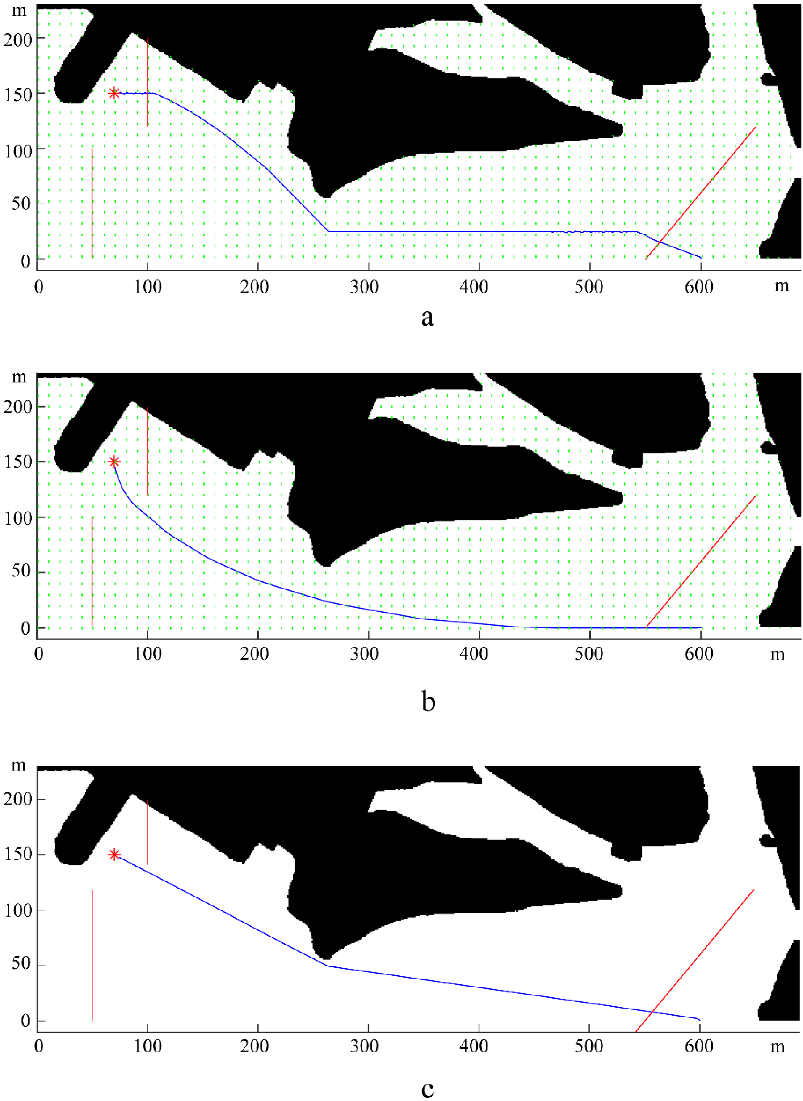
3. Simulation Results and Discussion
3.1. Simulation Results under the Action of Waves in Different Directions
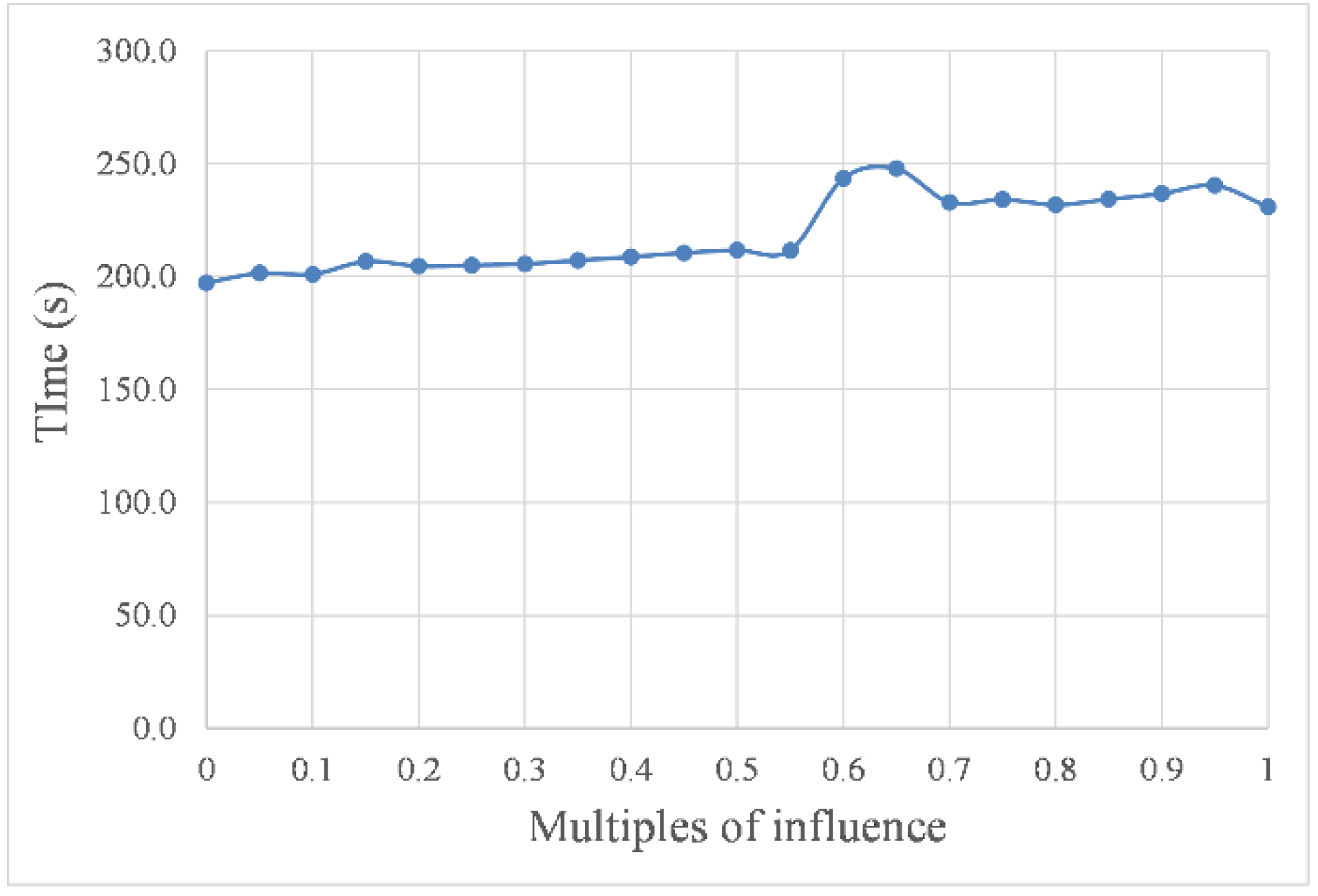
3.2. Simulation Results under the Action of Waves and Currents with Different Intensities in the Same Direction
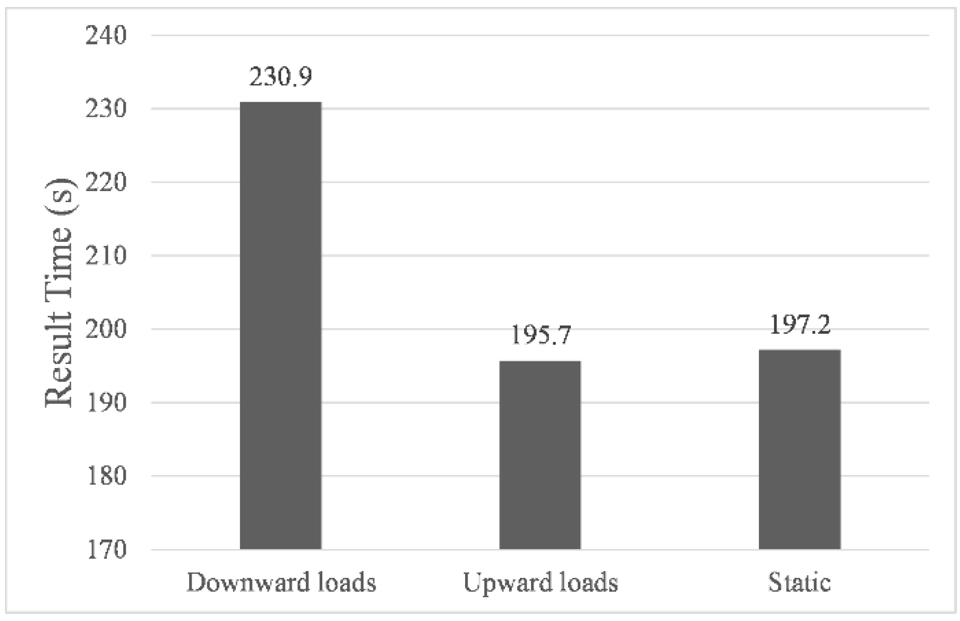
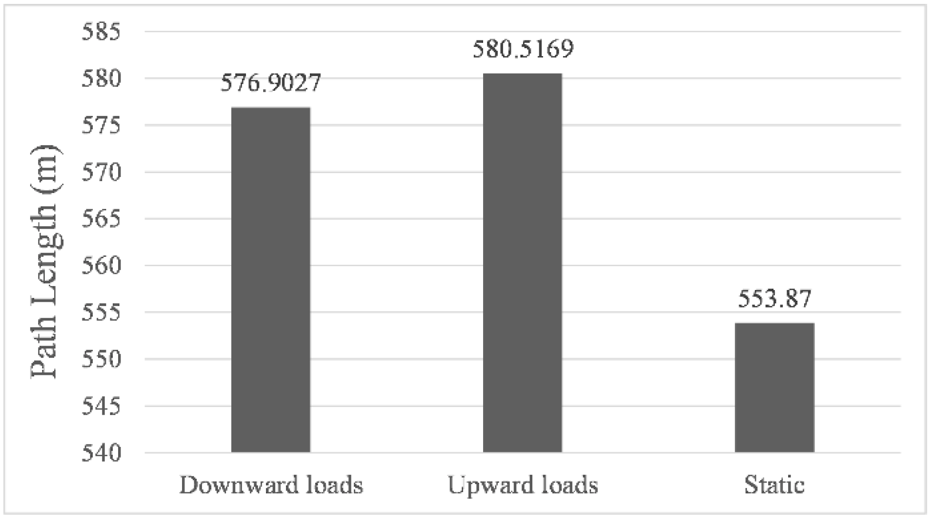
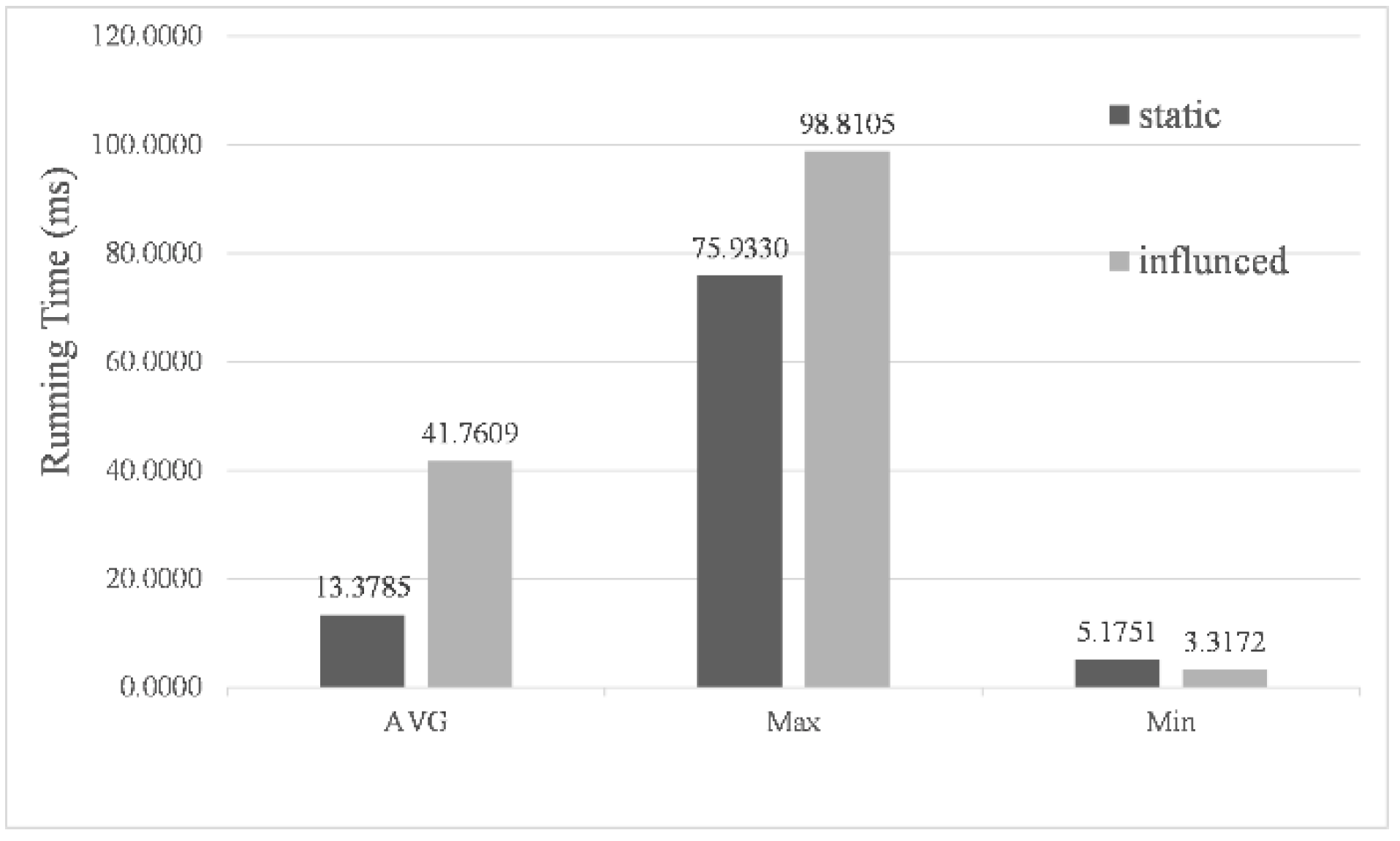
3.3. Computing Time
4. Conclusions
Author Contributions
Funding
Institutional Review Board Statement
Informed Consent Statement
Data Availability Statement
Conflicts of Interest
References
- Stateczny, A.; Specht, C.; Specht, M.; Brčić, D.; Jugović, A.; Widźgowski, S.; Wiśniewska, M.; Lewicka, O. Study on the Positioning Accuracy of GNSS/INS Systems Supported by DGPS and RTK Receivers for Hydrographic Surveys. Energies 2021, 14, 7413. [Google Scholar] [CrossRef]
- Wang, Q.; Cui, X.; Li, Y.; Ye, F. Performance Enhancement of a USV INS/CNS/DVL Integration Navigation System Based on an Adaptive Information Sharing Factor Federated Filter. Sensors 2017, 17, 239. [Google Scholar] [CrossRef] [PubMed] [Green Version]
- Xia, G.; Wang, G. INS/GNSS Tightly-Coupled Integration Using Quaternion-Based AUPF for USV. Sensors 2016, 16, 1215. [Google Scholar] [CrossRef] [PubMed] [Green Version]
- Sang, H.; You, Y.; Sun, X.; Zhou, Y.; Liu, F. The hybrid path planning algorithm based on improved A* and artificial potential field for unmanned surface vehicle formations. Ocean. Eng. 2021, 223, 108709. [Google Scholar] [CrossRef]
- Zhu, X.; Yan, B.; Yue, Y. Path Planning and Collision Avoidance in Unknown Environments for USVs Based on an Improved D* Lite. Appl. Sci. 2021, 11, 7863. [Google Scholar] [CrossRef]
- Wu, Y. Coordinated path planning for an unmanned aerial-aquatic vehicle (UAAV) and an autonomous underwater vehicle (AUV) in an underwater target strike mission. Ocean. Eng. 2019, 182, 162–173. [Google Scholar] [CrossRef]
- Sun, B.; Zhu, D.; Yang, S.X. An Optimized Fuzzy Control Algorithm for Three-Dimensional AUV Path Planning. Int. J. Fuzzy Syst. 2018, 20, 597–610. [Google Scholar] [CrossRef]
- Zeng, Z.; Sammut, K.; Lian, L.; He, F.; Lammas, A.; Tang, Y. A comparison of optimization techniques for AUV path planning in environments with ocean currents. Robot. Auton. Syst. 2016, 82, 61–72. [Google Scholar] [CrossRef]
- Singh, Y.; Sharma, S.; Sutton, R.; Hatton, D.; Khan, A. A constrained A* approach towards optimal path planning for an unmanned surface vehicle in a maritime environment containing dynamic obstacles and ocean currents. Ocean. Eng. 2018, 169, 187–201. [Google Scholar] [CrossRef] [Green Version]
- Wang, N.; Jin, X.; Er, M.J. A multilayer path planner for a USV under complex marine environments. Ocean. Eng. 2019, 184, 1–10. [Google Scholar] [CrossRef]
- Yao, Y.; Liang, X.; Li, M.; Yu, K.; Chen, Z.; Ni, C.; Teng, Y. Path Planning Method Based on D* lite Algorithm for Unmanned Surface Vehicles in Complex Environments. China Ocean. Eng. 2021, 35, 372–383. [Google Scholar] [CrossRef]
- Er, M.J.; Li, C.; Li, Q. Hybrid Adaptive Path Planning for a USV under Complex Marine Environment. In Proceedings of the 4th International Conference on Intelligent Autonomous Systems (ICoIAS), Wuhan, China, 14–16 May 2021; pp. 378–384. [Google Scholar]
- Chen, Y.; Bai, G.; Zhan, Y.; Hu, X.; Liu, J. Path Planning and Obstacle Avoiding of the USV Based on Improved ACO-APF Hybrid Algorithm with Adaptive Early-Warning. IEEE Access 2021, 9, 40728–40742. [Google Scholar] [CrossRef]
- Mousazadeh, H.; Jafarbiglu, H.; Abdolmaleki, H.; Omrani, E.; Monhaseri, F.; Abdollahzadeh, M.-R.; Mohammadi-Aghdam, A.; Kiapei, A.; Salmani-Zakaria, Y.; Makhsoos, A. Developing a navigation, guidance and obstacle avoidance algorithm for an Unmanned Surface Vehicle (USV) by algorithms fusion. Ocean. Eng. 2018, 159, 56–65. [Google Scholar] [CrossRef]
- Song, R.; Liu, Y.; Bucknall, R. A multi-layered fast marching method for unmanned surface vehicle path planning in a time-variant maritime environment. Ocean. Eng. 2017, 129, 301–317. [Google Scholar] [CrossRef]
- Ding, F.; Zhang, Z.; Fu, M.; Wang, Y.; Wang, C. Energy-Efficient Path Planning and Control Approach of USV Based on Particle Swarm Optimization. In Proceedings of the Conference on OCEANS MTS/IEEE Charleston, Charleston, SC, USA, 22–25 October 2018. [Google Scholar]
- Fang, X.; Huang, L.; Fei, Q. Path Planning Based on Improved Particle Swarm Algorithm for USV. In Proceedings of the 2021 China Automation Congress (CAC), Beijing, China, 22–24 October 2021; pp. 6918–6923. [Google Scholar]
- Tam, C.; Bucknall, R.; Greig, A. Review of Collision Avoidance and Path Planning Methods for Ships in Close Range Encounters. J. Navig. 2009, 62, 455–476. [Google Scholar] [CrossRef]
- Xiang, L.; Li, X.; Liu, H.; Li, P. Parameter Fuzzy Self-Adaptive Dynamic Window Approach for Local Path Planning of Wheeled Robot. Open J. Intell. Transp. Syst. 2022, 3, 1–6. [Google Scholar] [CrossRef]
- Jinyeong, H.; Ha, J.; Lee, J.; Ryu, J.; Yongjin, K. Dynamic Window Approach with path-following for Unmanned Surface Vehicle based on Reinforcement Learning. J. Korea Inst. Mil. Sci. Technol. 2021, 24, 61–69. [Google Scholar]
- Fossen, T.I. Guidance and Control of Ocean Vehicles; John Wiley & Sons Inc: Hoboken, NJ, USA, 1994. [Google Scholar]
- Lee, T.; Kim, H.; Chung, H.; Bang, Y.; Myung, H. Energy efficient path planning for a marine surface vehicle considering heading angle. Ocean. Eng. 2015, 107, 118–131. [Google Scholar] [CrossRef]
- Kim, H.-G.; Yun, S.-J.; Choi, Y.-H.; Ryu, J.-K.; Suh, J.-H. Collision Avoidance Algorithm Based on COLREGs for Unmanned Surface Vehicle. J. Mar. Sci. Eng. 2021, 9, 863. [Google Scholar] [CrossRef]
- Kim, H.; Yun, S.-J.; Choi, Y.-H.; Ryu, J.-K.; Won, B.-J.; Suh, J.-H. Improved Dynamic Window Approach with Ellipse Equations for Autonomous Navigation of Unmanned Surface Vehicle. J. Inst. Control. Robot. Syst. 2020, 26, 624–629. [Google Scholar] [CrossRef]
- Do, K.D.; Pan, J. Control of Ships and Underwater Vehicles: Design for Underactuated and Nonlinear Marine Systems. In Control of Ships and Underwater Vehicles: Design for Underactuated and Nonlinear Marine Systems; Springer: London, UK, 2009; pp. 1–400. [Google Scholar]
- Daidola, J.C.; Graham, D.A.; Chandrash, L. A simulation program for vessel’ s maneuvering at slow speeds. In Proceedings of the Ship Technology and Research Symposium (STAR), 11th, Portland, OR, USA, 21–23 May 1986. [Google Scholar]
- Trinh, L.A.; Ekstrom, M.; Curuklu, B. Petri Net Based Navigation Planning with Dipole Field and Dynamic Window Approach for Collision Avoidance. In Proceedings of the 6th International Conference on Control, Decision and Information Technologies (CoDIT), Conservatoire Nat Arts Metiers, Paris, France, 23–26 April 2019; pp. 1013–1018. [Google Scholar]
- Teso-Fz-Betono, D.; Zulueta, E.; Fernandez-Gamiz, U.; Saenz-Aguirre, A.; Martinez, R. Predictive Dynamic Window Approach Development with Artificial Neural Fuzzy Inference Improvement. Electronics 2019, 8, 935. [Google Scholar] [CrossRef] [Green Version]
- Zeng, T.; Si, B. Mobile Robot Exploration Based on Rapidly-exploring Random Trees and Dynamic Window Approach. In Proceedings of the 5th International Conference on Control, Automation and Robotics (ICCAR), Beijing, China, 19–22 April 2019; pp. 51–57. [Google Scholar]
- Yin, W.; Zhang, Y. Statistical analysis of wind and wave features at Bohai straits. J. Dalian Marit. Univ. 2006, 4, 84–88. (In Chinese) [Google Scholar]


| Total Mass | Length | Width | Maximum Speed | Maximum Angular Speed | Acceleration Range | Angular Acceleration Range |
|---|---|---|---|---|---|---|
| 100 kg | 2.88 m | 1.30 m | 3 m/s | 360°/s | −1~2 m/s2 | −360~360°/s2 |
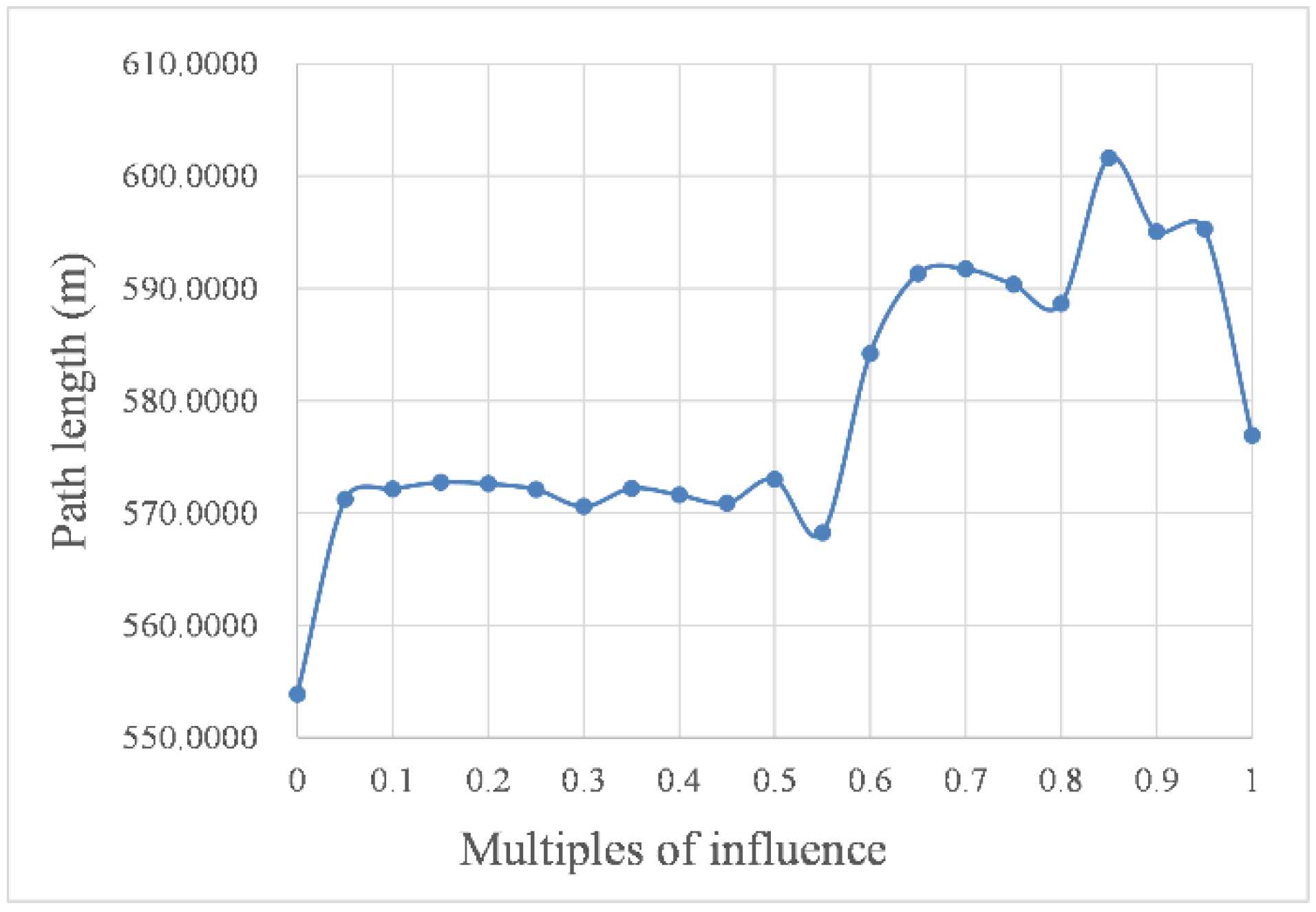
| Multiples of Intensity | Simulated Navigation Time (s) | Simulated Path Length (m) |
|---|---|---|
| 0.00 | 197.2 | 553.8700 |
| 0.05 | 201.5 | 571.2285 |
| 0.10 | 201.0 | 572.1262 |
| 0.15 | 206.7 | 573.1262 |
| 0.20 | 204.6 | 573.7434 |
| 0.25 | 205.0 | 574.7434 |
| 0.30 | 205.6 | 575.7434 |
| 0.35 | 207.2 | 576.7434 |
| 0.40 | 208.7 | 572.7434 |
| 0.45 | 210.5 | 572.7434 |
| 0.50 | 211.7 | 572.7434 |
| 0.55 | 211.6 | 564.2380 |
| 0.60 | 243.5 | 584.1969 |
| 0.65 | 247.8 | 591.3040 |
| 0.70 | 232.9 | 591.7422 |
| 0.75 | 234.2 | 590.3542 |
| 0.80 | 231.8 | 588.6524 |
| 0.85 | 234.3 | 601.6053 |
| 0.90 | 236.8 | 595.0392 |
| 0.95 | 240.4 | 595.3041 |
| 1.00 | 230.9 | 576.9027 |
Publisher’s Note: MDPI stays neutral with regard to jurisdictional claims in published maps and institutional affiliations. |
© 2022 by the authors. Licensee MDPI, Basel, Switzerland. This article is an open access article distributed under the terms and conditions of the Creative Commons Attribution (CC BY) license (https://creativecommons.org/licenses/by/4.0/).
Share and Cite
Wang, Z.; Liang, Y.; Gong, C.; Zhou, Y.; Zeng, C.; Zhu, S. Improved Dynamic Window Approach for Unmanned Surface Vehicles’ Local Path Planning Considering the Impact of Environmental Factors. Sensors 2022, 22, 5181. https://doi.org/10.3390/s22145181
Wang Z, Liang Y, Gong C, Zhou Y, Zeng C, Zhu S. Improved Dynamic Window Approach for Unmanned Surface Vehicles’ Local Path Planning Considering the Impact of Environmental Factors. Sensors. 2022; 22(14):5181. https://doi.org/10.3390/s22145181
Chicago/Turabian StyleWang, Zhenyu, Yan Liang, Changwei Gong, Yichang Zhou, Cen Zeng, and Songli Zhu. 2022. "Improved Dynamic Window Approach for Unmanned Surface Vehicles’ Local Path Planning Considering the Impact of Environmental Factors" Sensors 22, no. 14: 5181. https://doi.org/10.3390/s22145181
APA StyleWang, Z., Liang, Y., Gong, C., Zhou, Y., Zeng, C., & Zhu, S. (2022). Improved Dynamic Window Approach for Unmanned Surface Vehicles’ Local Path Planning Considering the Impact of Environmental Factors. Sensors, 22(14), 5181. https://doi.org/10.3390/s22145181