
Photoplethysmogram Recording Length: Defining Minimal Length Requirement from Dynamical Characteristics


Abstract
:1. Introduction
2. Data
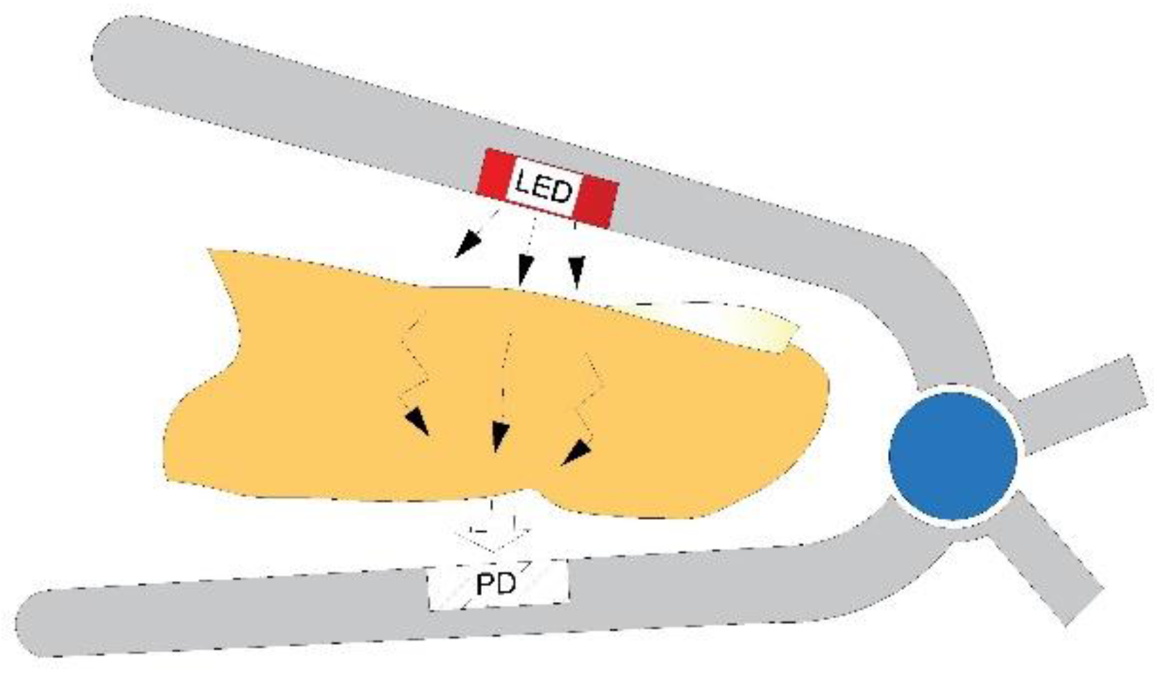
2.1. Photoplethysmogram
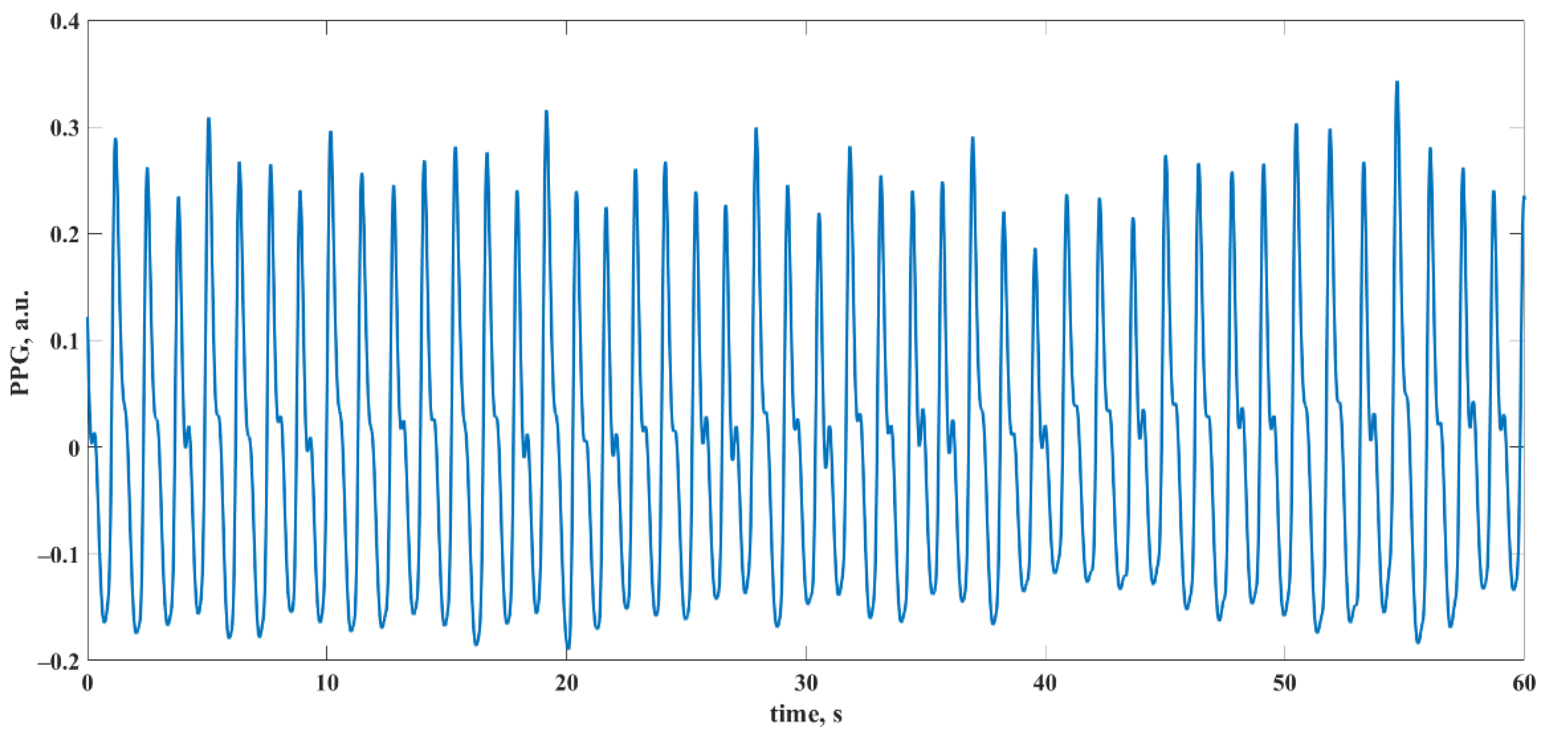
2.2. Experimental Data
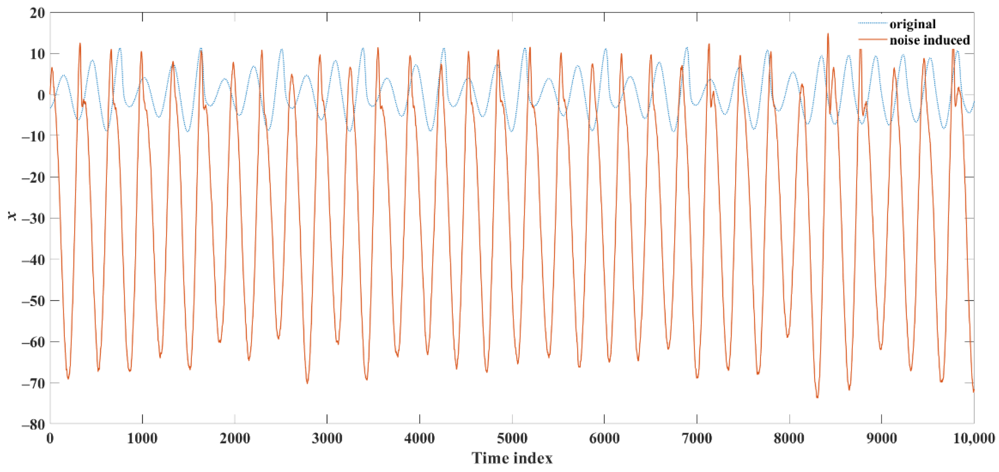
2.3. Simulated Data
3. Analysis
3.1. Time Delay Reconstruction
3.2. Recurrence Plot
3.3. Recurrence Quantification Analysis (RQA)
3.4. Error Estimation
4. Results
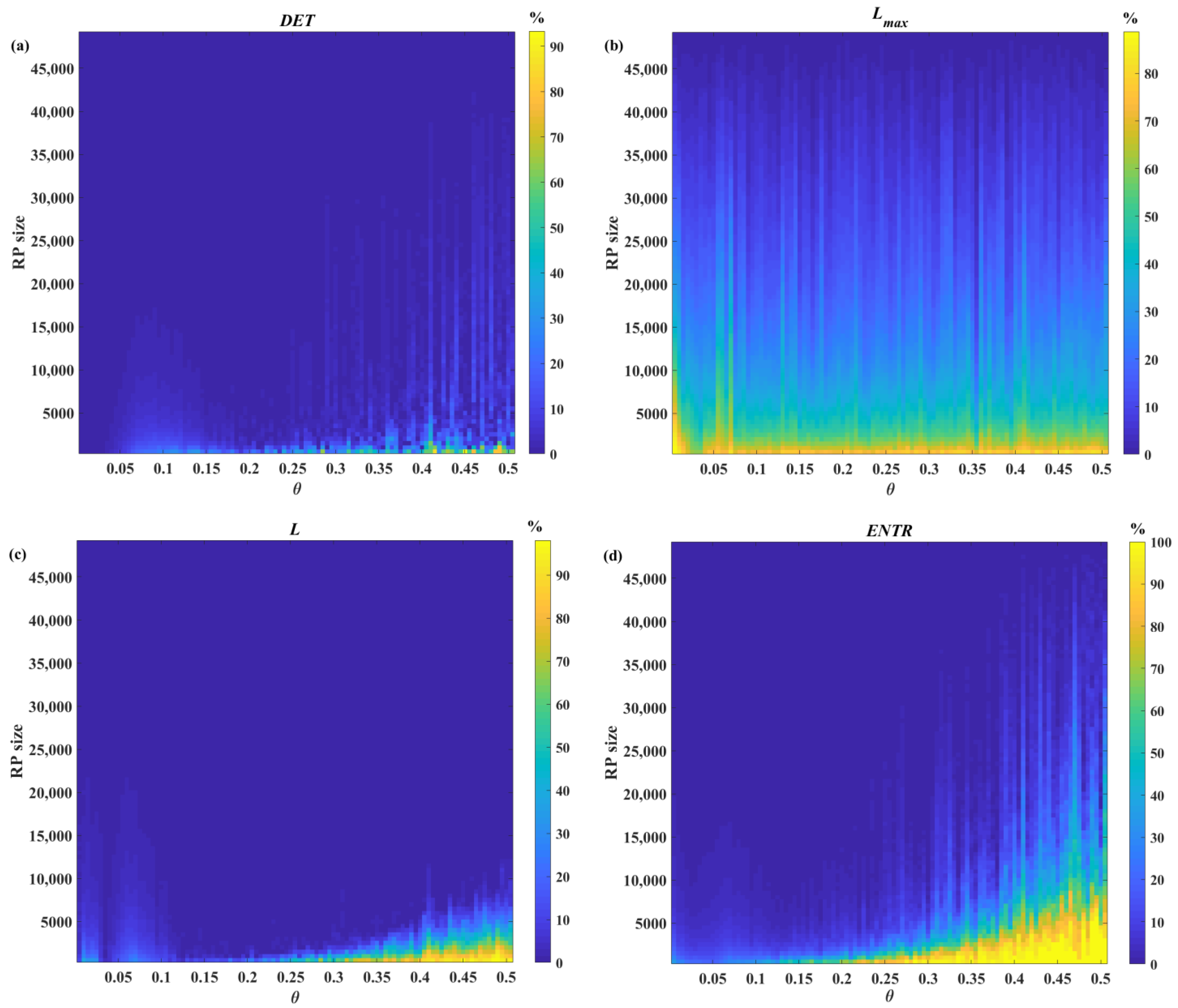
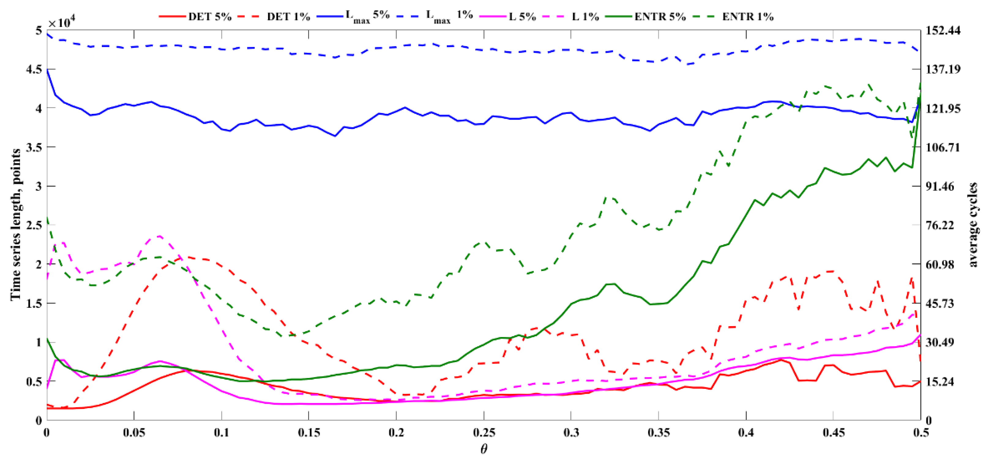
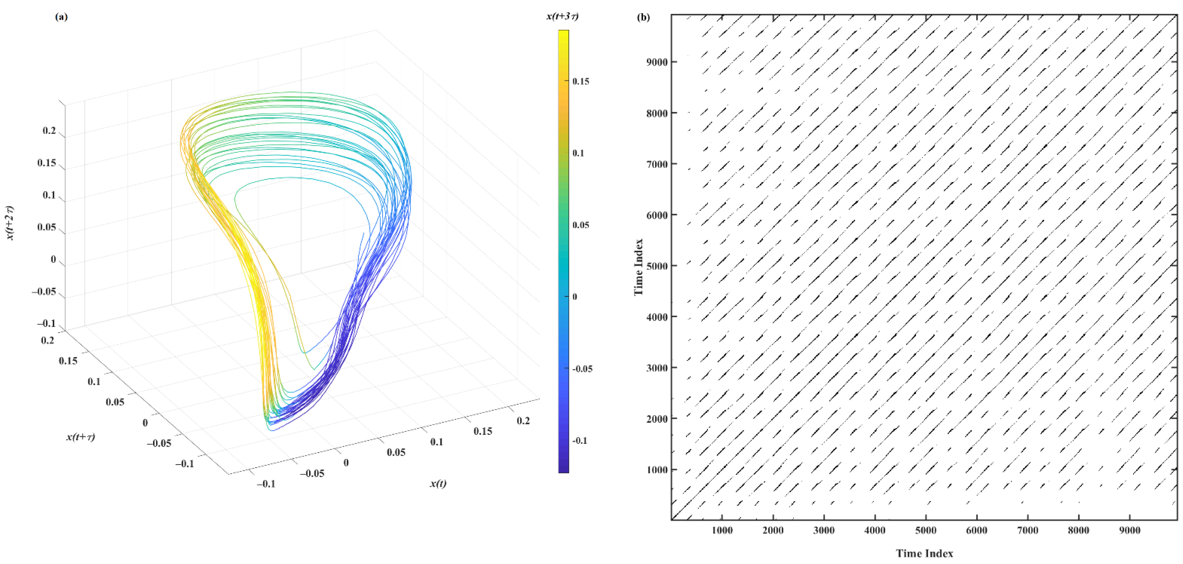
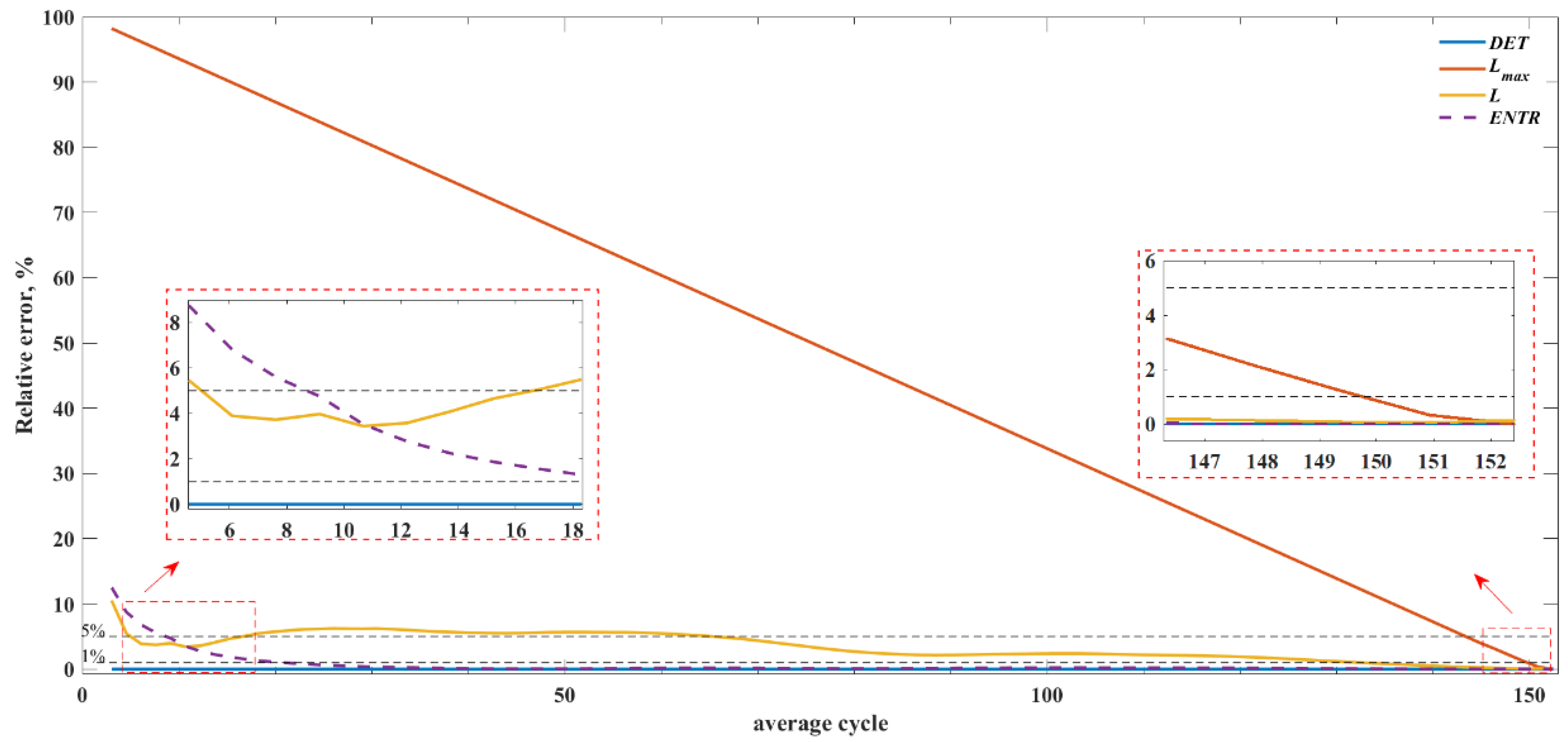
4.1. Rössler System
4.2. Photoplethysmogram
5. Discussion
6. Conclusions
Author Contributions
Funding
Institutional Review Board Statement
Informed Consent Statement
Data Availability Statement
Conflicts of Interest
References
- Cardiovascular Diseases (CVDs). Available online: https://www.who.int/news-room/fact-sheets/detail/cardiovascular-diseases-(cvds) (accessed on 5 June 2022).
- Allen, J. Photoplethysmography and Its Application in Clinical Physiological Measurement. Physiol. Meas. 2007, 28, R1–R39. [Google Scholar] [CrossRef] [PubMed] [Green Version]
- Elgendi, M. PPG Signal Analysis: An Introduction Using MATLAB; CRC Press: Boca Raton, FL, USA, 2020; ISBN 978-0-429-44958-1. [Google Scholar]
- Kyriacou, P.A. Introduction to Photoplethysmography. In Photoplethysmography; Allen, J., Kyriacou, P., Eds.; Academic Press: Cambridge, MA, USA, 2022; pp. 1–16. ISBN 978-0-12-823374-0. [Google Scholar]
- Tamura, T. Current Progress of Photoplethysmography and SPO2 for Health Monitoring. Biomed. Eng. Lett. 2019, 9, 21–36. [Google Scholar] [CrossRef] [PubMed]
- Celka, P.; Charlton, P.H.; Farukh, B.; Chowienczyk, P.; Alastruey, J. Influence of Mental Stress on the Pulse Wave Features of Photoplethysmograms. Healthc. Technol. Lett. 2019, 7, 7–12. [Google Scholar] [CrossRef] [PubMed]
- Charlton, P.H.; Celka, P.; Farukh, B.; Chowienczyk, P.; Alastruey, J. Assessing Mental Stress from the Photoplethysmogram: A Numerical Study. Physiol. Meas. 2018, 39, 054001. [Google Scholar] [CrossRef] [PubMed]
- Correia, B.; Dias, N.; Costa, P.; Pêgo, J.M. Validation of a Wireless Bluetooth Photoplethysmography Sensor Used on the Earlobe for Monitoring Heart Rate Variability Features during a Stress-Inducing Mental Task in Healthy Individuals. Sensors 2020, 20, 3905. [Google Scholar] [CrossRef] [PubMed]
- Tsuda, I.; Tahara, T.; Iwanaga, H. Chaotic Pulsation in Human Capillary Vessels and Its Dependence on Mental and Physical Conditions. Int. J. Bifurc. Chaos 1992, 2, 313–324. [Google Scholar] [CrossRef]
- Pham, T.D.; Thang, T.C.; Oyama-Higa, M.; Sugiyama, M. Mental-Disorder Detection Using Chaos and Nonlinear Dynamical Analysis of Photoplethysmographic Signals. Chaos Solitons Fractals 2013, 51, 64–74. [Google Scholar] [CrossRef]
- Sumida, T.; Arimitu, Y.; Tahara, T.; Iwanaga, H. Mental Conditions Reflected by the Chaos of Pulsation in Capillary Vessels. Int. J. Bifurc. Chaos 2000, 10, 2245–2255. [Google Scholar] [CrossRef]
- Depression. Available online: https://www.who.int/news-room/fact-sheets/detail/depression (accessed on 6 June 2022).
- Sviridova, N.; Sakai, K. Application of Photoplethysmogram for Detecting Physiological Effects of Tractor Noise. Eng. Agric. Environ. Food 2015, 8, 313–317. [Google Scholar] [CrossRef]
- Hwang, S.; Seo, J.; Jebelli, H.; Lee, S. Feasibility Analysis of Heart Rate Monitoring of Construction Workers Using a Photoplethysmography (PPG) Sensor Embedded in a Wristband-Type Activity Tracker. Autom. Constr. 2016, 71, 372–381. [Google Scholar] [CrossRef]
- Bradke, B.S.; Miller, T.A.; Everman, B. Photoplethysmography behind the Ear Outperforms Electrocardiogram for Cardiovascular Monitoring in Dynamic Environments. Sensors 2021, 21, 4543. [Google Scholar] [CrossRef] [PubMed]
- Elgendi, M. On the Analysis of Fingertip Photoplethysmogram Signals. Curr. Cardiol. Rev. 2012, 8, 14–25. [Google Scholar] [CrossRef] [PubMed]
- Millasseau, S.C.; Ritter, J.M.; Takazawa, K.; Chowienczyk, P.J. Contour Analysis of the Photoplethysmographic Pulse Measured at the Finger. J. Hypertens. 2006, 24, 1449–1456. [Google Scholar] [CrossRef] [PubMed]
- Bhat, S.; Adam, M.; Hagiwara, Y.; Ng, E.Y.K. The Biophysical Parameter Measurements from Ppg Signal. J. Mech. Med. Biol. 2017, 17, 1740005. [Google Scholar] [CrossRef]
- Kumar, A.K.; Ritam, M.; Han, L.; Guo, S.; Chandra, R. Deep Learning for Predicting Respiratory Rate from Biosignals. Comput. Biol. Med. 2022, 144, 105338. [Google Scholar] [CrossRef]
- Rong, M.; Li, K. A Multi-Type Features Fusion Neural Network for Blood Pressure Prediction Based on Photoplethysmography. Biomed. Signal Process. Control. 2021, 68, 102772. [Google Scholar] [CrossRef]
- Kim, J.W.; Choi, S.-W. Normalization of Photoplethysmography Using Deep Neural Networks for Individual and Group Comparison. Sci. Rep. 2022, 12, 3133. [Google Scholar] [CrossRef]
- Small, M.; Judd, K.; Lowe, M.; Stick, S. Is Breathing in Infants Chaotic? Dimension Estimates for Respiratory Patterns during Quiet Sleep. J. Appl. Physiol. 1999, 86, 359–376. [Google Scholar] [CrossRef] [Green Version]
- Poon, C.-S.; Merrill, C.K. Decrease of Cardiac Chaos in Congestive Heart Failure. Nature 1997, 389, 492–495. [Google Scholar] [CrossRef]
- Shelhamer, M. Nonlinear Dynamics in Physiology: A State-Space Approach; World Scientific: Singapore, 2006; ISBN 978-981-270-029-2. [Google Scholar]
- Sviridova, N.; Sakai, K. Human Photoplethysmogram: New Insight into Chaotic Characteristics. Chaos Solitons Fractals 2015, 77, 53–63. [Google Scholar] [CrossRef] [Green Version]
- Sviridova, N.; Zhao, T.; Aihara, K.; Nakamura, K.; Nakano, A. Photoplethysmogram at Green Light: Where Does Chaos Arise From? Chaos Solitons Fractals 2018, 116, 157–165. [Google Scholar] [CrossRef]
- Kaneko, K.; Tsuda, I. Complex Systems: Chaos and Beyond; Springer: Berlin/Heidelberg, Germany, 2001; ISBN 978-3-642-63132. [Google Scholar]
- Liang, Y.; Elgendi, M.; Chen, Z.; Ward, R. An Optimal Filter for Short Photoplethysmogram Signals. Sci. Data 2018, 5, 180076. [Google Scholar] [CrossRef] [PubMed]
- Ram, M.R.; Madhav, K.V.; Krishna, E.H.; Komalla, N.R.; Reddy, K.A. A Novel Approach for Motion Artifact Reduction in PPG Signals Based on AS-LMS Adaptive Filter. IEEE Trans. Instrum. Meas. 2012, 61, 1445–1457. [Google Scholar] [CrossRef]
- Peng, F.; Zhang, Z.; Gou, X.; Liu, H.; Wang, W. Motion Artifact Removal from Photoplethysmographic Signals by Combining Temporally Constrained Independent Component Analysis and Adaptive Filter. BioMed. Eng. Online 2014, 13, 50. [Google Scholar] [CrossRef] [Green Version]
- Waugh, W.; Allen, J.; Wightman, J.; Sims, A.J.; Beale, T.A.W. Novel Signal Noise Reduction Method through Cluster Analysis, Applied to Photoplethysmography. Comput. Math. Methods Med. 2018, 2018, e6812404. [Google Scholar] [CrossRef] [Green Version]
- Yan, Y.; Poon, C.C.; Zhang, Y. Reduction of Motion Artifact in Pulse Oximetry by Smoothed Pseudo Wigner-Ville Distribution. J. NeuroEng. Rehabil. 2005, 2, 3. [Google Scholar] [CrossRef] [Green Version]
- Sviridova, N. Detection of Preprocessing-Induced Changes in Chaotic Characteristics of Human Photoplethysmogram. In Proceedings of the International Symposium on Nonlinear Theory and its Applications, Kuala Lumpur, Malaysia, 2–6 December 2019; pp. 540–543. [Google Scholar]
- Badii, R.; Broggi, G.; Derighetti, B.; Ravani, M.; Ciliberto, S.; Politi, A.; Rubio, M.A. Dimension Increase in Filtered Chaotic Signals. Phys. Rev. Lett. 1988, 60, 979–982. [Google Scholar] [CrossRef]
- Liang, Y.; Chen, Z.; Liu, G.; Elgendi, M. A New, Short-Recorded Photoplethysmogram Dataset for Blood Pressure Monitoring in China. Sci. Data 2018, 5, 180020. [Google Scholar] [CrossRef] [Green Version]
- Sviridova, N.; Ikeguchi, T. Application of Recurrence Quantification Analysis to Hypertension Photoplethysmograms. In Proceedings of the International Symposium on Nonlinear Theory and Its Applications 2020, Virtual Online Conference, 16–19 November 2020; pp. 56–58. [Google Scholar]
- Sato, S.; Miao, T.; Oyama-Higa, M. Studies on Five Senses Treatment. In Knowledge-Based Systems in Biomedicine and Computational Life Science; Pham, T.D., Jain, L.C., Eds.; Studies in Computational Intelligence; Springer: Berlin/Heidelberg, Germany, 2013; pp. 155–175. ISBN 978-3-642-33015-5. [Google Scholar]
- Webber, C.L.; Zbilut, J.P. Dynamical Assessment of Physiological Systems and States Using Recurrence Plot Strategies. J. Appl. Physiol. 1994, 76, 965–973. [Google Scholar] [CrossRef]
- Marwan, N.; Carmen Romano, M.; Thiel, M.; Kurths, J. Recurrence Plots for the Analysis of Complex Systems. Phys. Rep. 2007, 438, 237–329. [Google Scholar] [CrossRef]
- Marwan, N. How to Avoid Potential Pitfalls in Recurrence Plot Based Data Analysis. Int. J. Bifurc. Chaos 2011, 21, 1003–1017. [Google Scholar] [CrossRef] [Green Version]
- Hertzman, A.B. Photoelectric Plethysmography of the Fingers and Toes in Man. Proc. Soc. Exp. Biol. Med. 1937, 37, 529–534. [Google Scholar] [CrossRef]
- Maeda, Y.; Sekine, M.; Tamura, T.; Suzuki, T.; Kameyama, K. Performance Evaluation of Green Photoplethysmography. J. Life Support Eng. 2007, 19, 183. [Google Scholar] [CrossRef]
- Maeda, Y.; Sekine, M.; Tamura, T. The Advantages of Wearable Green Reflected Photoplethysmography. J. Med. Syst. 2011, 35, 829–834. [Google Scholar] [CrossRef]
- Gagge, A.P.; Stolwijk, J.A.J.; Hardy, J.D. Comfort and Thermal Sensations and Associated Physiological Responses at Various Ambient Temperatures. Environ. Res. 1967, 1, 1–20. [Google Scholar] [CrossRef]
- Přibil, J.; Přibilová, A.; Frollo, I. Comparison of Three Prototypes of PPG Sensors for Continual Real-Time Measurement in Weak Magnetic Field. Sensors 2022, 22, 3769. [Google Scholar] [CrossRef]
- Leitner, J.; Chiang, P.-H.; Dey, S. Personalized Blood Pressure Estimation Using Photoplethysmography: A Transfer Learning Approach. IEEE J. Biomed. Health Inform. 2022, 26, 218–228. [Google Scholar] [CrossRef]
- Sviridova, N.; Sawada, K.; Ikeguchi, T. Consistency of Determinism Detection in Sparse Photoplethysmogram Recordings. In Proceedings of the BIBE2022: The Sixth International Conference on Biological Information and Biomedical Engineering, Online, 19–20 July 2022; pp. 1–4. [Google Scholar]
- Rössler, O.E. An Equation for Continuous Chaos. Phys. Lett. A 1976, 57, 397–398. [Google Scholar] [CrossRef]
- Takens, F. Detecting Strange Attractors in Turbulence. In Dynamical Systems and Turbulence, Warwick 1980; Rand, D., Young, L.-S., Eds.; Springer: Berlin/Heidelberg, Germany, 1981; pp. 366–381. [Google Scholar]
- Sauer, T.; Yorke, J.A.; Casdagli, M. Embedology. J. Stat. Phys. 1991, 65, 579–616. [Google Scholar] [CrossRef]
- Kennel, M.B.; Brown, R.; Abarbanel, H.D.I. Determining Embedding Dimension for Phase-Space Reconstruction Using a Geometrical Construction. Phys. Rev. A 1992, 45, 3403–3411. [Google Scholar] [CrossRef] [Green Version]
- Albano, A.M.; Muench, J.; Schwartz, C.; Mees, A.I.; Rapp, P.E. Singular-Value Decomposition and the Grassberger-Procaccia Algorithm. Phys. Rev. A 1988, 38, 3017–3026. [Google Scholar] [CrossRef] [PubMed] [Green Version]
- Thiel, M.; Romano, M.C.; Kurths, J.; Meucci, R.; Allaria, E.; Arecchi, F.T. Influence of Observational Noise on the Recurrence Quantification Analysis. Phys. D Nonlinear Phenom. 2002, 171, 138–152. [Google Scholar] [CrossRef] [Green Version]
- Anton, H.; Bivens, I.; Davis, S. Calculus, 7th ed.; Anton, H., Bivens, I., Davis, S., Eds.; John Wiley & Sons: New York, NY, USA, 2002; ISBN 978-0-471-43312-5. [Google Scholar]
- Rubenstein, D.A.; Yin, W.; Frame, M.D. Biofluid Mechanics: An Introduction to Fluid Mechanics, Macrocirculation, and Microcirculation; Academic Press: Cambridge, MA, USA, 2021; ISBN 978-0-12-818034-1. [Google Scholar]
- Baselli, G.; Cerutti, S.; Porta, A.; Signorini, M.G. Short and Long Term Non-Linear Analysis of RR Variability Series. Med. Eng. Phys. 2002, 24, 21–32. [Google Scholar] [CrossRef]


| Noise Level, θ | DET | Lmax | L | ENTR |
|---|---|---|---|---|
| 0 | 0.9992 | 3763.9 | 60.4329 | 4.6079 |
| 0.245 | 0.4138 | 7.52 | 2.3379 | 0.7544 |
| 0.5 | 0.0910 | 3.24 | 2.0455 | 0.1765 |
| Noise Level, θ | El | DET | Lmax | L | ENTR |
|---|---|---|---|---|---|
| 0 | 5% | 1500 | 46,000 | 4000 | 10,500 |
| 1% | 1500 | 48,500 | 16,000 | 26,000 | |
| 0.245 | 5% | 3000 | 36,500 | 2500 | 7500 |
| 1% | 17,000 | 46,000 | 3500 | 30,000 | |
| 0.5 | 5% | 5000 | 41,500 | 11,000 | 42,000 |
| 1% | 7000 | 47,000 | 13,500 | 43,500 |
| Lower Time Series Length Limit, Average Cycles | Reference RQA Values (409.6 Hz) | ||||||
|---|---|---|---|---|---|---|---|
| 409.6 Hz | 204.8 Hz | 102.4 Hz | |||||
| El, 5% | El, 1% | El, 5% | El, 1% | El, 5% | El, 1% | ||
| DET | 3.05 | 3.05 | 3.05 | 3.05 | 3.05 | 3.05 | 0.998 |
| Lmax | 144.82 | 149.39 | 143.38 | 150.28 | 143.39 | 150.25 | 49,859 |
| L | 65.55 | 131.10 | 64.19 | 132.79 | 64.02 | 133.02 | 144.38 |
| ENTR | 7.62 | 21.34 | 9.65 | 22.05 | 10.67 | 24.39 | 5.73 |
Publisher’s Note: MDPI stays neutral with regard to jurisdictional claims in published maps and institutional affiliations. |
© 2022 by the authors. Licensee MDPI, Basel, Switzerland. This article is an open access article distributed under the terms and conditions of the Creative Commons Attribution (CC BY) license (https://creativecommons.org/licenses/by/4.0/).
Share and Cite
Sviridova, N.; Zhao, T.; Nakano, A.; Ikeguchi, T. Photoplethysmogram Recording Length: Defining Minimal Length Requirement from Dynamical Characteristics. Sensors 2022, 22, 5154. https://doi.org/10.3390/s22145154
Sviridova N, Zhao T, Nakano A, Ikeguchi T. Photoplethysmogram Recording Length: Defining Minimal Length Requirement from Dynamical Characteristics. Sensors. 2022; 22(14):5154. https://doi.org/10.3390/s22145154
Chicago/Turabian StyleSviridova, Nina, Tiejun Zhao, Akimasa Nakano, and Tohru Ikeguchi. 2022. "Photoplethysmogram Recording Length: Defining Minimal Length Requirement from Dynamical Characteristics" Sensors 22, no. 14: 5154. https://doi.org/10.3390/s22145154
APA StyleSviridova, N., Zhao, T., Nakano, A., & Ikeguchi, T. (2022). Photoplethysmogram Recording Length: Defining Minimal Length Requirement from Dynamical Characteristics. Sensors, 22(14), 5154. https://doi.org/10.3390/s22145154