
A Novel Approach to Non-Destructive Rubber Vulcanization Monitoring by the Transient Radar Method

 ,
,  ,
,
Abstract
:1. Introduction
2. Materials and Methods
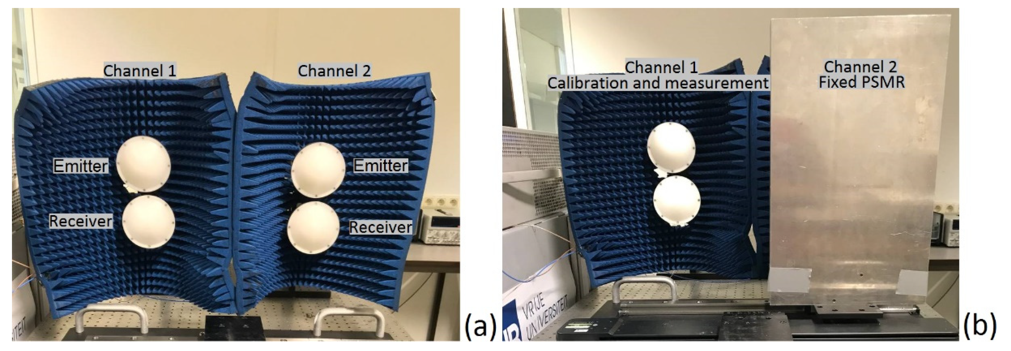
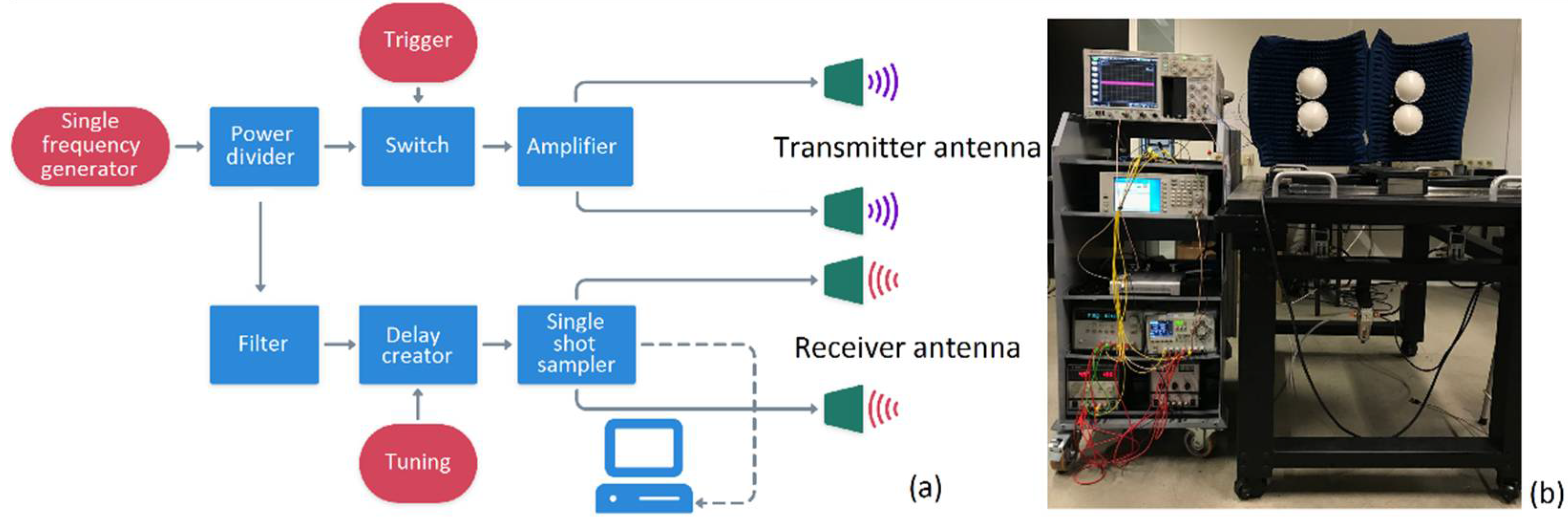
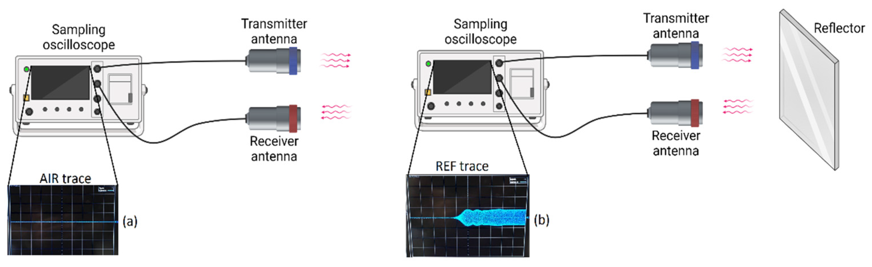
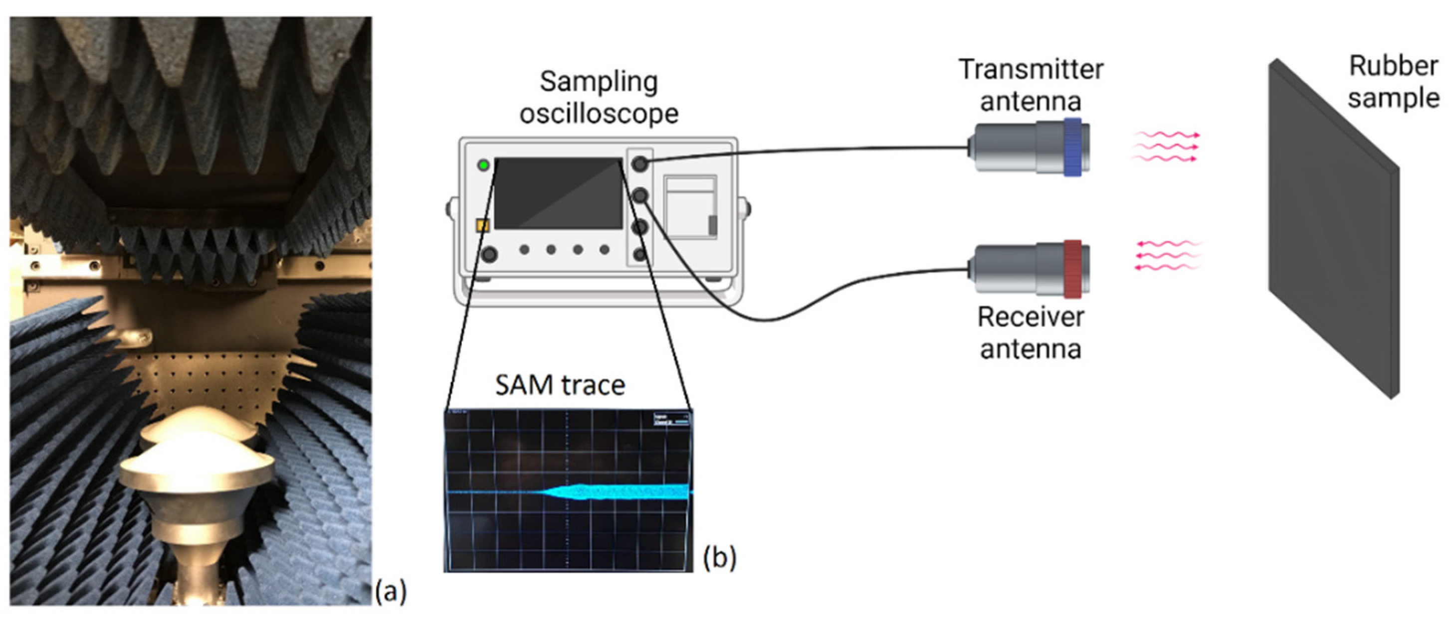
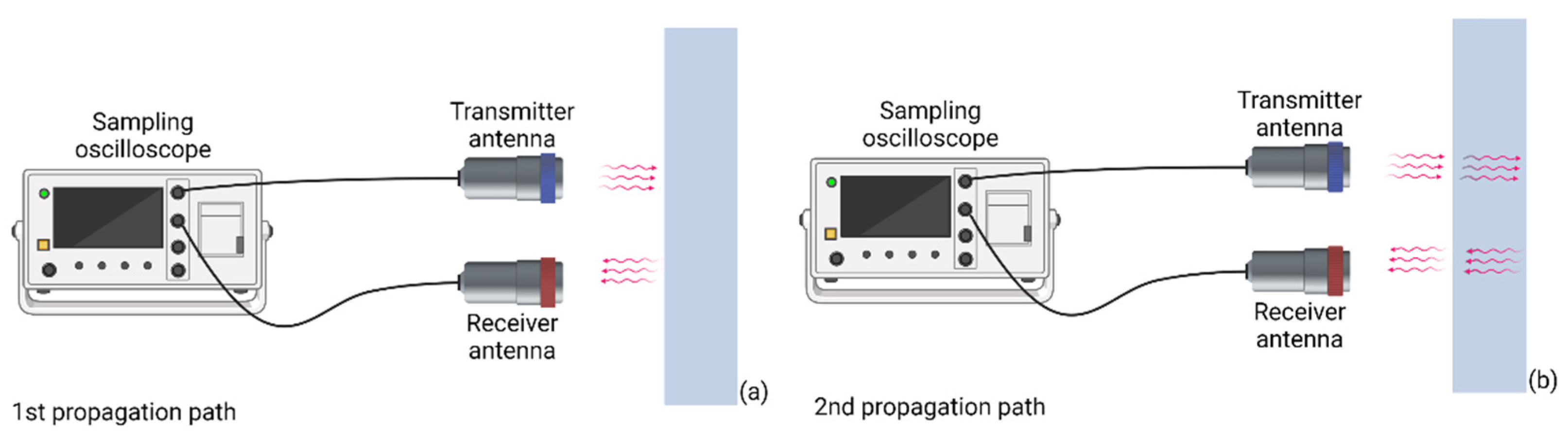
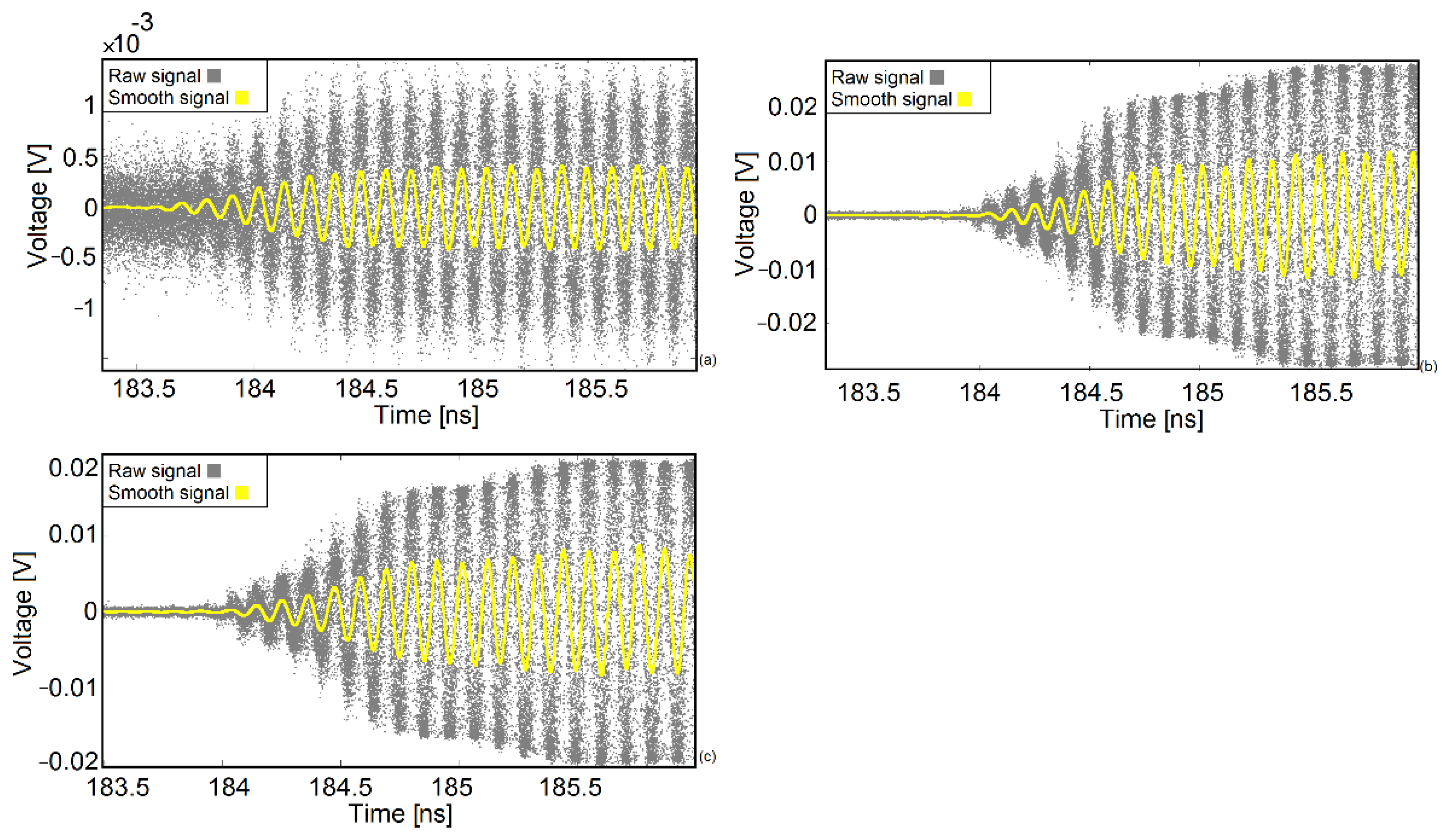
2.1. TRM System
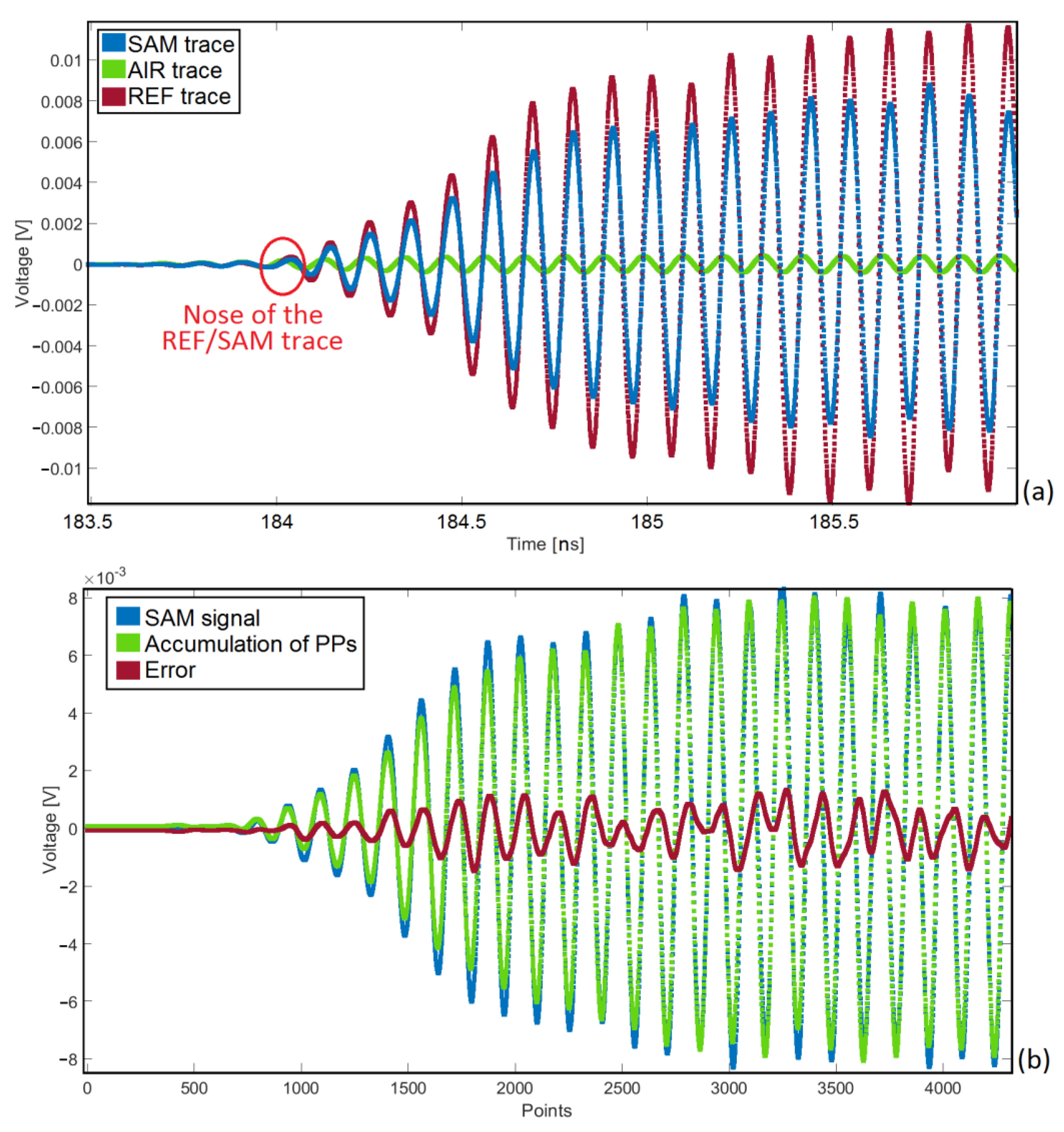
2.2. Electromagnetic and Geometric Properties Extraction
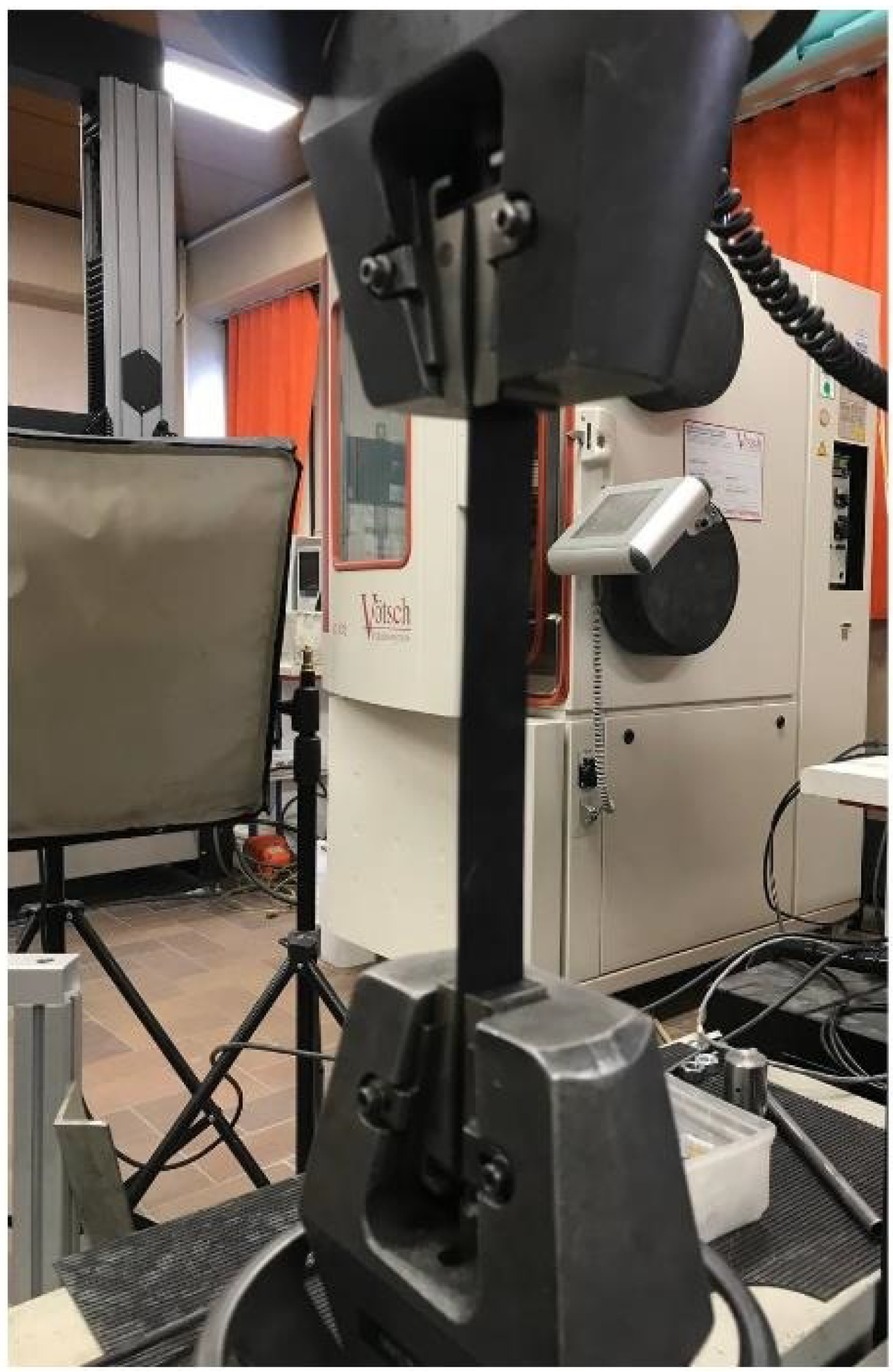
2.3. Unidirectional Tensile Test
2.4. Statistical Analyses
3. Results
3.1. Geometric and Electromagnetic Properties
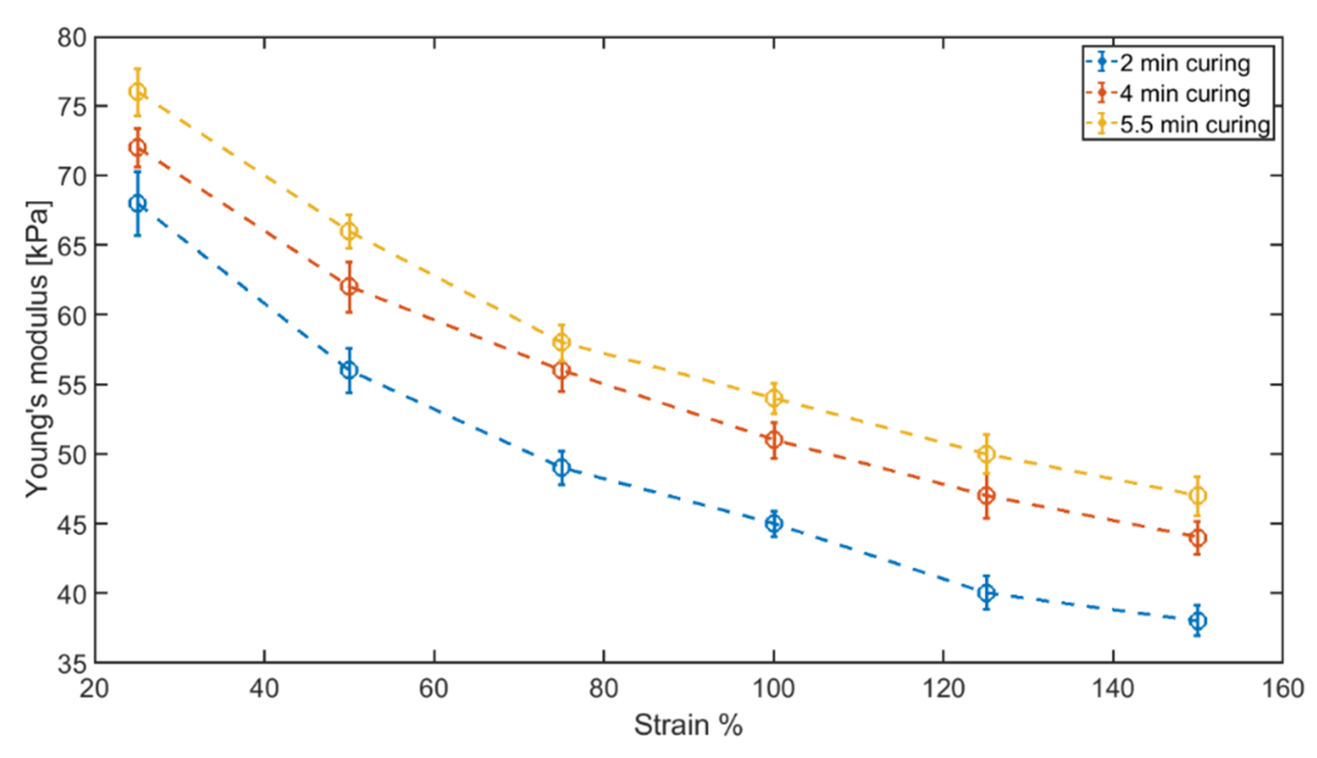
3.2. Mechanical Properties
3.3. Statistical Analyses
4. Summary and Discussion
5. Conclusions
Author Contributions
Funding
Institutional Review Board Statement
Informed Consent Statement
Data Availability Statement
Acknowledgments
Conflicts of Interest
References
- Vergnaud, J.M.; Rosca, I.D. Rubber Curing and Properties, 1st ed.; CRC Press: Boca Raton, FL, USA, 2008. [Google Scholar] [CrossRef]
- Hernández, M.; Ezquerra, A.T.; Verdejo, R.; López-Manchado, A.M. Role of Vulcanizing Additives on the Segmental Dynamics of Natural Rubber. Macromolecules 2012, 45, 1070–1075. [Google Scholar] [CrossRef] [Green Version]
- Kalia, S.; Avérous, L. Biopolymers, 1st ed.; Wiley: New York, NY, USA, 2011; Available online: https://www.perlego.com/book/1013180/biopolymers-pdf (accessed on 13 February 2022).
- Al-Sabaeei, A.M.; Yussof, N.I.; Napiah, M.B.; Sutanto, M.H. A review of using natural rubber in the modification of bitumen and asphalt mixtures used for road constuctions. J. Teknol. 2019, 81. [Google Scholar] [CrossRef]
- Borges, A.F.; Filho, E.; Miranda, M.C.R.; Santos, M.L.D.; Herculano, R.D.; Guastaldi, A.C. Natural rubber latex coated with calcium phosphate for biomedical application. J. Biomater. Sci. Polym. Ed. 2015, 26, 1256–1268. [Google Scholar] [CrossRef] [PubMed]
- Rezaeian, I.; Zahedi, P.; Rezaeian, A. Rubber Adhesion to Different Substrates and Its Importance in Industrial Applications: A Review. J. Adhes. Sci. Technol. 2012, 26, 721–744. [Google Scholar] [CrossRef]
- Mark, J.E.; Erman, B. Science and Technology of Rubber, 3rd ed.; Academic Press: Cambridge, MA, USA, 2005; ISBN 0-12-464786-3. [Google Scholar]
- Ghoreishy, M.H.R. A state-of-the-art review on the mathematical modeling and computer simulation of rubber vulcanization process. Iran. Polym. J. 2015, 25, 89–109. [Google Scholar] [CrossRef]
- El-Nemr, K.F. Effect of different curing systems on the mechanical and physico-chemical properties of acrylonitrile butadiene rubber vulcanizates. Mater. Des. 2011, 32, 3361–3369. [Google Scholar] [CrossRef]
- Chueangchayaphan, N.; Nithi-Uthai, N.; Techakittiroj, K.; Manuspiya, H. Evaluation of dielectric cure monitoring for in situ measurement of natural rubber vulcanization. Adv. Polym. Technol. 2018, 37, 3384–3391. [Google Scholar] [CrossRef]
- Zaimova, D.; Bayraktar, E.; Dishovsky, N.T. State of cure evaluation by different experimental methods in thick rubber parts. J. Achiev. Mater. Manuf. Eng. 2011, 44, 161–167. [Google Scholar]
- Rajaraian, R. Determination of Optimum Cure State of Elastomers. 2017. Available online: https://pure.mpg.de/rest/items/item_2492336/component/file_2492335/content (accessed on 26 February 2022).
- Jaunich, M.; Stark, W.; Hoster, B. Monitoring the vulcanization of elastomers: Comparison of curemeter and ultrasonic online control. Polym. Test. 2009, 28, 84–88. [Google Scholar] [CrossRef]
- Muroga, S.; Takahashi, Y.; Hikima, Y.; Ata, S.; Ohshima, M.; Okazaki, T.; Hata, K. New evaluation method for the curing degree of rubber and its nanocomposites using ATR-FTIR spectroscopy. Polym. Test 2021, 93, 106993. [Google Scholar] [CrossRef]
- Hirakawa, Y.; Yasumoto, Y.; Gondo, T.; Sone, R.; Morichika, T.; Minato, T.; Hojo, M. Application of Terahertz Spectroscopy to Rubber Products: Evaluation of Vulcanization and Silica Macro Dispersion. Electronics 2020, 9, 669. [Google Scholar] [CrossRef] [Green Version]
- Pourkazemi, A.; Stiens, J.; Becquaert, M.; Vandewal, M. Transient Radar Method: Novel Illumination and Blind Electromagnetic/Geometrical Parameter Extraction Technique for Multilayer Structures. IEEE Trans. Microw. Theory Tech. 2017, 65, 2171–2184. [Google Scholar] [CrossRef]
- Pourkazemi, A.; Tayebi, S.; Stiens, J. Fully Blind Electromagnetic Characterization of Deep Sub-Wavelength (λ/100) Dielectric Slabs With Low Bandwidth Differential Transient Radar Technique at 10 GHz. IEEE Trans. Microw. Theory Tech. 2021, 70, 1651–1657. [Google Scholar] [CrossRef]
- Pourkazemi, A.; Tayebi, S.; Stiens, J. Error Assessment and Mitigation Methods in Transient Radar Method. Sensors 2020, 20, 263. [Google Scholar] [CrossRef] [PubMed] [Green Version]


| Method | Destructive | Specific Geometry Needs | Error | Duration |
|---|---|---|---|---|
| Differential Scanning Calorimetry | Yes | None | High | <1 h |
| Mass swelling | Yes | None | Low | ≈72 h |
| Tensile test | Yes | Yes | Low | <1 h |
| Compression set test | Yes | None | Low | ≈72 h |
| Relaxation | Yes | Yes | Low | ≈1 day |
| Hardness | Yes | None | Low | <1 h |
| Shear stress | Yes | None | High | <1 h |
| Porosity | Yes | None | High | <1 h |
| THz spectroscopy | No | None | Medium | <1 h |
| ATR-FTIR spectroscopy | No | Yes | Medium | <1 h |
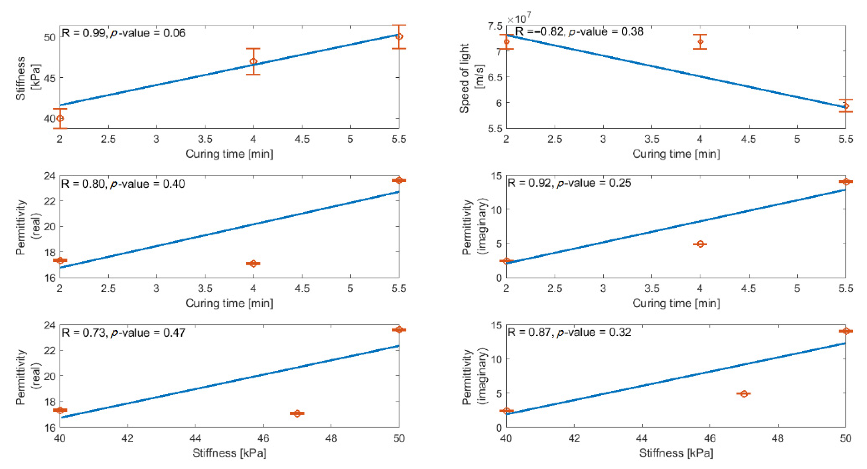
| Curing time (min) | 2.0 | 4.0 | 5.5 |
| Thickness [mm] (caliper) | 2.41 ± 0.11 | 2.21 ± 0.07 | 2.18 ± 0.15 |
| Thickness [mm] (TRM) | 2.47 ± 0.11 | 2.27 ± 0.17 | 2.36 ± 0.21 |
| Complex permittivity | 17.33 ± 0.07 − (2.41 ± 0.04)j | 17.09 ± 0.05 − (4.90 ± 0.03)j | 23.60 ± 0.05 − (14.06 ± 0.06)j |
| Relative thickness error [%] | 2.48 | 2.71 | 3.49 |
| Curing Time [min] | Young’s Modulus 25% [kPa] | Young’s Modulus 50% [kPa] | Young’s Modulus 75% [kPa] | Young’s Modulus 100% [kPa] | Young’s Modulus 125% [kPa] | Young’s Modulus 150% [kPa] |
|---|---|---|---|---|---|---|
| 2 | 68 ± 2.3 | 56 ± 1.6 | 49 ± 1.2 | 45 ± 0.9 | 40 ± 1.2 | 38 ± 1.1 |
| 4 | 72 ± 1.4 | 62 ± 1.8 | 56 ± 1.5 | 51 ± 1.3 | 47 ± 1.6 | 44 ± 1.2 |
| 5.5 | 76 ± 1.7 | 66 ± 1.2 | 58 ± 1.3 | 54 ± 1.1 | 50 ± 1.4 | 47 ± 1.4 |
Publisher’s Note: MDPI stays neutral with regard to jurisdictional claims in published maps and institutional affiliations. |
© 2022 by the authors. Licensee MDPI, Basel, Switzerland. This article is an open access article distributed under the terms and conditions of the Creative Commons Attribution (CC BY) license (https://creativecommons.org/licenses/by/4.0/).
Share and Cite
Tayebi, S.; Pourkazemi, A.; Patino, N.O.; Thibaut, K.; Kamami, O.; Stiens, J. A Novel Approach to Non-Destructive Rubber Vulcanization Monitoring by the Transient Radar Method. Sensors 2022, 22, 5010. https://doi.org/10.3390/s22135010
Tayebi S, Pourkazemi A, Patino NO, Thibaut K, Kamami O, Stiens J. A Novel Approach to Non-Destructive Rubber Vulcanization Monitoring by the Transient Radar Method. Sensors. 2022; 22(13):5010. https://doi.org/10.3390/s22135010
Chicago/Turabian StyleTayebi, Salar, Ali Pourkazemi, Nicolas Ospitia Patino, Kato Thibaut, Olsi Kamami, and Johan Stiens. 2022. "A Novel Approach to Non-Destructive Rubber Vulcanization Monitoring by the Transient Radar Method" Sensors 22, no. 13: 5010. https://doi.org/10.3390/s22135010
APA StyleTayebi, S., Pourkazemi, A., Patino, N. O., Thibaut, K., Kamami, O., & Stiens, J. (2022). A Novel Approach to Non-Destructive Rubber Vulcanization Monitoring by the Transient Radar Method. Sensors, 22(13), 5010. https://doi.org/10.3390/s22135010