
Interpolation Methods with Phase Control for Backprojection of Complex-Valued SAR Data †


Abstract
:1. Introduction
2. Problem Formulation
2.1. Notation and Conventions
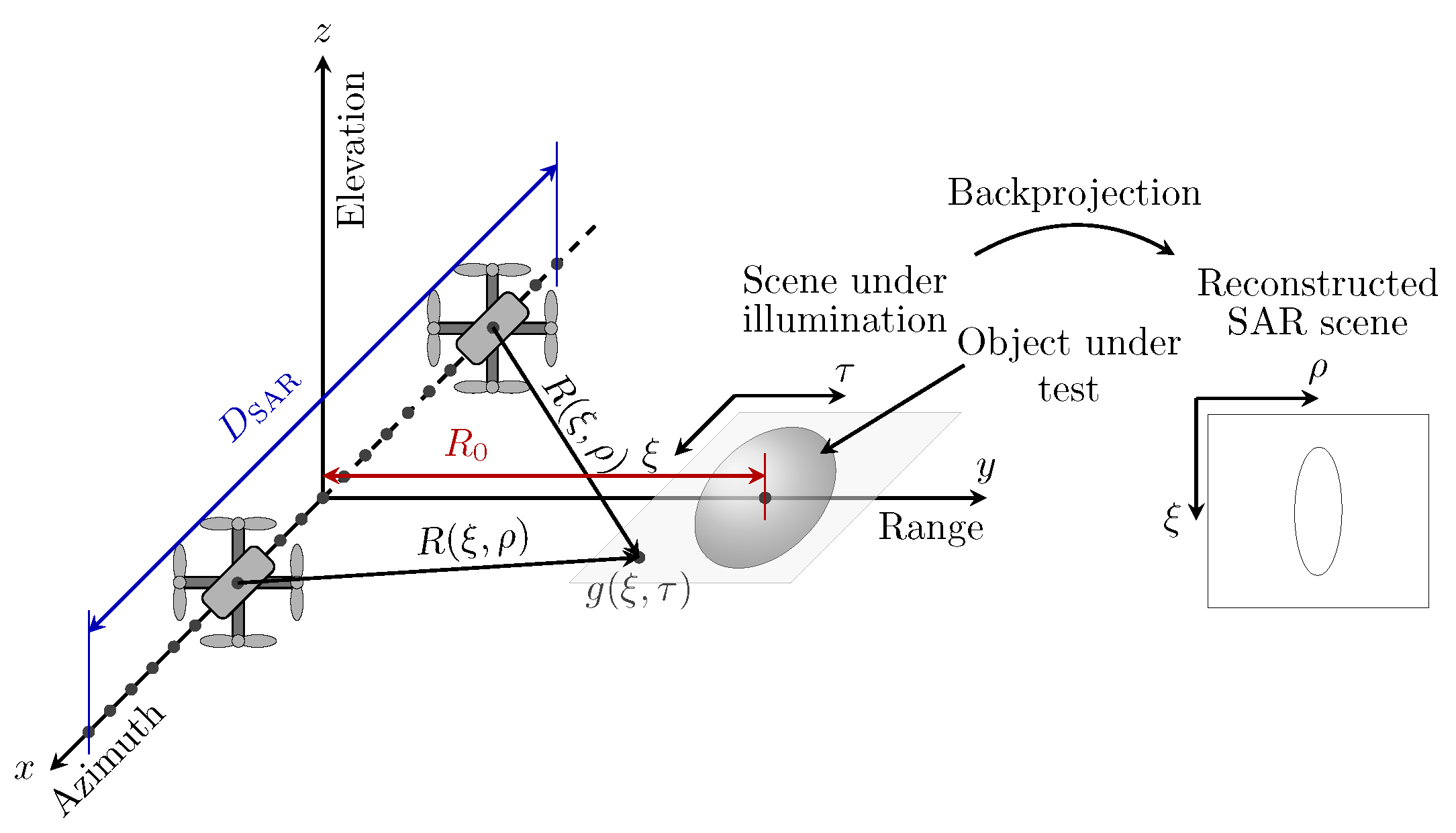
2.2. Setup
2.3. Image Formation
2.4. Phase Control of Estimated Complex SAR Data
3. Interpolation Methods
3.1. Nearest Neighbor Interpolation
3.2. Extended Linear-Spline Interpolation
3.3. Extended Cubic-Spline Interpolation
3.4. Extended Sinc Interpolation
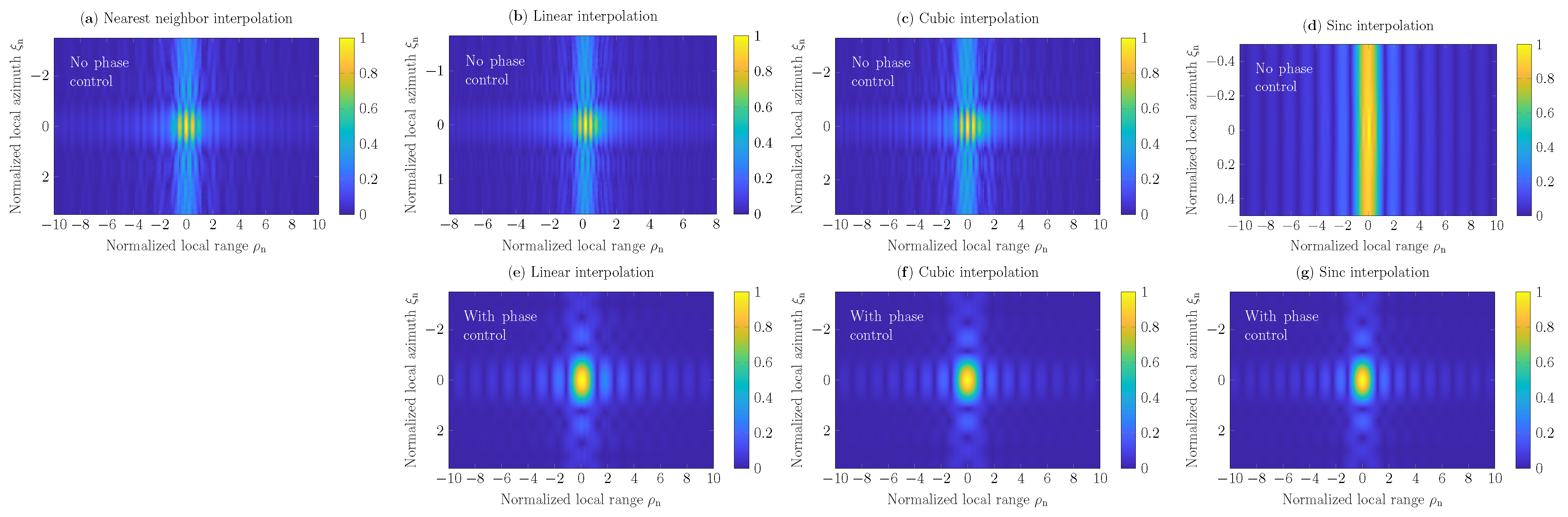
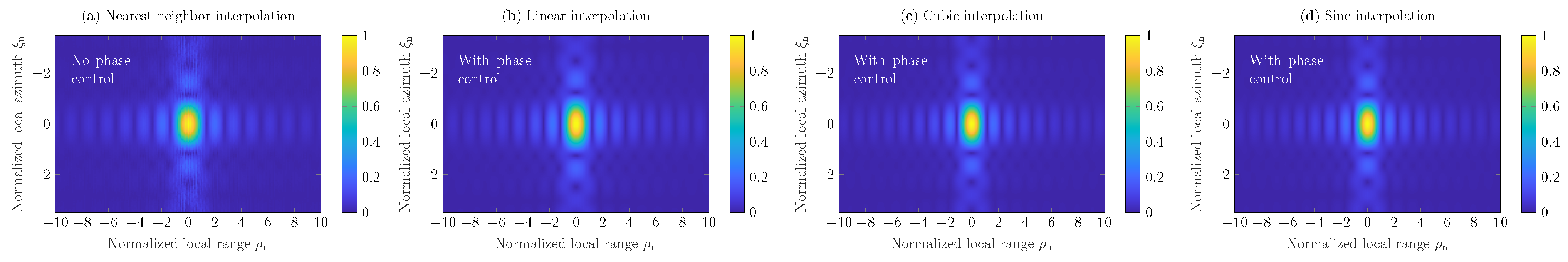
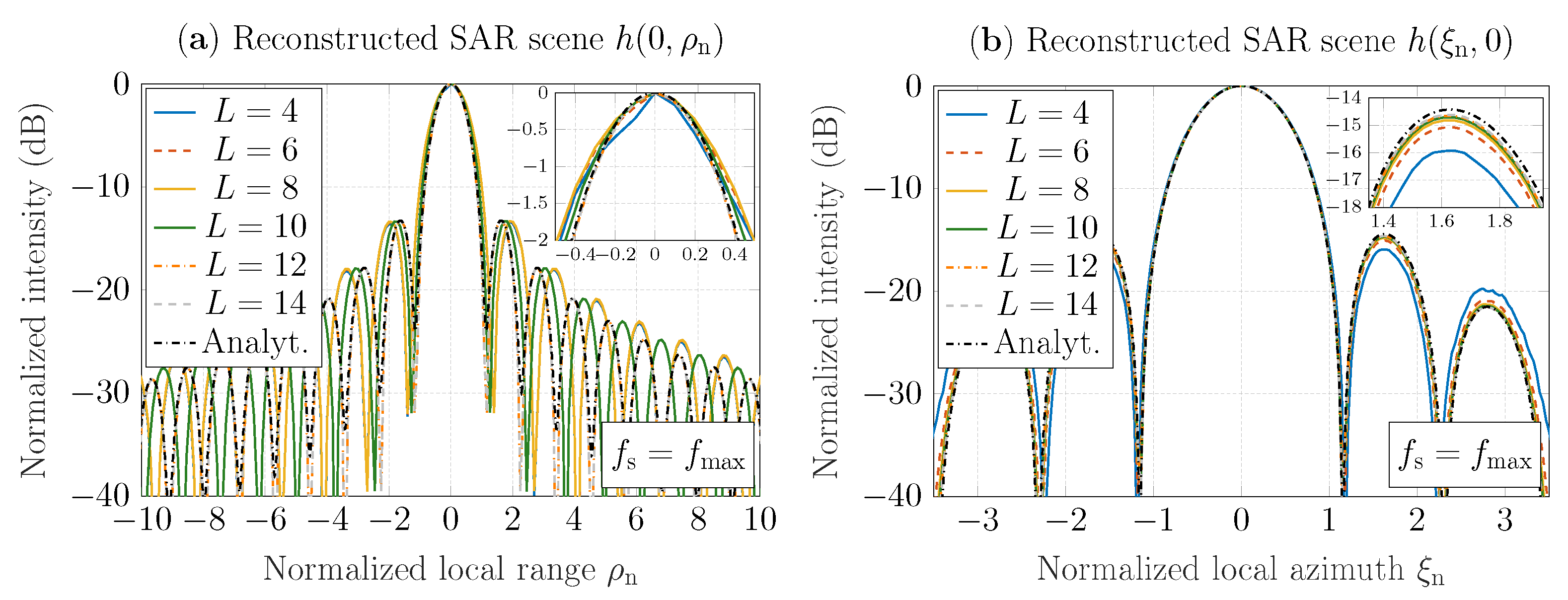
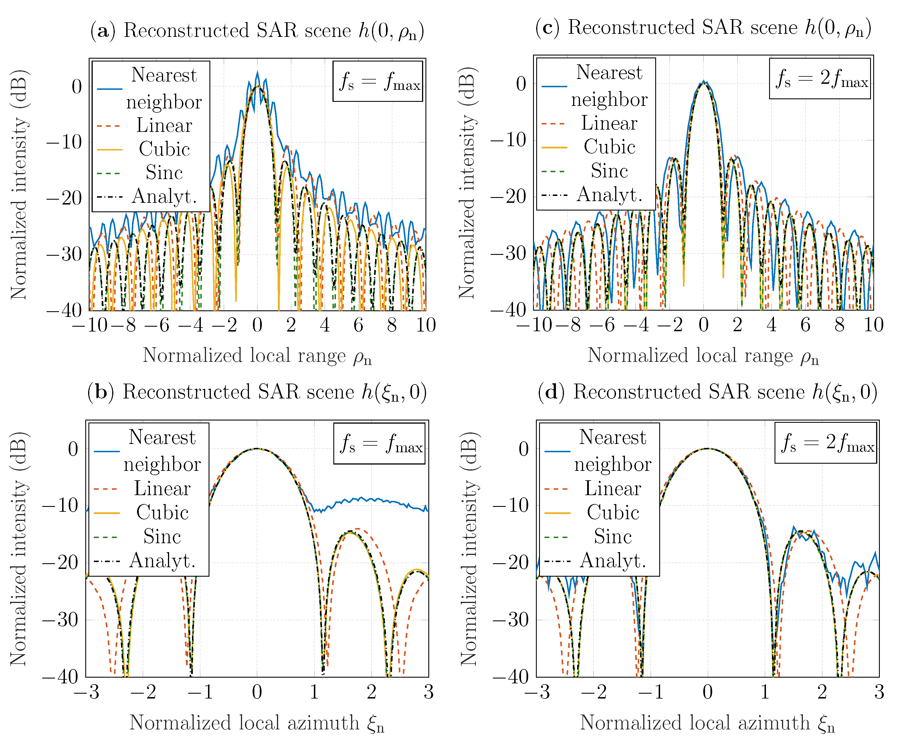
4. Simulations
4.1. Simulation Setup
4.2. Results
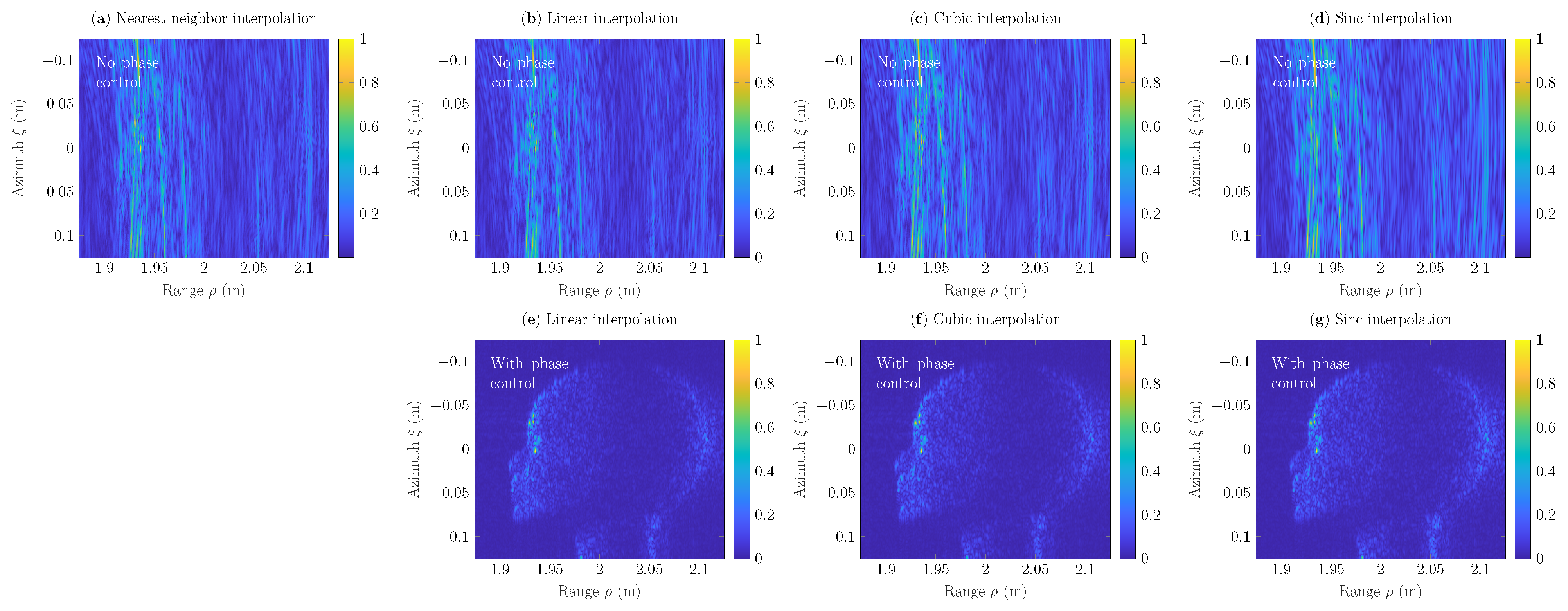
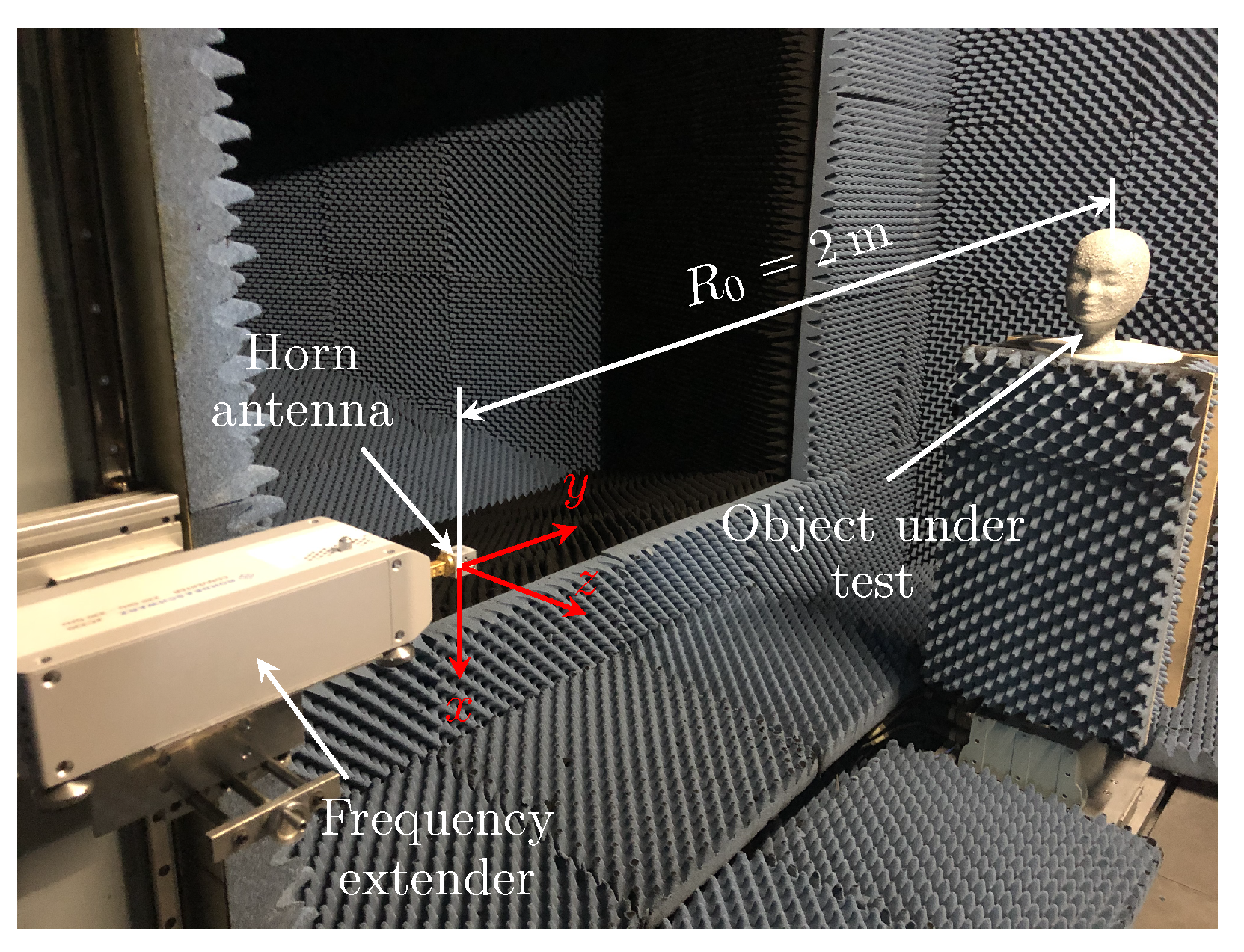
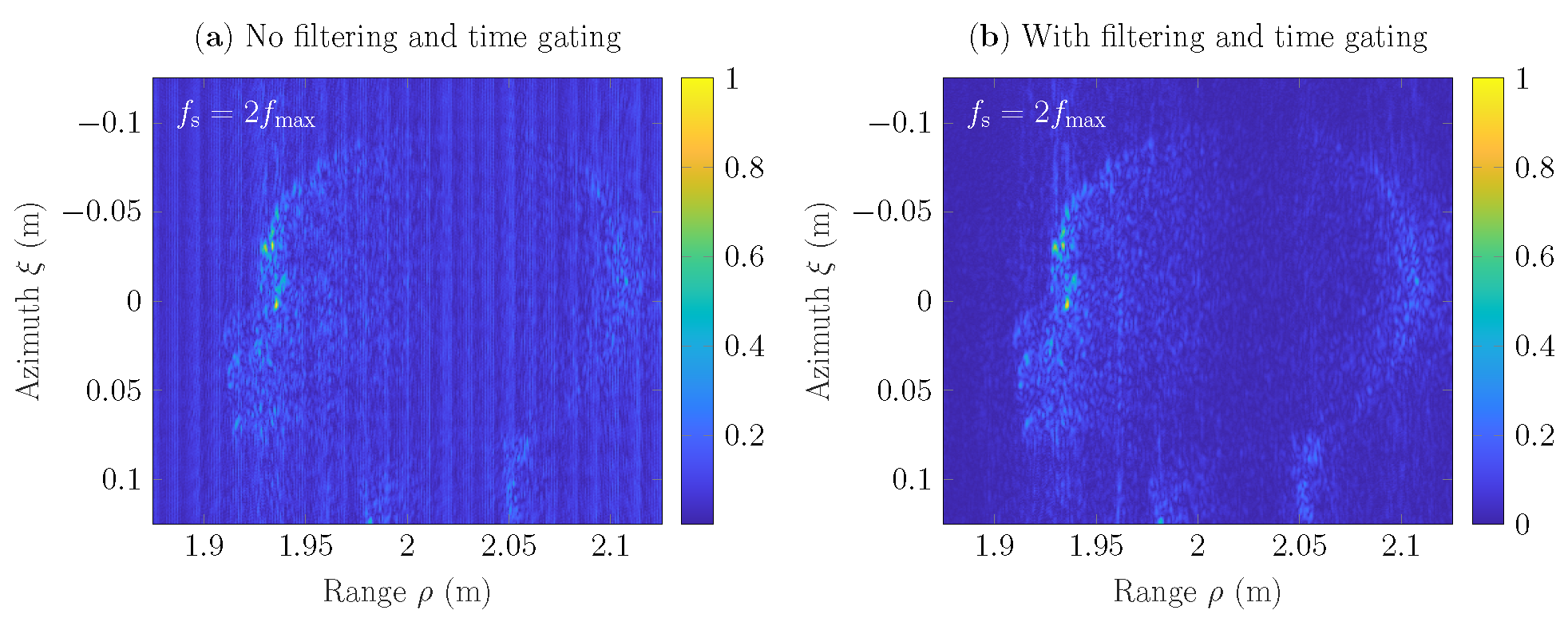
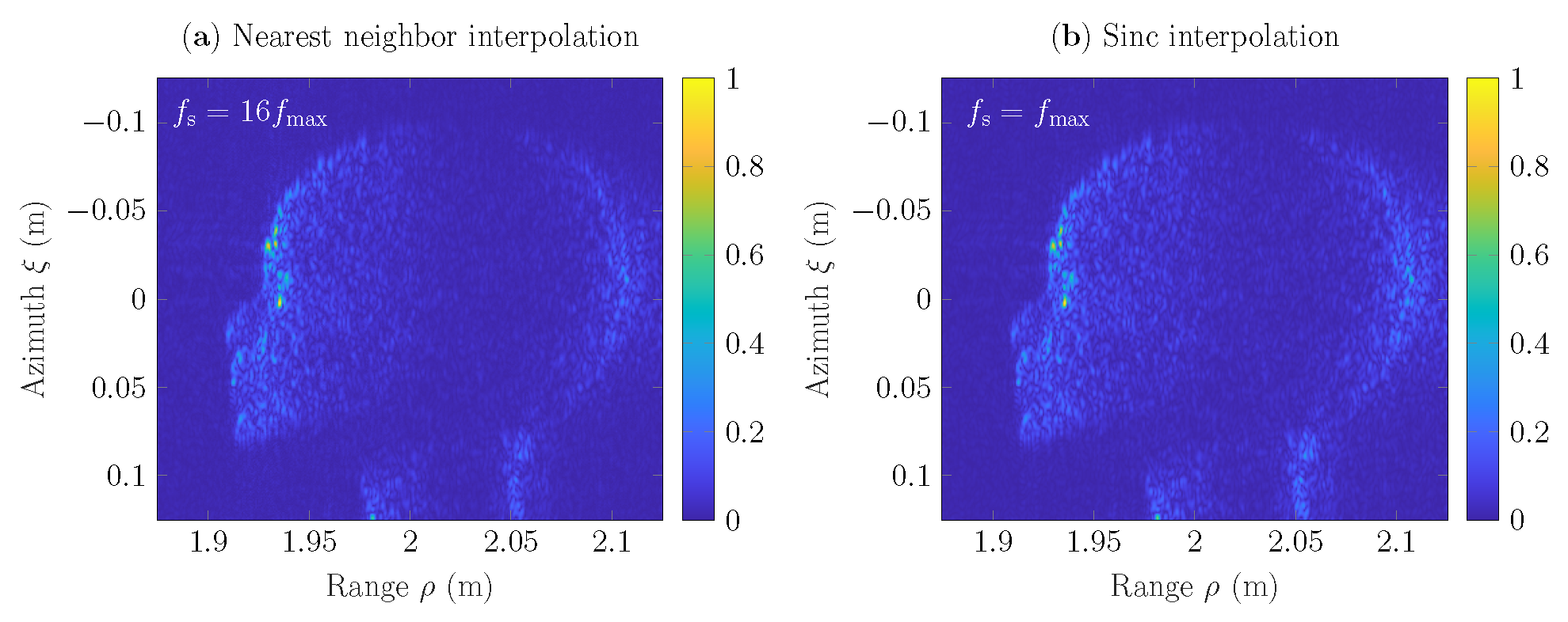
5. Experimentation
5.1. Measurement Setup
5.2. Results
6. Conclusions
Author Contributions
Funding
Institutional Review Board Statement
Informed Consent Statement
Data Availability Statement
Conflicts of Interest
Appendix A. Impulse Response Function
Appendix B. Peak-Sidelobe Ratio
References
- Carrara, W.; Carrara, W.; Goodman, R.; Majewski, R. Spotlight Synthetic Aperture Radar: Signal Processing Algorithms; Artech House Remote Sensing Library, Artech House: New York, NY, USA, 1995. [Google Scholar]
- Hellsten, H. Meter-Wave Synthetic Aperture Radar for Concealed Object Detection; Artech House: New York, NY, USA, 2017. [Google Scholar]
- Ottinger, M.; Kuenzer, C. Spaceborne L-Band Synthetic Aperture Radar Data for Geoscientific Analyses in Coastal Land Applications: A Review. Remote Sens. 2020, 12, 2228. [Google Scholar] [CrossRef]
- Vu, V.T.; Sjogren, T.K.; Pettersson, M.I.; Hellsten, H. An impulse response function for evaluation of UWB SAR imaging. IEEE Trans. Signal Process. 2010, 58, 3927–3932. [Google Scholar] [CrossRef] [Green Version]
- Vu, V.T.; Sjogren, T.K.; Pettersson, M.I. Fast time-domain algorithms for UWB bistatic SAR processing. IEEE Trans. Aerosp. Electron. Syst. 2013, 49, 1982–1994. [Google Scholar] [CrossRef] [Green Version]
- Hellsten, H.; Ulander, L.M.; Gustavsson, A.; Larsson, B. Development of VHF CARABAS II SAR. In Proceedings of the Radar Sensor Technology; International Society for Optics and Photonics: Bellingham, WA, USA, 1996; Volume 2747, pp. 48–60. [Google Scholar]
- Hellsten, H.; Ulander, L.M. Airborne array aperture UWB UHF radar-motivation and system considerations. IEEE Aerosp. Electron. Syst. Mag. 2000, 15, 35–45. [Google Scholar] [CrossRef]
- Caris, M.; Stanko, S.; Palm, S.; Sommer, R.; Wahlen, A.; Pohl, N. 300 GHz radar for high resolution SAR and ISAR applications. In Proceedings of the 2015 16th International Radar Symposium (IRS), Dresden, Germany, 24–26 June 2015; pp. 577–580. [Google Scholar]
- Zantah, Y.; Sheikh, F.; Abbas, A.A.; Alissa, M.; Kaiser, T. Channel measurements in lecture room environment at 300 GHz. In Proceedings of the 2019 Second International Workshop on Mobile Terahertz Systems (IWMTS), Bad Neuenahr, Germany, 1–3 July 2019; pp. 1–5. [Google Scholar]
- Batra, A.; Vu, V.T.; Zantah, Y.; Wiemeler, M.; Pettersson, M.I.; Goehringer, D.; Kaiser, T. Sub-mm Resolution Indoor THz Range and SAR Imaging of Concealed Object. In Proceedings of the 2020 IEEE MTT-S International Conference on Microwaves for Intelligent Mobility (ICMIM), Linz, Austria, 23 November 2020; pp. 1–4. [Google Scholar]
- Bryllert, T.; Cooper, K.B.; Dengler, R.J.; Llombart, N.; Chattopadhyay, G.; Schlecht, E.; Gill, J.; Lee, C.; Skalare, A.; Mehdi, I.; et al. A 600 GHz imaging radar for concealed objects detection. In Proceedings of the 2009 IEEE Radar Conference, Pasadena, CA, USA, 4–8 May 2009; pp. 1–3. [Google Scholar]
- Saqueb, S.; Nahar, N.; Sertel, K. Fast two-dimensional THz imaging using rail-based synthetic aperture radar (SAR) processing. Electron. Lett. 2020, 56, 988–990. [Google Scholar] [CrossRef]
- Batra, A.; Barowski, J.; Damyanov, D.; Wiemeler, M.; Rolfes, I.; Schultze, T.; Balzer, J.C.; Göhringer, D.; Kaiser, T. Short-Range SAR Imaging From GHz to THz Waves. IEEE J. Microwaves 2021, 1, 574–585. [Google Scholar] [CrossRef]
- Wang, H.; Zhang, Y.; Wang, B.; Sun, J. A novel helicopter-borne terahertz SAR imaging algorithm based on Keystone transform. In Proceedings of the 2014 12th International Conference on Signal Processing (ICSP), Hangzhou, China, 26–30 October 2014; pp. 1958–1962. [Google Scholar]
- Batra, A.; El-Absi, M.; Wiemeler, M.; Göhringer, D.; Kaiser, T. Indoor THz SAR Trajectory Deviations Effects and Compensation With Passive Sub-mm Localization System. IEEE Access 2020, 8, 177519–177533. [Google Scholar] [CrossRef]
- Andersson, L.E. On the determination of a function from spherical averages. SIAM J. Math. Anal. 1988, 19, 214–232. [Google Scholar] [CrossRef]
- Yegulalp, A.F. Fast backprojection algorithm for synthetic aperture radar. In Proceedings of the Proceedings of the 1999 IEEE Radar Conference. Radar into the Next Millennium (Cat. No. 99CH36249), Waltham, MA, USA, 22–22 April 1999; pp. 60–65. [Google Scholar]
- Ulander, L.M.H.; Hellsten, H.; Stenström, G. Synthetic-Aperture Radar Processing Using Fast Factorized Back-Projection. IEEE Trans. Aerosp. Electron. Syst. 2003, 39, 760–776. [Google Scholar] [CrossRef] [Green Version]
- Vu, V.T.; Pettersson, M.I. Derivation of bistatic SAR resolution equations based on backprojection. IEEE Geosci. Remote Sens. Lett. 2018, 15, 694–698. [Google Scholar] [CrossRef]
- Soumekh, M. Synthetic Aperture Radar Signal Processing with MATLAB Algorithms; John Wiley & Sons: New York, NY, USA, 1999. [Google Scholar]
- Hanssen, R.; Bamler, R. Evaluation of interpolation kernels for SAR interferometry. IEEE Trans. Geosci. Remote Sens. 1999, 37, 318–321. [Google Scholar] [CrossRef]
- Li, Z.; Bethel, J. Image coregistration in SAR interferometry. Int. Arch. Photogramm. Remote Sens. Spat. Inf. Sci. 2008, 37, 433–438. [Google Scholar]
- Capozzoli, A.; Curcio, C.; Liseno, A. Fast GPU-based interpolation for SAR backprojection. Prog. Electromagn. Res. 2013, 133, 259–283. [Google Scholar] [CrossRef] [Green Version]
- Ivanenko, Y.; Vu, V.T.; Pettersson, M.I. Interpolation Methods for SAR Backprojection at THz Frequencies. In Proceedings of the 2021 4th International Workshop on Mobile Terahertz Systems (IWMTS), Duisburg, Germany, 5–6 July 2021; pp. 1–5. [Google Scholar]
- Hellsten, H.; Andersson, L.E. An inverse method for the processing of synthetic aperture radar data. Inverse Probl. 1987, 3, 111–124. [Google Scholar] [CrossRef] [Green Version]
- Dahlquist, G.; Björck, Å. Numerical Methods; Prentice-Hall, Inc.: Englewood Cliffs, NJ, USA, 1974. [Google Scholar]
- De Boor, C. A Practical Guide to Splines, revised ed.; Applied Mathematical Sciences; Springer: New York, NY, USA, 2001; Volume 27. [Google Scholar]
- Proakis, J.G.; Manolakis, D.G. Digital Signal Processing, 4th ed.; Pearson Education, Inc.: London, UK, 2007. [Google Scholar]
- Bryant, G.H. Principles of Microwave Measurements; IET: London, UK, 1993; Volume 5. [Google Scholar]
- Vu, V.T.; Nehru, D.N.; Pettersson, M.I.; Sjögren, T.K. An experimental ground-based SAR system for studying SAR fundamentals. In Proceedings of the 2013 Asia-Pacific Conference on Synthetic Aperture Radar (APSAR), Tsukuba, Japan, 23–27 September 2013; pp. 424–427. [Google Scholar]
- Arfken, G.B.; Weber, H.J.; Harris, F.E. Mathematical Methods for Physicists, 7th ed.; Academic Press: New York, NY, USA, 2013. [Google Scholar]
- Vu, V.T.; Sjögren, T.K.; Pettersson, M.I.; Gustavsson, A. Definition on SAR image quality measurements for UWB SAR. In Proceedings of the Image and Signal Processing for Remote Sensing XIV, Cardiff, UK, 15–18 September 2008; Volume 7109, p. 71091A. [Google Scholar]


| Parameter | Value |
|---|---|
| The highest frequency processed, | |
| The lowest frequency processed, | |
| Number of aperture positions, | 345 |
| Aperture step, | |
| Integration angle, | ≈ |
| Reference range, |
|
Sampling Rate | |||
|---|---|---|---|
| Interpolation | |||
| Nearest neighbor | |||
| Linear | |||
| Cubic | |||
| Sinc | |||
| Analytical | |||
|
Sampling Rate | |||||
|---|---|---|---|---|---|
| Interpolation | |||||
| Nearest neighbor | |||||
| Linear | |||||
| Cubic | |||||
| Sinc | |||||
| Parameter | Value |
|---|---|
| The highest frequency processed, | |
| The lowest frequency processed, | |
| Number of aperture positions, | 344 |
| Number of frequency bins, | 3001 |
| Aperture step, | |
| Integration angle, | ≈ |
| Reference range, |
Publisher’s Note: MDPI stays neutral with regard to jurisdictional claims in published maps and institutional affiliations. |
© 2022 by the authors. Licensee MDPI, Basel, Switzerland. This article is an open access article distributed under the terms and conditions of the Creative Commons Attribution (CC BY) license (https://creativecommons.org/licenses/by/4.0/).
Share and Cite
Ivanenko, Y.; Vu, V.T.; Batra, A.; Kaiser, T.; Pettersson, M.I. Interpolation Methods with Phase Control for Backprojection of Complex-Valued SAR Data. Sensors 2022, 22, 4941. https://doi.org/10.3390/s22134941
Ivanenko Y, Vu VT, Batra A, Kaiser T, Pettersson MI. Interpolation Methods with Phase Control for Backprojection of Complex-Valued SAR Data. Sensors. 2022; 22(13):4941. https://doi.org/10.3390/s22134941
Chicago/Turabian StyleIvanenko, Yevhen, Viet T. Vu, Aman Batra, Thomas Kaiser, and Mats I. Pettersson. 2022. "Interpolation Methods with Phase Control for Backprojection of Complex-Valued SAR Data" Sensors 22, no. 13: 4941. https://doi.org/10.3390/s22134941
APA StyleIvanenko, Y., Vu, V. T., Batra, A., Kaiser, T., & Pettersson, M. I. (2022). Interpolation Methods with Phase Control for Backprojection of Complex-Valued SAR Data. Sensors, 22(13), 4941. https://doi.org/10.3390/s22134941