
A New Frequency Analysis Operator for Population Improvement in Genetic Algorithms to Solve the Job Shop Scheduling Problem †


Abstract
1. Introduction
2. Related Works
3. Formulation of the Job Shop Scheduling Problem
- Each job can be processed on a single machine at a time.
- Each machine can process only one job at a time.
- Operations are considered non-preemptive, i.e., they cannot be interrupted.
- Configuration times are included in the processing times and are independent of the sequencing decisions.
- is the set of jobs.
- is the set of machines.
- is an operation sequence that sets the priority order for processing the set of jobs in the set of machines.
- represents the time taken by the job to be processed by all machines in its script according to the operation sequence defined in O.
4. A New Genetic Improvement Operator Based on Frequency Analysis for GA Applied to JSSP
- A new strategy for defining genetic relevance in GAs chromosomes.
- A new genetic improvement operator that is versatile and can be used in GA variations.
- Improving the state of the art of JSSP benchmark results.
4.1. Genetic Representation
- (First) Job 2 must be processed by the first machine of its script.
- (Second) Job 1 must be processed by the first machine of its script.
- (Third) Job 2 must be processed by the second machine of its script.
- (Fourth) Job 2 must be processed by the third machine of its script.
- (Fifth) Job 1 must be processed by the second machine of its script.
- (Sixth) Job 1 must be processed by the third machine of its script.
4.2. Fitness Function
4.3. Proposed Genetic Improvement Based on Frequency Analysis Operator
| Algorithm 1 Defining the best individuals. | |
| Input: | Number of chromosomes in the population |
| Population | |
| F Fitness function | |
| Number of good individuals | |
| 1: | |
| 2: for to do | |
| 3: | |
| 4: | |
| 5: end for | |
| 6: ▹ The function ascending sorts the elements in a given set. In this case, is the index of the lowest fitness, is the index of the second-lowest fitness and so on, up to , which is the index of the highest fitness value. | |
| 7: ▹ We arrange individuals according to their fitness, from the best to the worst. | |
| 8: for to do | |
| 9: ▹ Let us define the best individuals. | |
| 10: end for | |
| Output: best individuals | |
| Algorithm 2 Calculating the genetic frequency of the best adapted individuals. | |
| Input: | best individuals |
| Dimension of JSSP instance | |
| 1: for to N do | |
| 2: ▹ Initializing the frequency vectors. In this case, is the null vector with coordinates. | |
| 3: end for | |
| 4: for to N do | |
| 5: for to do ▹ The value is the number of coordinates of chromosomes. | |
| 6: for to do | |
| 7: if then ▹ Is job i in the j-th coordinate of ? | |
| 8: ▹ If so, let us add 1 to the j-th coordinate of the frequency vector . | |
| 9: end if | |
| 10: end for | |
| 11: end for | |
| 12: end for | |
| Output: Frequency vectors | |
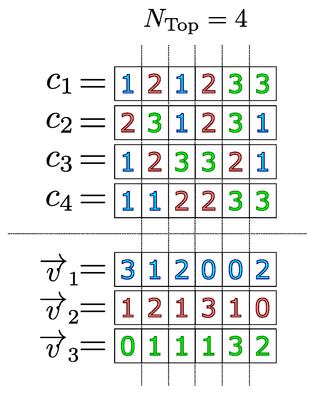
- Let be the representative individual and w a vector that designates a score for each of its coordinates, initially null. In the following items, the coordinates of and w are made.
- We define as being That is, is the index of the job that has the highest frequency in the first coordinate of the exemplary individuals. Therefore, the first coordinate of the representative individual is defined as . Mathematically,In addition, a score defined as the maximum frequency shown in the first coordinate of the best individuals is associated with the first coordinate of . That is,
- Assign the value 2 to j.
- We define as being that is, is the most frequent product index in the j coordinate in the individuals. However, in order to guarantee the feasibility of the representative individual, it is necessary to establish two more restrictions:
- 4.1
- If the product is not in M coordinates of , then it is defined as the j-th coordinate of the representative individual. That is,In this case, the respective score is associated with the j -th coordinate of the representative individual as the maximum possible value presented in the j-th coordinate of the best individuals. That is,
- 4.2
- Otherwise, to guarantee the feasibility of , the frequencies of the index job are disregarded, since it is already arranged in M coordinates of and, therefore, cannot occupy any more of its coordinates. To do so, we must cancel its respective frequency vector, that is,To make a new attempt, we must return to item 4.
- If then and we must return to item 4. Otherwise, the procedure is finished, and we have the representative individual pair and its respective genetic score .
| Algorithm 3 Calculating the representative individuals and their genetic relevance. | |
| Input: | Frequency vectors |
| Dimension of JSSP instance | |
| 1: ▹ Initialize the representative individual as being null. | |
| 2: ▹ Most frequent job in the first coordinate of the best individuals. | |
| 3: ▹ Number of times that the most frequent Job appears in the first coordinate of the best individuals. | |
| 4: ▹ Job occupies the first coordinate of the representative individual. | |
| 5: ▹ Concerning the next coordinates, we proceed similarly but guaranteeing feasibility. | |
| 6: while do | |
| 7: ▹ Let us calculate the most recurring job in the j-th coordinate of the frequency vectors. | |
| 8: ▹ To guarantee feasibility, each job must be in only M coordinates of the representative individual. | |
| 9: for to do | |
| 10: if then | |
| 11: | |
| 12: end if | |
| 13: end for | |
| 14: if then ▹ In case of feasibility, then we define the j-th coordinate of . | |
| 15: | |
| 16: | |
| 17: | |
| 18: else ▹ Otherwise, the next most recurring job in the j-th coordinate of the frequency vectors must be evaluated. | |
| 19: ▹ Since makes unfeasible, then we must disregard it for the next calculations. | |
| 20: end if | |
| 21: end while | |
| Output: | Representative individual |
| w Genetic relevance vector | |
4.3.1. Stage 2: Use of the Representative Individual in Genetic Improvement
| Algorithm 4 Population improvement using representative individual and genetic relevance. | |
| Input: | Representative individual |
| w Genetic relevance vector | |
| The worst individuals | |
| The JSSP dimension | |
| 1: ▹ Number of genes to be transferred. | |
| 2: for to do | |
| 3: ▹ coordinates that represent its most important genes. | |
| 4: | |
| 5: end for | |
| 6: for to do | |
| 7: for to do | |
| 8: ▹Transferring the best genes from to individuals in . | |
| 9: end for | |
| 10: end for | |
| 11: | |
| 12: for to do | |
| 13: ▹ Correcting infeasible solutions with Hamming projection. | |
| 14: | |
| 15: end for | |
| Output: Improved individuals | |
4.3.2. Generating New Individuals with the Lévy Flight Strategy
| Algorithm 5 Population improvement with diversity maintenance. | |
| Input: | Representative individual |
| w Genetic relevance vector | |
| The worst individuals | |
| The JSSP dimension | |
| F Fitness function | |
| 1: ▹ The set of individuals improved by the genetic improvement process is obtained through Algorithm 4. | |
| 2: for to do ▹ All improved individuals should be evaluated to ensure that the fitness has improved. | |
| 3: ▹ is the original individual. | |
| 4: ▹ is the improved individual. | |
| 5: if then ▹ In case there is no improvement, the individual in question must be replaced by a new individual generated from the random permutation, with this being defined by the Lévy distribution, of a feasible solution. | |
| 6: ▹ The individual from is removed. | |
| 7: ▹ The new individual is generated using the Lévy distribution. | |
| 8: ▹ The generated individual assumes its position in . | |
| 9: end if | |
| 10: end if | |
| Output: Improved individuals | |
4.4. Scheme of Use for Proposed Operators: Algorithm Structure
- Define the initial parameters and specifics of the chosen GA-like method.
- Execute the operators that make up the GA-like method. These being, for example, the operators of crossover, mutation, local search, creation of new population, etc.
- At the end of an iteration involving the traditional operators of the selected GA-like method, we make a sub-population with the worst individuals in the current population.
- At the same time, we select the best individuals in the population to compose the representative individual.
- Build the representative individual using the strategy described in Stage 1 of Section 4.3.
- Determine a relevance scale to the genes of the representative individual.
- Conduct the genetic improvement of the individuals using the most relevant genes of the representative individual.
- Replace in the current population of the method all individuals who obtained an improvement in the fitness value in the process of genetic improvement and return in the execution of the original operators of the considered GA-like method. Those who have not improved should be replaced by new individuals randomly generated according to Levy’s exponential distribution, following the procedure of Al-Obaidi and Hussein [55].
5. Implementation and Experimental Results
5.1. Experimental Environment
5.2. Results and Comparison with Other Algorithms
- There was no worsening of the results in any instance with the use of the GIFA operator;
- The GIFA-mXLSGA method had the smallest relative error;
- The GIFA operator made mXLSGA able to find the best known solution in instance LA 22;
- GIFA operator improved mXLSGA results in 7 LA instances;
- The GIFA operator made mXLSGA able to find the best known solution in instance ORB06 and improved the solution obtained in ORB05,
- The GIFA operator reduced the average error of mXLSGA by 53% in ABZ instances.
6. Conclusions
Author Contributions
Funding
Institutional Review Board Statement
Informed Consent Statement
Conflicts of Interest
References
- Pardalos, P.M.; Du, D.Z.; Graham, R.L. Handbook of Combinatorial Optimization; Springer: Berlin/Heidelberg, Germany, 2013. [Google Scholar]
- Sbihi, A.; Eglese, R.W. Combinatorial optimization and green logistics. Ann. Oper. Res. 2010, 175, 159–175. [Google Scholar] [CrossRef]
- James, J.; Yu, W.; Gu, J. Online vehicle routing with neural combinatorial optimization and deep reinforcement learning. IEEE Trans. Intell. Transp. Syst. 2019, 20, 3806–3817. [Google Scholar]
- Matyukhin, V.; Shabunin, A.; Kuznetsov, N.; Takmazian, A. Rail transport control by combinatorial optimization approach. In Proceedings of the 2017 IEEE 11th International Conference on Application of Information and Communication Technologies (AICT), Moscow, Russia, 20–22 September 2017; pp. 1–4. [Google Scholar]
- Ehrgott, M.; Gandibleux, X. Multiobjective combinatorial optimization—Theory, methodology, and applications. In Multiple Criteria Optimization: State of the Art Annotated Bibliographic Surveys; Springer: Boston, MA, USA, 2003; pp. 369–444. [Google Scholar]
- Parente, M.; Figueira, G.; Amorim, P.; Marques, A. Production scheduling in the context of Industry 4.0: Review and trends. Int. J. Prod. Res. 2020, 58, 5401–5431. [Google Scholar] [CrossRef]
- Groover, M.P. Fundamentals of Modern Manufacturing: Materials Processes, and Systems; John Wiley & Sons: Hoboken, NJ, USA, 2007. [Google Scholar]
- Hart, E.; Ross, P.; Corne, D. Evolutionary scheduling: A review. Genet. Program. Evolvable Mach. 2005, 6, 191–220. [Google Scholar] [CrossRef]
- Xhafa, F.; Abraham, A. Metaheuristics for Scheduling in Industrial and Manufacturing Applications; Springer: Berlin/Heidelberg, Germany, 2008; Volume 128. [Google Scholar]
- Wu, Z.; Sun, S.; Yu, S. Optimizing makespan and stability risks in job shop scheduling. Comput. Oper. Res. 2020, 122, 104963. [Google Scholar] [CrossRef]
- Wang, L.; Cai, J.C.; Li, M. An adaptive multi-population genetic algorithm for job-shop scheduling problem. Adv. Manuf. 2016, 4, 142–149. [Google Scholar] [CrossRef]
- Mhasawade, S.; Bewoor, L. A survey of hybrid metaheuristics to minimize makespan of job shop scheduling problem. In Proceedings of the 2017 International Conference on Energy, Communication, Data Analytics and Soft Computing (ICECDS), Chennai, India, 1–2 August 2017; pp. 1957–1960. [Google Scholar]
- Viana, M.S.; Morandin Junior, O.; Contreras, R.C. A Modified Genetic Algorithm with Local Search Strategies and Multi-Crossover Operator for Job Shop Scheduling Problem. Sensors 2020, 20, 5440. [Google Scholar] [CrossRef]
- Viana, M.S.; Morandin Junior, O.; Contreras, R.C. An Improved Local Search Genetic Algorithm with Multi-Crossover for Job Shop Scheduling Problem. In Proceedings of the International Conference on Artificial Intelligence and Soft Computing, Zakopane, Poland, 12–14 October 2020; Springer: Zakopane, Poland, 2020; pp. 464–479. [Google Scholar]
- Viana, M.S.; Morandin Junior, O.; Contreras, R.C. Transgenic Genetic Algorithm to Minimize the Makespan in the Job Shop Scheduling Problem. In Proceedings of the 12th International Conference on Agents and Artificial Intelligence—Volume 2: ICAART. INSTICC, Valletta, Malta, February 22–24; SciTePress: Setubal, Portugal, 2020; pp. 463–474. [Google Scholar] [CrossRef]
- Lu, Y.; Huang, Z.; Cao, L. Hybrid immune genetic algorithm with neighborhood search operator for the Job Shop Scheduling Problem. IOP Conf. Ser. Earth Environ. Sci. 2020, Volume 474, 052093. [Google Scholar]
- Milovsevic, M.; Lukic, D.; Durdev, M.; Vukman, J.; Antic, A. Genetic algorithms in integrated process planning and scheduling—A state of the art review. Proc. Manuf. Syst. 2016, 11, 83–88. [Google Scholar]
- Çaliş, B.; Bulkan, S. A research survey: Review of AI solution strategies of job shop scheduling problem. J. Intell. Manuf. 2015, 26, 961–973. [Google Scholar] [CrossRef]
- Demirkol, E.; Mehta, S.; Uzsoy, R. Benchmarks for shop scheduling problems. Eur. J. Oper. Res. 1998, 109, 137–141. [Google Scholar] [CrossRef]
- Asadzadeh, L. A local search genetic algorithm for the job shop scheduling problem with intelligent agents. Comput. Ind. Eng. 2015, 85, 376–383. [Google Scholar] [CrossRef]
- Contreras, R.C.; Morandin Junior, O.; Viana, M.S. A New Local Search Adaptive Genetic Algorithm for the Pseudo-Coloring Problem. In Advances in Swarm Intelligence; Springer: Cham, Switzerland, 2020; pp. 349–361. [Google Scholar]
- Viana, M.S.; Morandin Junior, O.; Contreras, R.C. An Improved Local Search Genetic Algorithm with a New Mapped Adaptive Operator Applied to Pseudo-Coloring Problem. Symmetry 2020, 12, 1684. [Google Scholar] [CrossRef]
- Zang, W.; Ren, L.; Zhang, W.; Liu, X. A cloud model based DNA genetic algorithm for numerical optimization problems. Future Gener. Comput. Syst. 2018, 81, 465–477. [Google Scholar] [CrossRef]
- Li, X.; Gao, L. An effective hybrid genetic algorithm and tabu search for flexible job shop scheduling problem. Int. J. Prod. Econ. 2016, 174, 93–110. [Google Scholar] [CrossRef]
- Sastry, K.; Goldberg, D.; Kendall, G. Genetic algorithms. In Search Methodologies; Springer: Boston, MA, USA, 2005; pp. 97–125. [Google Scholar]
- do Amaral, L.R.; Hruschka, E.R. Transgenic, an operator for evolutionary algorithms. In Proceedings of the 2011 IEEE Congress of Evolutionary Computation (CEC), New Orleans, LA, USA, 5–8 June 2011; pp. 1308–1314. [Google Scholar]
- do Amaral, L.R.; Hruschka, E.R., Jr. Transgenic: An evolutionary algorithm operator. Neurocomputing 2014, 127, 104–113. [Google Scholar] [CrossRef]
- Viana, M.S.; Contreras, R.C.; Junior, O.M. A New Genetic Improvement Operator Based on Frequency Analysis for Genetic Algorithms Applied to Job Shop Scheduling Problem. In Proceedings of the International Conference on Artificial Intelligence and Soft Computing, Zakopane, Poland, 20–24 June 2021; Springer: Zakopane, Poland, 2021; pp. 434–450. [Google Scholar]
- Ombuki, B.M.; Ventresca, M. Local search genetic algorithms for the job shop scheduling problem. Appl. Intell. 2004, 21, 99–109. [Google Scholar] [CrossRef]
- Watanabe, M.; Ida, K.; Gen, M. A genetic algorithm with modified crossover operator and search area adaptation for the job-shop scheduling problem. Comput. Ind. Eng. 2005, 48, 743–752. [Google Scholar] [CrossRef]
- Jorapur, V.S.; Puranik, V.S.; Deshpande, A.S.; Sharma, M. A promising initial population based genetic algorithm for job shop scheduling problem. J. Softw. Eng. Appl. 2016, 9, 208. [Google Scholar] [CrossRef]
- Kurdi, M. An effective genetic algorithm with a critical-path-guided Giffler and Thompson crossover operator for job shop scheduling problem. Int. J. Intell. Syst. Appl. Eng. 2019, 7, 13–18. [Google Scholar] [CrossRef][Green Version]
- Liang, X.; Du, Z. Genetic Algorithm with Simulated Annealing for Resolving Job Shop Scheduling Problem. In Proceedings of the 2020 IEEE 8th International Conference on Computer Science and Network Technology (ICCSNT), Dalian, China, 20–22 November 2020; pp. 64–68. [Google Scholar] [CrossRef]
- Anil Kumar, K.R.; Das, E.R. Genetic Algorithm and Particle Swarm Optimization in Minimizing MakeSpan Time in Job Shop Scheduling. In Proceedings of ICDMC 2019; Yang, L.J., Haq, A.N., Nagarajan, L., Eds.; Springer: Singapore, 2020; pp. 421–432. [Google Scholar]
- Zhang, J.; Cong, J. Research on job shop scheduling based on ACM-GA algorithm. In Proceedings of the 2021 IEEE 5th Advanced Information Technology, Electronic and Automation Control Conference (IAEAC), Chongqing, China, 12–14 March 2021; Volume 5, pp. 490–495. [Google Scholar] [CrossRef]
- Wang, B.; Wang, X.; Lan, F.; Pan, Q. A hybrid local-search algorithm for robust job-shop scheduling under scenarios. Appl. Soft Comput. 2018, 62, 259–271. [Google Scholar] [CrossRef]
- Frausto-Solis, J.; Hernández-Ramírez, L.; Castilla-Valdez, G.; González-Barbosa, J.J.; Sánchez-Hernández, J.P. Chaotic Multi-Objective Simulated Annealing and Threshold Accepting for Job Shop Scheduling Problem. Math. Comput. Appl. 2021, 26, 8. [Google Scholar] [CrossRef]
- Zhou, G.; Zhou, Y.; Zhao, R. Hybrid social spider optimization algorithm with differential mutation operator for the job-shop scheduling problem. J. Ind. Manag. Optim. 2021, 17, 533–548. [Google Scholar] [CrossRef]
- Liu, C. An improved Harris hawks optimizer for job-shop scheduling problem. J. Supercomput. 2021, 77, 14090–14129. [Google Scholar] [CrossRef]
- Jiang, T. A Hybrid Grey Wolf Optimization for Job Shop Scheduling Problem. Int. J. Comput. Intell. Appl. 2018, 17, 1850016. [Google Scholar] [CrossRef]
- Dao, T.K.; Pan, T.S.; Pan, J.S. Parallel bat algorithm for optimizing makespan in job shop scheduling problems. J. Intell. Manuf. 2018, 29, 451–462. [Google Scholar] [CrossRef]
- Semlali, S.C.B.; Riffi, M.E.; Chebihi, F. Memetic chicken swarm algorithm for job shop scheduling problem. Int. J. Electr. Comput. Eng. 2019, 9, 2075. [Google Scholar] [CrossRef]
- Hamzadayı, A.; Baykasoğlu, A.; Akpınar, Ş. Solving combinatorial optimization problems with single seekers society algorithm. Knowl.-Based Syst. 2020, 201, 106036. [Google Scholar] [CrossRef]
- Yu, H.; Gao, Y.; Wang, L.; Meng, J. A Hybrid Particle Swarm Optimization Algorithm Enhanced with Nonlinear Inertial Weight and Gaussian Mutation for Job Shop Scheduling Problems. Mathematics 2020, 8, 1355. [Google Scholar] [CrossRef]
- Fisher, C.; Thompson, G. Probabilistic learning combinations of local job-shop scheduling rules. In Industrial Scheduling; Prentice-Hall: Englewood Cliffs, NJ, USA, 1963; pp. 225–251. [Google Scholar]
- Lawrence, S. Resouce Constrained Project Scheduling: An Experimental Investigation of Heuristic Scheduling Techniques (Supplement); Graduate School of Industrial Administration, Carnegie-Mellon University: Pittsburgh, PA, USA, 1984. [Google Scholar]
- Croes, G.A. A method for solving traveling-salesman problems. Oper. Res. 1958, 6, 791–812. [Google Scholar] [CrossRef]
- Meng, X.; Liu, Y.; Gao, X.; Zhang, H. A new bio-inspired algorithm: Chicken swarm optimization. In Proceedings of the International Conference in Swarm Intelligence, Hefei, China, 17–20 October 2014; Springer: Cham, Switzerland, 2014; pp. 86–94. [Google Scholar]
- Alkhateeb, F.; Abed-alguni, B.H.; Al-rousan, M.H. Discrete hybrid cuckoo search and simulated annealing algorithm for solving the job shop scheduling problem. J. Supercomput. 2022, 78, 4799–4826. [Google Scholar] [CrossRef]
- Xiong, H.; Shi, S.; Ren, D.; Hu, J. A survey of job shop scheduling problem: The types and models. Comput. Oper. Res. 2022, 142, 105731. [Google Scholar] [CrossRef]
- Bierwirth, C.; Mattfeld, D.C.; Kopfer, H. On permutation representations for scheduling problems. In Proceedings of the International Conference on Parallel Problem Solving from Nature, Berlin, Germany, 22 – 26 September; Springer: Berlin/Heidelberg, Germany, 1996; pp. 310–318. [Google Scholar]
- Wegner, P. A Technique for Counting Ones in a Binary Computer. Commun. ACM 1960, 3, 322. [Google Scholar] [CrossRef]
- Yang, X.S.; Deb, S. Multiobjective cuckoo search for design optimization. Comput. Oper. Res. 2013, 40, 1616–1624. [Google Scholar] [CrossRef]
- Yang, X.S. Engineering Optimization: An Introduction with Metaheuristic Applications; John Wiley & Sons: Hoboken, NJ, USA, 2010. [Google Scholar]
- Al-Obaidi, A.T.S.; Hussein, S.A. Two improved cuckoo search algorithms for solving the flexible job-shop scheduling problem. Int. J. Perceptive Cogn. Comput. 2016, 2. [Google Scholar] [CrossRef]
- Applegate, D.; Cook, W. A computational study of the job-shop scheduling problem. ORSA J. Comput. 1991, 3, 149–156. [Google Scholar] [CrossRef]
- Adams, J.; Balas, E.; Zawack, D. The shifting bottleneck procedure for job shop scheduling. Manag. Sci. 1988, 34, 391–401. [Google Scholar] [CrossRef]
- Wang, F.; Tian, Y.; Wang, X. A Discrete Wolf Pack Algorithm for Job Shop Scheduling Problem. In Proceedings of the 2019 5th International Conference on Control, Automation and Robotics (ICCAR), Beijing, China, 19–22 April 2019; pp. 581–585. [Google Scholar]
- Jiang, T.; Zhang, C. Application of grey wolf optimization for solving combinatorial problems: Job shop and flexible job shop scheduling cases. IEEE Access 2018, 6, 26231–26240. [Google Scholar] [CrossRef]
- Kurdi, M. An effective new island model genetic algorithm for job shop scheduling problem. Comput. Oper. Res. 2016, 67, 132–142. [Google Scholar] [CrossRef]
- Asadzadeh, L.; Zamanifar, K. An agent-based parallel approach for the job shop scheduling problem with genetic algorithms. Math. Comput. Model. 2010, 52, 1957–1965. [Google Scholar] [CrossRef]
- Xie, J.; Gao, L.; Peng, K.; Li, X.; Li, H. Review on flexible job shop scheduling. IET Collab. Intell. Manuf. 2019, 1, 67–77. [Google Scholar] [CrossRef]


| Instance | Method | Best | Worst | Mean | SD | Number of Optima | Iteration of the Optimum | Time (s) |
|---|---|---|---|---|---|---|---|---|
| FT06 | GA | 55 | 57 | 55.45 | 0.85 | 27 | 52 | 2.4 |
| GIFA-GA | 55 | 56 | 55.14 | 0.35 | 30 | 38 | 2.63 | |
| GSA | 55 | 55 | 55 | 0 | 35 | 8 | 39.78 | |
| GIFA-GSA | 55 | 55 | 55 | 0 | 35 | 8 | 40.02 | |
| LSGA | 55 | 59 | 57.68 | 1.43 | 6 | 27 | 7.95 | |
| GIFA-LSGA | 55 | 56 | 55.83 | 0.38 | 6 | 20 | 8.17 | |
| aLSGA | 55 | 55 | 55 | 0 | 35 | 11 | 11.51 | |
| GIFA-aLSGA | 55 | 55 | 55 | 0 | 35 | 6 | 13.01 | |
| mXLSGA | 55 | 55 | 55 | 0 | 35 | 5 | 22.11 | |
| GIFA-mXLSGA | 55 | 55 | 55 | 0 | 35 | 5 | 22.37 | |
| LA01 | GA | 666 | 712 | 679.02 | 9.98 | 6 | 76 | 2.65 |
| GIFA-GA | 666 | 678 | 669.37 | 5.17 | 15 | 26 | 2.94 | |
| GSA | 666 | 715 | 677.8 | 13.61 | 13 | 10 | 51.79 | |
| GIFA-GSA | 666 | 687 | 672.34 | 7.43 | 17 | 10 | 51.96 | |
| LSGA | 666 | 726 | 697 | 16.65 | 1 | 61 | 12.15 | |
| GIFA-LSGA | 666 | 707 | 688.67 | 15.59 | 8 | 23 | 12.42 | |
| aLSGA | 666 | 666 | 666 | 0 | 35 | 11 | 20.07 | |
| GIFA-aLSGA | 666 | 666 | 666 | 0 | 35 | 6 | 20.29 | |
| mXLSGA | 666 | 666 | 666 | 0 | 35 | 5 | 38.06 | |
| GIFA-mXLSGA | 666 | 666 | 666 | 0 | 35 | 4 | 38.34 | |
| LA06 | GA | 926 | 938 | 927.4 | 2.87 | 24 | 79 | 3.34 |
| GIFA-GA | 926 | 936 | 926.86 | 2.26 | 30 | 54 | 3.57 | |
| GSA | 926 | 935 | 926.31 | 1.54 | 33 | 7 | 67.31 | |
| GIFA-GSA | 926 | 926 | 926 | 0 | 35 | 7 | 67.56 | |
| LSGA | 926 | 970 | 935.8 | 13.15 | 17 | 55 | 19.87 | |
| GIFA-LSGA | 926 | 952 | 932.28 | 9.08 | 20 | 41 | 20.13 | |
| aLSGA | 926 | 926 | 926 | 0 | 35 | 3 | 38.07 | |
| GIFA-aLSGA | 926 | 926 | 926 | 0 | 35 | 3 | 38.31 | |
| mXLSGA | 926 | 926 | 926 | 0 | 35 | 2 | 71.98 | |
| GIFA-mXLSGA | 926 | 926 | 926 | 0 | 35 | 2 | 72.21 | |
| LA11 | GA | 1222 | 1256 | 1235.97 | 10.81 | 5 | 58 | 3.97 |
| GIFA-GA | 1222 | 1253 | 1233.48 | 9.52 | 6 | 51 | 4.18 | |
| GSA | 1222 | 1276 | 1232.14 | 14.94 | 20 | 19 | 81.59 | |
| GIFA-GSA | 1222 | 1263 | 1231.24 | 13.56 | 26 | 15 | 81.7 | |
| LSGA | 1222 | 1299 | 1251.6 | 19.62 | 2 | 32 | 31.33 | |
| GIFA-LSGA | 1222 | 1278 | 1250.17 | 11.09 | 4 | 26 | 31.59 | |
| aLSGA | 1222 | 1222 | 1222 | 0 | 35 | 5 | 60.82 | |
| GIFA-aLSGA | 1222 | 1222 | 1222 | 0 | 35 | 4 | 61.03 | |
| mXLSGA | 1222 | 1222 | 1222 | 0 | 35 | 3 | 116.57 | |
| GIFA-mXLSGA | 1222 | 1222 | 1222 | 0 | 35 | 3 | 116.84 | |
| LA16 | GA | 982 | 1100 | 1045.6 | 26.4 | 0 | - | 2.89 |
| GIFA-GA | 982 | 1061 | 1022.89 | 20.51 | 0 | - | 3.12 | |
| GSA | 994 | 1110 | 1046.77 | 26.37 | 0 | - | 55.31 | |
| GIFA-GSA | 994 | 1021 | 1017.38 | 15.49 | 0 | - | 55.63 | |
| LSGA | 1016 | 1148 | 1084.25 | 32.27 | 0 | - | 20.62 | |
| GIFA-LSGA | 1016 | 1077 | 1037.11 | 26.62 | 0 | - | 20.83 | |
| aLSGA | 959 | 985 | 980.51 | 4.48 | 0 | - | 38.75 | |
| GIFA-aLSGA | 956 | 982 | 975.12 | 2.36 | 0 | - | 38.98 | |
| mXLSGA | 945 | 982 | 972.25 | 13.3 | 2 | 96 | 66.25 | |
| GIFA-mXLSGA | 945 | 979 | 959.93 | 6.37 | 7 | 49 | 66.51 | |
| LA23 | GA | 1189 | 1336 | 1271.71 | 34.44 | 0 | - | 3.78 |
| GIFA-GA | 1151 | 1324 | 1269.51 | 30.95 | 0 | - | 4 | |
| GSA | 1148 | 1347 | 1214.08 | 43.85 | 0 | - | 73.19 | |
| GIFA-GSA | 1121 | 1339 | 1191.25 | 30.27 | 0 | - | 73.42 | |
| LSGA | 1214 | 1419 | 1295.34 | 43.7 | 0 | - | 38.39 | |
| GIFA-LSGA | 1115 | 1369 | 1278.36 | 34.79 | 0 | - | 38.63 | |
| aLSGA | 1035 | 1115 | 1078 | 16.34 | 0 | - | 75.62 | |
| GIFA-aLSGA | 1032 | 1098 | 1067.58 | 15.06 | 2 | 75 | 75.79 | |
| mXLSGA | 1032 | 1093 | 1060.45 | 17.96 | 1 | 51 | 123.64 | |
| GIFA-mXLSGA | 1032 | 1093 | 1039.8 | 16.54 | 2 | 34 | 123.87 | |
| LA26 | GA | 1525 | 1699 | 1619.51 | 39.5 | 0 | - | 4.44 |
| GIFA-GA | 1485 | 1667 | 1614.11 | 32.59 | 0 | - | 4.65 | |
| GSA | 1433 | 1586 | 1512.22 | 36.47 | 0 | - | 91.67 | |
| GIFA-GSA | 1420 | 1523 | 1503.73 | 17.99 | 0 | - | 91.94 | |
| LSGA | 1517 | 1665 | 1597.94 | 36.67 | 0 | - | 60.84 | |
| GIFA-LSGA | 1492 | 1537 | 1534.11 | 28.74 | 0 | - | 61.07 | |
| aLSGA | 1302 | 1384 | 1343.28 | 19.69 | 0 | - | 124.93 | |
| GIFA-aLSGA | 1273 | 1382 | 1332.68 | 13.28 | 0 | - | 125.12 | |
| mXLSGA | 1218 | 1371 | 1300.85 | 41.88 | 6 | 85 | 203.95 | |
| GIFA-mXLSGA | 1218 | 1371 | 1258.51 | 32.32 | 11 | 67 | 204.3 | |
| LA31 | GA | 2120 | 2326 | 2223.14 | 48.45 | 0 | - | 6.23 |
| GIFA-GA | 2111 | 2322 | 2197.31 | 45.19 | 0 | - | 6.51 | |
| GSA | 1943 | 2142 | 2050.17 | 63.09 | 0 | - | 130.65 | |
| GIFA-GSA | 1919 | 2101 | 1964.2 | 56.94 | 0 | - | 130.89 | |
| LSGA | 2005 | 2336 | 2177 | 66.29 | 0 | - | 123.23 | |
| GIFA-LSGA | 1986 | 2301 | 2119.88 | 62.49 | 0 | - | 123.57 | |
| aLSGA | 1808 | 1897 | 1843.51 | 21.17 | 0 | - | 258.53 | |
| GIFA-aLSGA | 1784 | 1861 | 1841.25 | 19.13 | 2 | 80 | 258.81 | |
| mXLSGA | 1784 | 1845 | 1807.71 | 19.2 | 5 | 80 | 424.56 | |
| GIFA-mXLSGA | 1784 | 1845 | 1805.98 | 18.96 | 7 | 71 | 424.77 |
| Instance | Size | BKS | GIFA-mXLSGA | mXLSGA | NGPSO | SSS | GA-CPG-GT | GWO | IPB-GA | aLSGA | ||||||||
|---|---|---|---|---|---|---|---|---|---|---|---|---|---|---|---|---|---|---|
| Best | Best | Best | Best | Best | Best | Best | Best | |||||||||||
| FT06 | 55 | 55 | 0.00 | 55 | 0.00 | 55 | 0.00 | 55 | 0.00 | 55 | 0.00 | 55 | 0.00 | 55 | 0.00 | 55 | 0.00 | |
| FT10 | 930 | 930 | 0.00 | 930 | 0.00 | 930 | 0.00 | 936 | 0.64 | 935 | 0.53 | 940 | 1.07 | 960 | 3.22 | 930 | 0.00 | |
| FT20 | 1165 | 1165 | 0.00 | 1165 | 0.00 | 1210 | 3.86 | 1165 | 0.00 | 1180 | 1.28 | 1178 | 1.11 | 1192 | 2.31 | 1165 | 0.00 | |
| MErr | 0.00 | 0.00 | 1.28 | 0.21 | 0.60 | 0.73 | 1.84 | 0.00 | ||||||||||
| Instance | Size | BKS | GIFA-mXLSGA | mXLSGA | NGPSO | SSS | GA-CPG-GT | DWPA | GWO | IPB-GA | aLSGA | |||||||||
|---|---|---|---|---|---|---|---|---|---|---|---|---|---|---|---|---|---|---|---|---|
| Best | Best | Best | Best | Best | Best | Best | Best | Best | ||||||||||||
| LA01 | 666 | 666 | 0.00 | 666 | 0.00 | 666 | 0.00 | 666 | 0.00 | 666 | 0.00 | 666 | 0.00 | 666 | 0.00 | 666 | 0.00 | 666 | 0.00 | |
| LA02 | 655 | 655 | 0.00 | 655 | 0.00 | 655 | 0.00 | 655 | 0.00 | 655 | 0.00 | 655 | 0.00 | 655 | 0.00 | 655 | 0.00 | 655 | 0.00 | |
| LA03 | 597 | 597 | 0.00 | 597 | 0.00 | 597 | 0.00 | 597 | 0.00 | 597 | 0.00 | 614 | 2.84 | 597 | 0.00 | 599 | 0.33 | 606 | 1.50 | |
| LA04 | 590 | 590 | 0.00 | 590 | 0.00 | 590 | 0.00 | 590 | 0.00 | 590 | 0.00 | 598 | 1.35 | 590 | 0.00 | 590 | 0.00 | 593 | 0.50 | |
| LA05 | 593 | 593 | 0.00 | 593 | 0.00 | 593 | 0.00 | 593 | 0.00 | 593 | 0.00 | 593 | 0.00 | 593 | 0.00 | 593 | 0.00 | 593 | 0.00 | |
| LA06 | 926 | 926 | 0.00 | 926 | 0.00 | 926 | 0.00 | 926 | 0.00 | 926 | 0.00 | 926 | 0.00 | 926 | 0.00 | 926 | 0.00 | 926 | 0.00 | |
| LA07 | 890 | 890 | 0.00 | 890 | 0.00 | 890 | 0.00 | 890 | 0.00 | 890 | 0.00 | 890 | 0.00 | 890 | 0.00 | 890 | 0.00 | 890 | 0.00 | |
| LA08 | 863 | 863 | 0.00 | 863 | 0.00 | 863 | 0.00 | 863 | 0.00 | 863 | 0.00 | 863 | 0.00 | 863 | 0.00 | 863 | 0.00 | 863 | 0.00 | |
| LA09 | 951 | 951 | 0.00 | 951 | 0.00 | 951 | 0.00 | 951 | 0.00 | 951 | 0.00 | 951 | 0.00 | 951 | 0.00 | 951 | 0.00 | 951 | 0.00 | |
| LA10 | 958 | 958 | 0.00 | 958 | 0.00 | 958 | 0.00 | 958 | 0.00 | 958 | 0.00 | 958 | 0.00 | 958 | 0.00 | 958 | 0.00 | 958 | 0.00 | |
| LA11 | 1222 | 1222 | 0.00 | 1222 | 0.00 | 1222 | 0.00 | 1222 | 0.00 | 1222 | 0.00 | 1222 | 0.00 | 1222 | 0.00 | 1222 | 0.00 | 1222 | 0.00 | |
| LA12 | 1039 | 1039 | 0.00 | 1039 | 0.00 | 1039 | 0.00 | - | - | 1039 | 0.00 | 1039 | 0.00 | 1039 | 0.00 | 1039 | 0.00 | 1039 | 0.00 | |
| LA13 | 1150 | 1150 | 0.00 | 1150 | 0.00 | 1150 | 0.00 | - | - | 1150 | 0.00 | 1150 | 0.00 | 1150 | 0.00 | 1150 | 0.00 | 1150 | 0.00 | |
| LA14 | 1292 | 1292 | 0.00 | 1292 | 0.00 | 1292 | 0.00 | - | - | 1292 | 0.00 | 1292 | 0.00 | 1292 | 0.00 | 1292 | 0.00 | 1292 | 0.00 | |
| LA15 | 1207 | 1207 | 0.00 | 1207 | 0.00 | 1207 | 0.00 | - | - | 1207 | 0.00 | 1273 | 5.46 | 1207 | 0.00 | 1207 | 0.00 | 1207 | 0.00 | |
| LA16 | 945 | 945 | 0.00 | 945 | 0.00 | 945 | 0.00 | 947 | 0.21 | 946 | 0.10 | 993 | 5.07 | 956 | 1.16 | 946 | 0.10 | 946 | 0.10 | |
| LA17 | 784 | 784 | 0.00 | 784 | 0.00 | 794 | 1.27 | - | - | 784 | 0.00 | 793 | 1.14 | 790 | 0.76 | 784 | 0.00 | 784 | 0.00 | |
| LA18 | 848 | 848 | 0.00 | 848 | 0.00 | 848 | 0.00 | - | - | 848 | 0.00 | 861 | 1.53 | 859 | 1.29 | 853 | 0.58 | 848 | 0.00 | |
| LA19 | 842 | 842 | 0.00 | 842 | 0.00 | 842 | 0.00 | - | - | 842 | 0.00 | 888 | 5.46 | 845 | 0.35 | 866 | 2.85 | 852 | 1.18 | |
| LA20 | 902 | 902 | 0.00 | 902 | 0.00 | 908 | 0.66 | - | - | 907 | 0.55 | 934 | 3.54 | 937 | 3.88 | 913 | 1.21 | 907 | 0.55 | |
| LA21 | 1046 | 1052 | 0.57 | 1059 | 1.24 | 1183 | 13.09 | 1076 | 2.86 | 1090 | 4.20 | 1105 | 5.64 | 1090 | 4.20 | 1081 | 3.34 | 1068 | 2.10 | |
| LA22 | 927 | 927 | 0.00 | 935 | 0.86 | 927 | 0.00 | - | - | 954 | 2.91 | 989 | 6.68 | 970 | 4.63 | 970 | 4.63 | 956 | 3.12 | |
| LA23 | 1032 | 1032 | 0.00 | 1032 | 0.00 | 1032 | 0.00 | - | - | 1032 | 0.00 | 1051 | 1.84 | 1032 | 0.00 | 1032 | 0.00 | 1032 | 0.00 | |
| LA24 | 935 | 940 | 0.53 | 946 | 1.17 | 968 | 3.52 | - | - | 974 | 4.17 | 988 | 5.66 | 982 | 5.02 | 1002 | 7.16 | 966 | 3.31 | |
| LA25 | 977 | 984 | 0.71 | 986 | 0.92 | 977 | 0.00 | - | - | 999 | 2.25 | 1039 | 6.34 | 1008 | 3.17 | 1023 | 4.70 | 1002 | 2.55 | |
| LA26 | 1218 | 1218 | 0.00 | 1218 | 0.00 | 1218 | 0.00 | - | - | 1237 | 1.55 | 1303 | 6.97 | 1239 | 1.72 | 1273 | 4.51 | 1223 | 0.41 | |
| LA27 | 1235 | 1261 | 2.10 | 1269 | 2.75 | 1394 | 12.87 | 1256 | 1.70 | 1313 | 6.31 | 1346 | 8.98 | 1290 | 4.45 | 1317 | 6.63 | 1281 | 3.72 | |
| LA28 | 1216 | 1239 | 1.89 | 1239 | 1.89 | 1216 | 0.00 | - | - | 1280 | 5.26 | 1291 | 6.16 | 1263 | 3.86 | 1288 | 5.92 | 1245 | 2.38 | |
| LA29 | 1152 | 1190 | 3.29 | 1201 | 4.25 | 1280 | 11.11 | - | - | 1247 | 8.24 | 1275 | 10.67 | 1244 | 7.98 | 1233 | 7.03 | 1230 | 6.77 | |
| LA30 | 1355 | 1355 | 0.00 | 1355 | 0.00 | 1355 | 0.00 | - | - | 1367 | 0.88 | 1389 | 2.50 | 1355 | 0.00 | 1377 | 1.62 | 1355 | 0.00 | |
| LA31 | 1784 | 1784 | 0.00 | 1784 | 0.00 | 1784 | 0.00 | 1784 | 0.00 | 1784 | 0.00 | 1784 | 0.00 | 1784 | 0.00 | 1784 | 0.00 | 1784 | 0.00 | |
| LA32 | 1850 | 1850 | 0.00 | 1850 | 0.00 | 1850 | 0.00 | - | - | 1850 | 0.00 | 1850 | 0.00 | 1850 | 0.00 | 1851 | 0.05 | 1850 | 0.00 | |
| LA33 | 1719 | 1719 | 0.00 | 1719 | 0.00 | 1719 | 0.00 | - | - | 1719 | 0.00 | 1719 | 0.00 | 1719 | 0.00 | 1719 | 0.00 | 1719 | 0.00 | |
| LA34 | 1721 | 1721 | 0.00 | 1721 | 0.00 | 1721 | 0.00 | - | - | 1725 | 0.23 | 1788 | 3.89 | 1721 | 0.00 | 1749 | 1.62 | 1721 | 0.00 | |
| LA35 | 1888 | 1888 | 0.00 | 1888 | 0.00 | 1888 | 0.00 | - | - | 1888 | 0.00 | 1947 | 3.125 | 1888 | 0.00 | 1888 | 0.00 | 1888 | 0.00 | |
| LA36 | 1268 | 1295 | 2.12 | 1295 | 2.12 | 1408 | 11.04 | 1304 | 2.83 | 1308 | 3.15 | 1388 | 9.46 | 1311 | 3.39 | 1334 | 5.20 | - | - | |
| LA37 | 1397 | 1407 | 0.71 | 1415 | 1.28 | 1515 | 8.44 | - | - | 1489 | 6.58 | 1486 | 6.37 | - | - | 1467 | 5.01 | - | - | |
| LA38 | 1196 | 1246 | 4.18 | 1246 | 4.18 | 1196 | 0.00 | - | - | 1275 | 6.60 | 1339 | 11.95 | - | - | 1278 | 6.85 | - | - | |
| LA39 | 1233 | 1258 | 2.02 | 1258 | 2.02 | 1662 | 34.79 | - | - | 1290 | 4.62 | 1334 | 8.19 | - | - | 1296 | 5.10 | - | - | |
| LA40 | 1222 | 1243 | 1.71 | 1243 | 1.71 | 1222 | 0.00 | 1252 | 2.45 | 1252 | 2.45 | 1347 | 10.22 | - | - | 1284 | 5.07 | - | - | |
| MErr | 0.49 | 0.61 | 2.42 | 0.59 | 1.50 | 3.52 | 1.27 | 1.99 | 0.80 | |||||||||||
| Instance | Size | BKS | GIFA-mXLSGA | mXLSGA | IPB-GA | NIMGA | aLSGA | PaGA | LSGA | |||||||
|---|---|---|---|---|---|---|---|---|---|---|---|---|---|---|---|---|
| Best | Best | Best | Best | Best | Best | Best | ||||||||||
| ORB01 | 10 × 10 | 1059 | 1068 | 0.85 | 1068 | 0.85 | 1099 | 3.78 | 1059 | 0 | 1092 | 3.12 | 1149 | 8.5 | 1088 | 2.74 |
| ORB02 | 10 × 10 | 888 | 889 | 0.11 | 889 | 0.11 | 906 | 2.03 | 890 | 0.23 | 894 | 0.68 | 929 | 4.62 | 921 | 3.72 |
| ORB03 | 10 × 10 | 1005 | 1023 | 1.79 | 1023 | 1.79 | 1056 | 5.07 | 1026 | 2.09 | 1029 | 2.39 | 1129 | 12.34 | 1041 | 3.58 |
| ORB04 | 10 × 10 | 1005 | 1005 | 0 | 1005 | 0 | 1032 | 2.69 | 1019 | 1.39 | 1016 | 1.09 | 1062 | 5.67 | 1052 | 4.68 |
| ORB05 | 10 × 10 | 887 | 887 | 0 | 889 | 0.23 | 909 | 2.48 | 893 | 0.68 | 901 | 1.58 | 936 | 5.52 | 903 | 1.8 |
| ORB06 | 10 × 10 | 1010 | 1013 | 0.3 | 1019 | 0.89 | 1038 | 2.77 | 1012 | 0.2 | 1028 | 1.78 | 1060 | 4.95 | 1062 | 5.15 |
| ORB07 | 10 × 10 | 397 | 397 | 0 | 397 | 0 | 411 | 3.53 | 397 | 0 | 405 | 2.02 | 416 | 4.79 | 408 | 2.77 |
| ORB08 | 10 × 10 | 899 | 907 | 0.89 | 907 | 0.89 | 917 | 2 | 909 | 1.11 | 914 | 1.67 | 1010 | 12.35 | 908 | 1 |
| ORB09 | 10 × 10 | 934 | 940 | 0.64 | 940 | 0.64 | - | 942 | 0.86 | 943 | 0.96 | 994 | 6.42 | 980 | 4.93 | |
| ORB10 | 10 × 10 | 944 | 944 | 0 | 944 | 0 | - | - | - | - | ||||||
| MErr | 0.46 | 0.54 | 3.04 | 0.73 | 1.7 | 7.24 | 3.37 | |||||||||
| Instance | Size | BKS | GIFA-mXLSGA | mXLSGA | GA-CPG-GT | MeCSO | IPB-GA | |||||
|---|---|---|---|---|---|---|---|---|---|---|---|---|
| Best | Best | Best | Best | Best | ||||||||
| ABZ05 | 10 × 10 | 1234 | 1234 | 0 | 1234 | 0 | 1238 | 0.32 | 1236 | 0.16 | 1241 | 0.57 |
| ABZ06 | 10 × 10 | 943 | 943 | 0 | 943 | 0 | 947 | 0.42 | 949 | 0.64 | 964 | 2.23 |
| ABZ07 | 20 × 15 | 656 | 657 | 0.15 | 695 | 5.95 | - | - | - | - | 719 | 9.6 |
| ABZ08 | 20 × 15 | 648 | 713 | 10.03 | 713 | 10.03 | - | - | - | - | 738 | 13.89 |
| ABZ09 | 20 × 15 | 679 | 680 | 0.15 | 721 | 6.19 | - | - | - | - | 742 | 9.28 |
| MErr | 2.07 | 4.43 | 0.37 | 0.4 | 7.11 | |||||||
Publisher’s Note: MDPI stays neutral with regard to jurisdictional claims in published maps and institutional affiliations. |
© 2022 by the authors. Licensee MDPI, Basel, Switzerland. This article is an open access article distributed under the terms and conditions of the Creative Commons Attribution (CC BY) license (https://creativecommons.org/licenses/by/4.0/).
Share and Cite
Viana, M.S.; Contreras, R.C.; Morandin Junior, O. A New Frequency Analysis Operator for Population Improvement in Genetic Algorithms to Solve the Job Shop Scheduling Problem. Sensors 2022, 22, 4561. https://doi.org/10.3390/s22124561
Viana MS, Contreras RC, Morandin Junior O. A New Frequency Analysis Operator for Population Improvement in Genetic Algorithms to Solve the Job Shop Scheduling Problem. Sensors. 2022; 22(12):4561. https://doi.org/10.3390/s22124561
Chicago/Turabian StyleViana, Monique Simplicio, Rodrigo Colnago Contreras, and Orides Morandin Junior. 2022. "A New Frequency Analysis Operator for Population Improvement in Genetic Algorithms to Solve the Job Shop Scheduling Problem" Sensors 22, no. 12: 4561. https://doi.org/10.3390/s22124561
APA StyleViana, M. S., Contreras, R. C., & Morandin Junior, O. (2022). A New Frequency Analysis Operator for Population Improvement in Genetic Algorithms to Solve the Job Shop Scheduling Problem. Sensors, 22(12), 4561. https://doi.org/10.3390/s22124561