
Human-like Decision Making for Autonomous Vehicles at the Intersection Using Inverse Reinforcement Learning


Abstract
:1. Introduction
2. Intersection Decision Framework
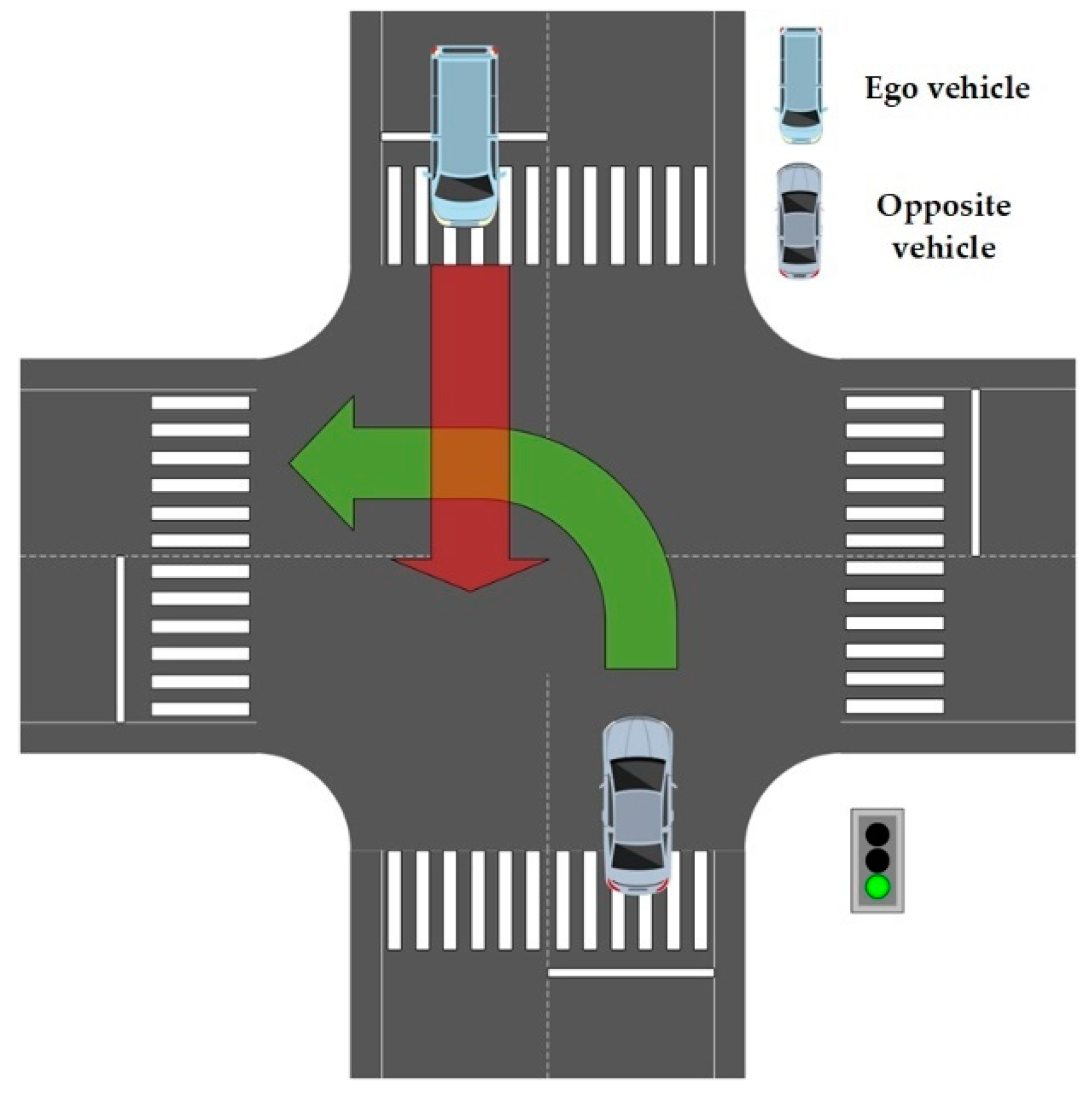
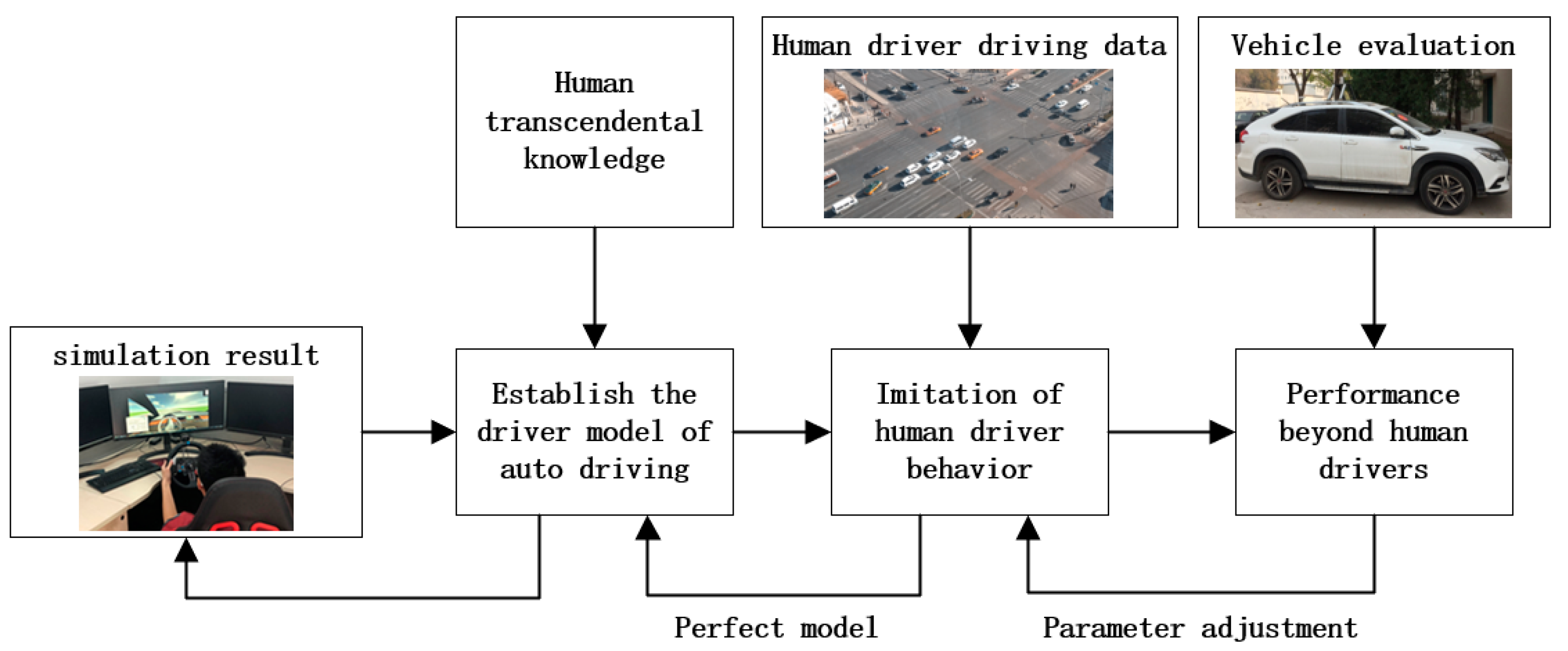
2.1. Humanoid Decision-Making Process at an Intersection
2.2. Scenario Evaluation
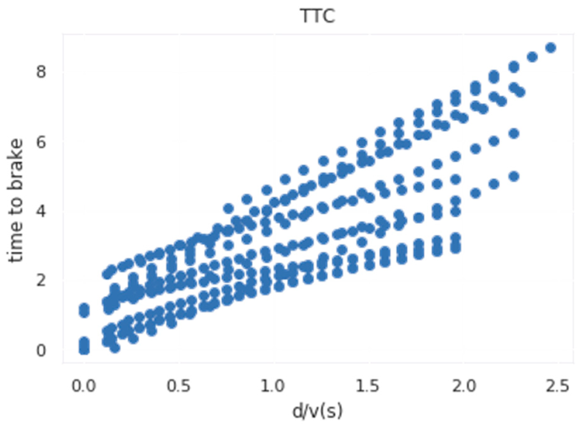
2.3. Time to Collision (TTC)
- : Distance between the test vehicle and the virtual collision point;
- : Speed of the test vehicle.
2.4. Semi-Markov Model
| Algorithm 1 SMDP Framework |
| In the planning window t: |
| If ( and ) |
| Then Execute cooperative strategy If () |
| Then Execute defensive strategies Else Execute general strategy |
2.5. Maximum Entropy Inverse Reinforcement Learning
2.6. Design of Evaluation Function
| Algorithm 2 Hierarchical Decision Model |
| Input: The status of the ego vehicle |
| If () |
| Then Execute evaluation function |
| Output: Series dynamics in planning window |
| If () |
| Then Execute evaluation function |
| Output: Series dynamics in planning window |
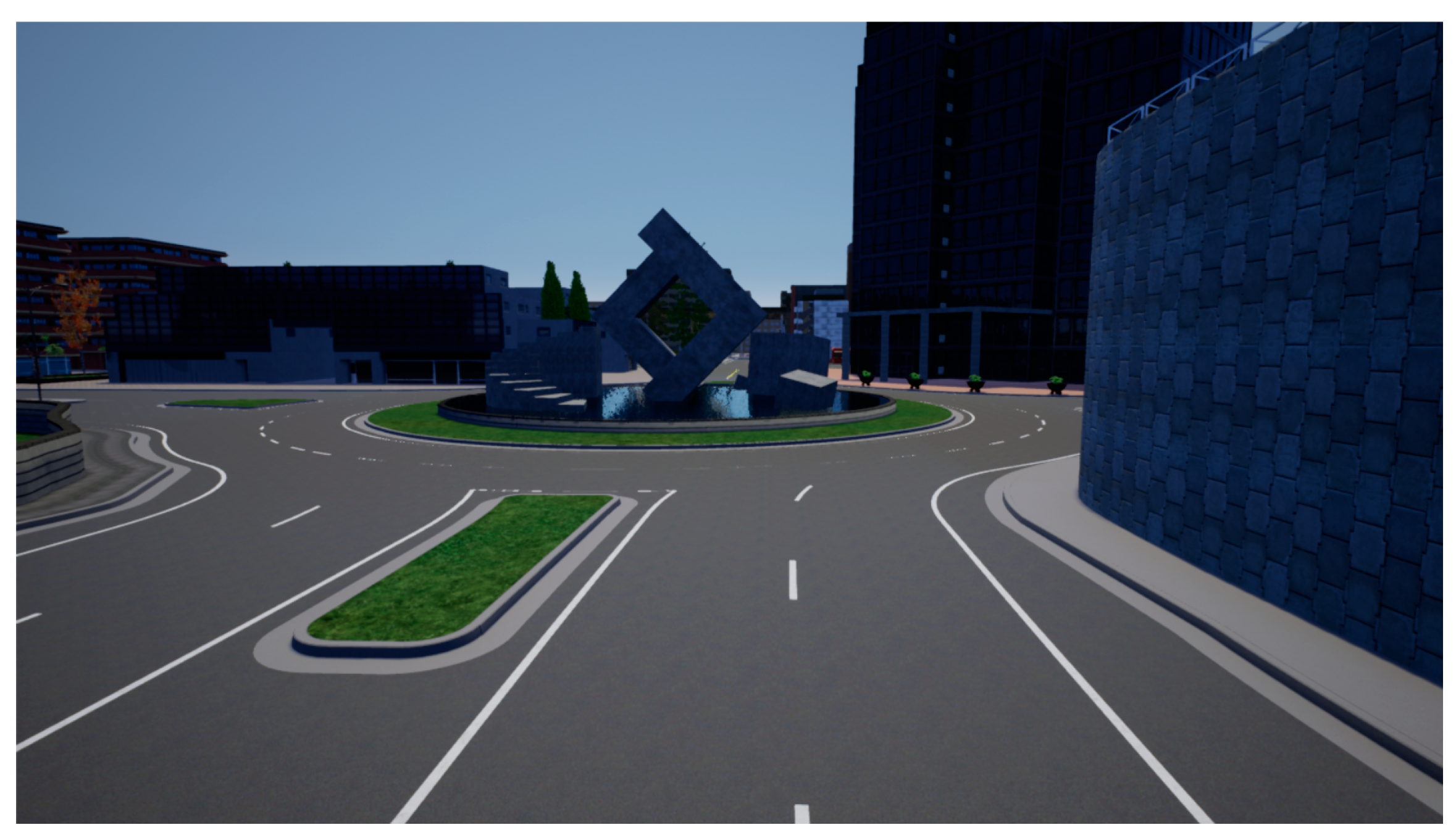
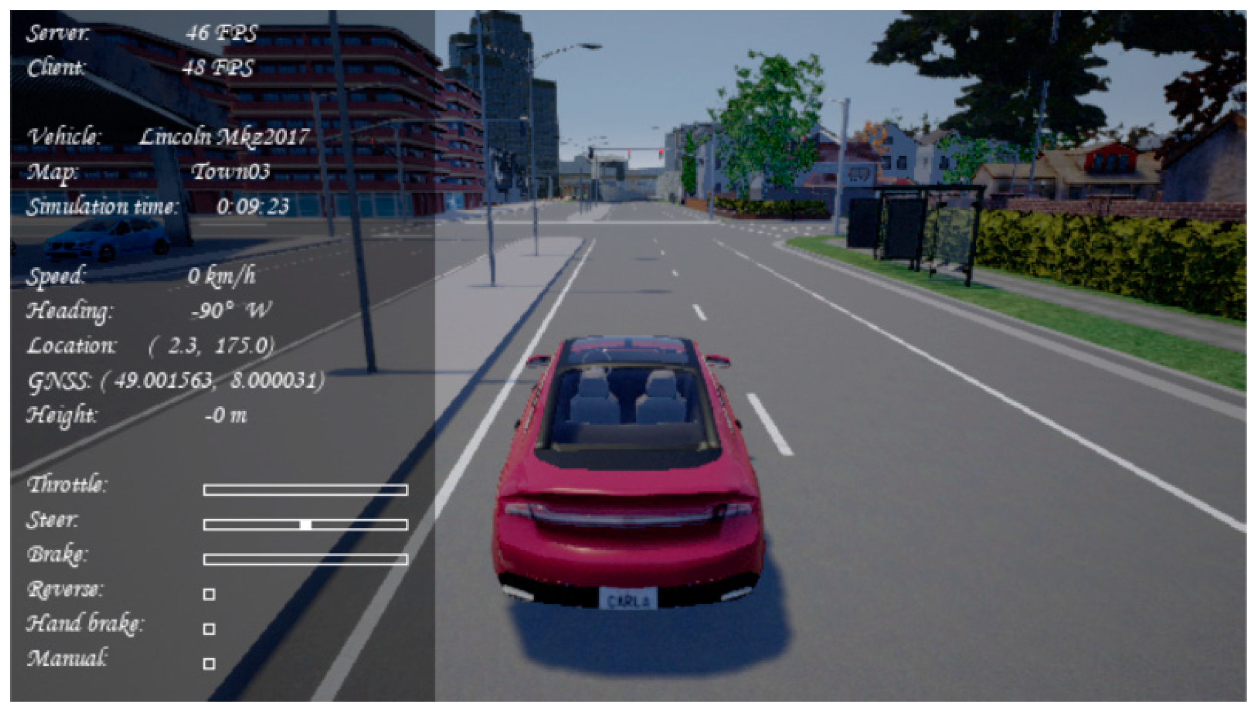
3. Simulation Scenario Verification
3.1. Scenario Design
3.2. Experimental Design
3.3. Scenario 1: The Opposite Vehicle Not Giving Way
3.4. Scenario 2: The Opposite Vehicle Giving Way
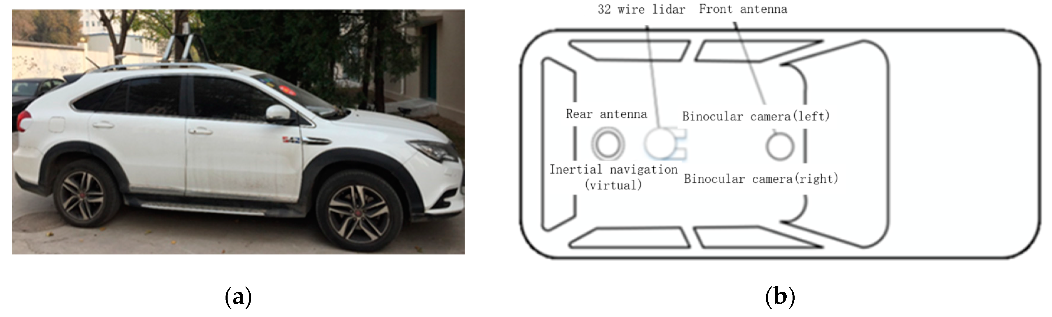
4. Real Vehicle Scenario Verification
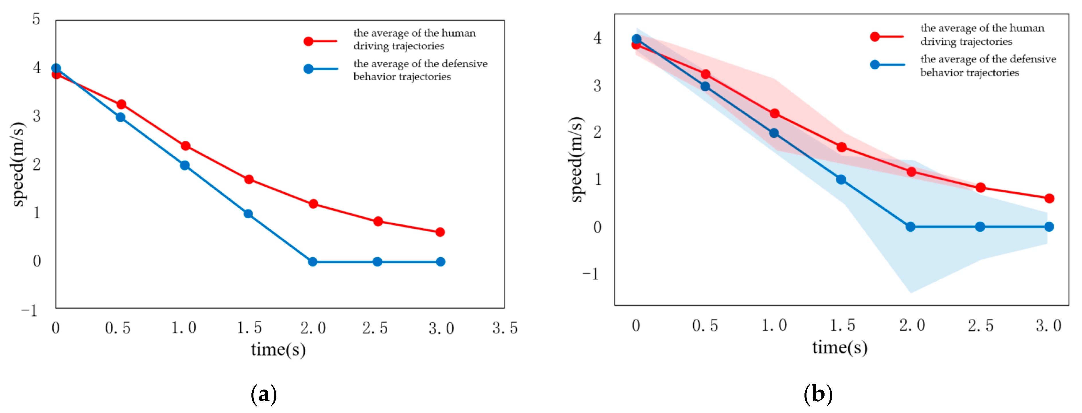
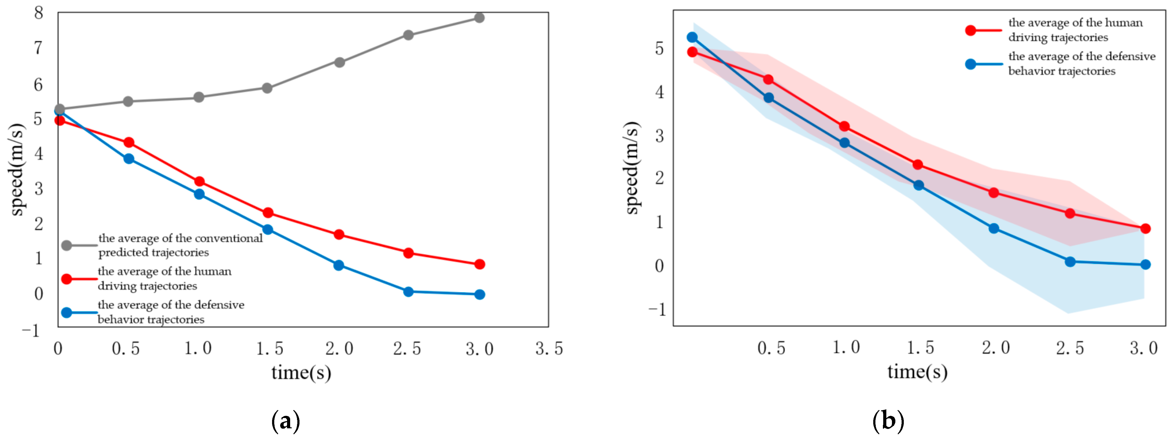
4.1. Scenario I
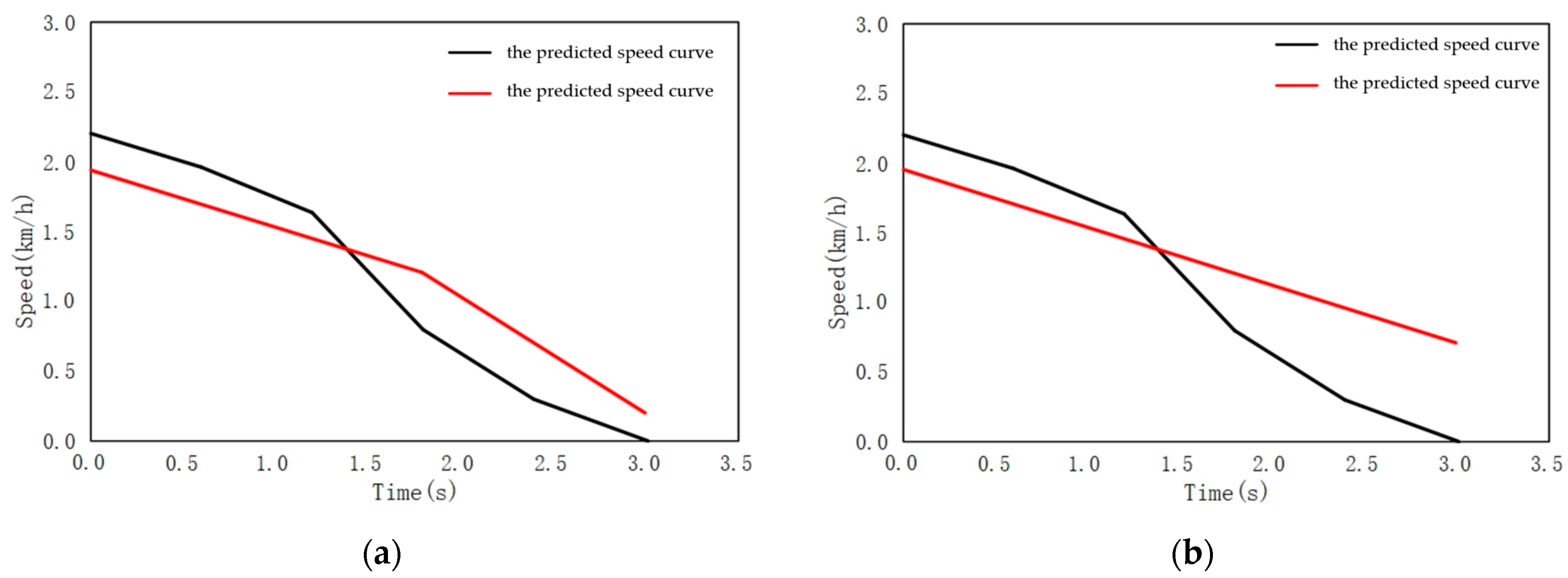
- (1)
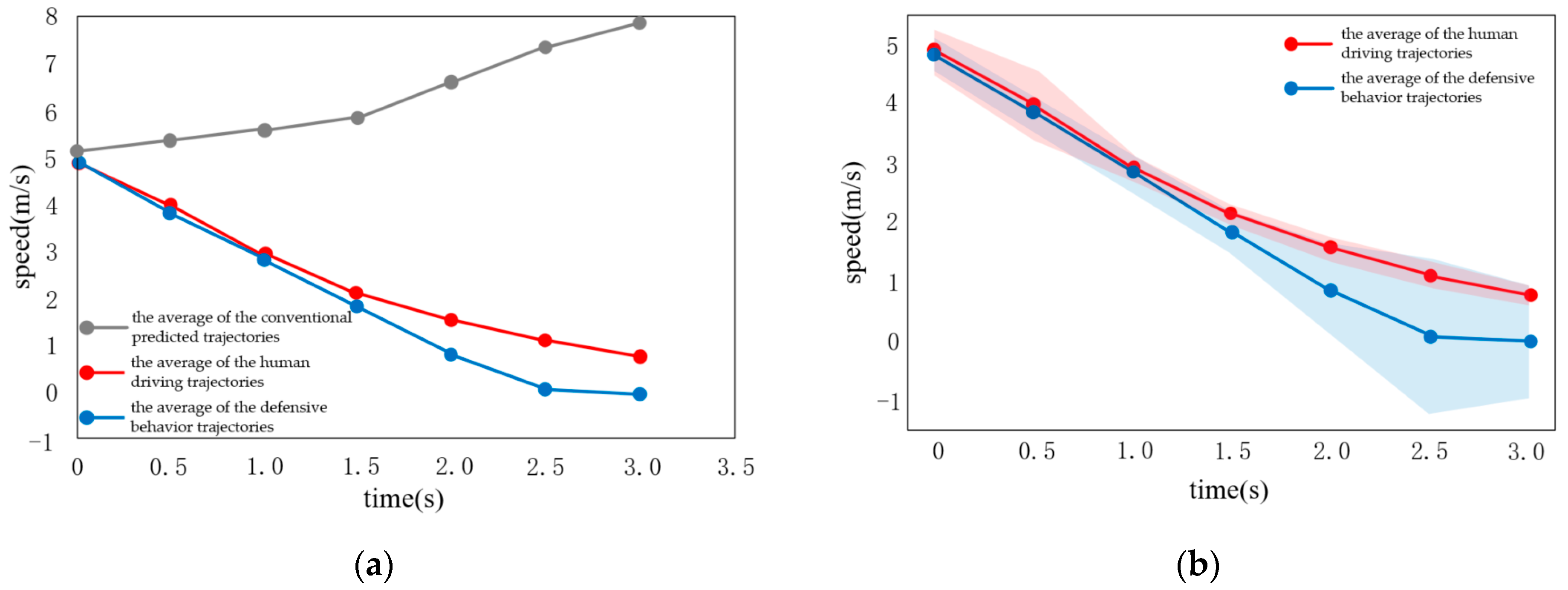
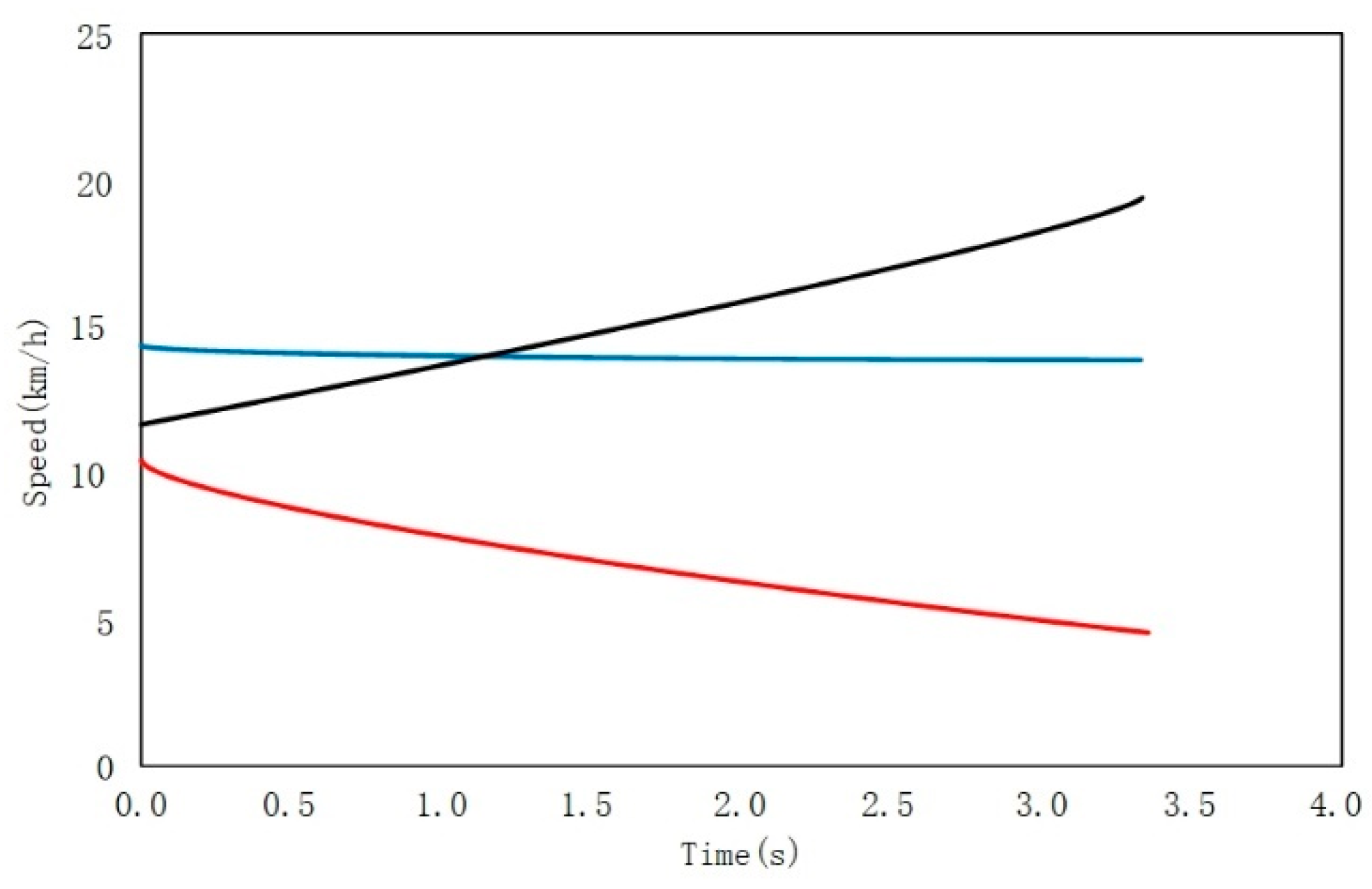
- Defensive behavior, similarly to human behavior, has a turning point in the middle of deceleration. The turning point of the vehicle speed curve decline is roughly consistent, indicating that human beings follow a rapid deceleration process, when approaching the conflict area. This shows that the learned defensive behavior is based on the defensive characteristics of human beings;
- (2)
- Defensive behavior actually achieves the defense effect by setting a safe area. Compared to conventional behavior, it still does not slow down to 0, when approaching the conflict area, which still poses a great risk of collision within the conflict area, indicating that setting a safe area can indeed achieve the effect of ensuring safety.
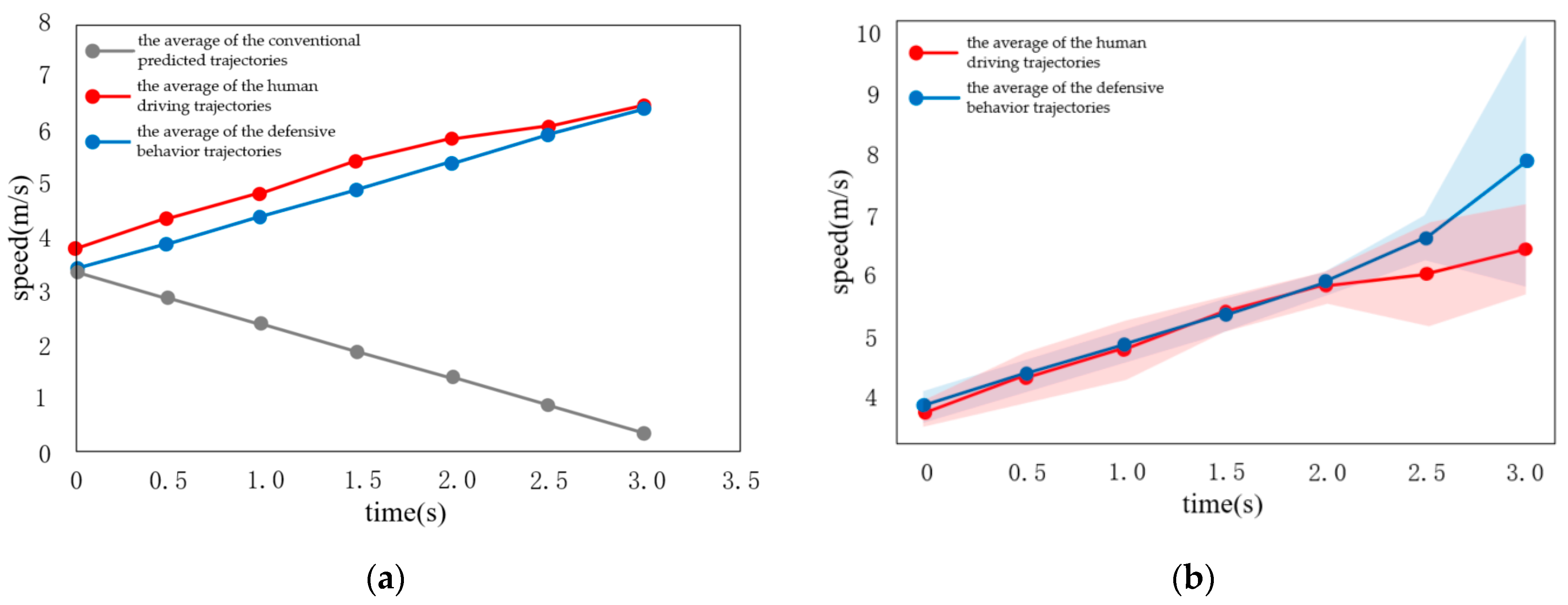
4.2. Scenario II
- (1)
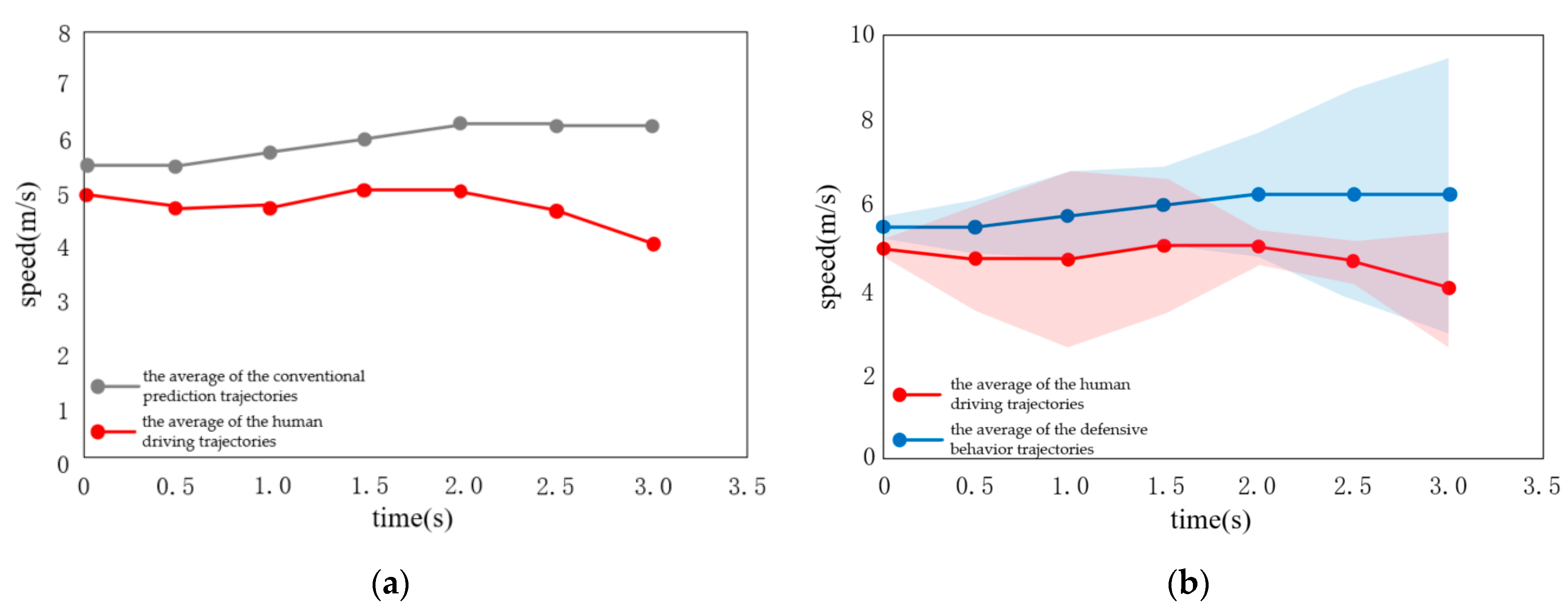
- Similar to human behavior, cooperative behavior has a turning point in the middle of acceleration. The turning point of the rising speed curve of the vehicle is roughly consistent, indicating that human beings follow a rapid acceleration process, when approaching the conflict area. It reflects the human response to the other vehicle avoidance behavior. This shows that, the learned cooperative behavior is based on the cooperative characteristics of human beings;
- (2)
- In fact, cooperative behavior means to leave the conflict area after 3 s. Conventional behavior is not based on the reward function. On the contrary, in order to avoid being too close to the obstacle, the vehicle is in the state of deceleration and gives way to the opposite vehicle, so it does not try to understand the intention of the opposite vehicle;
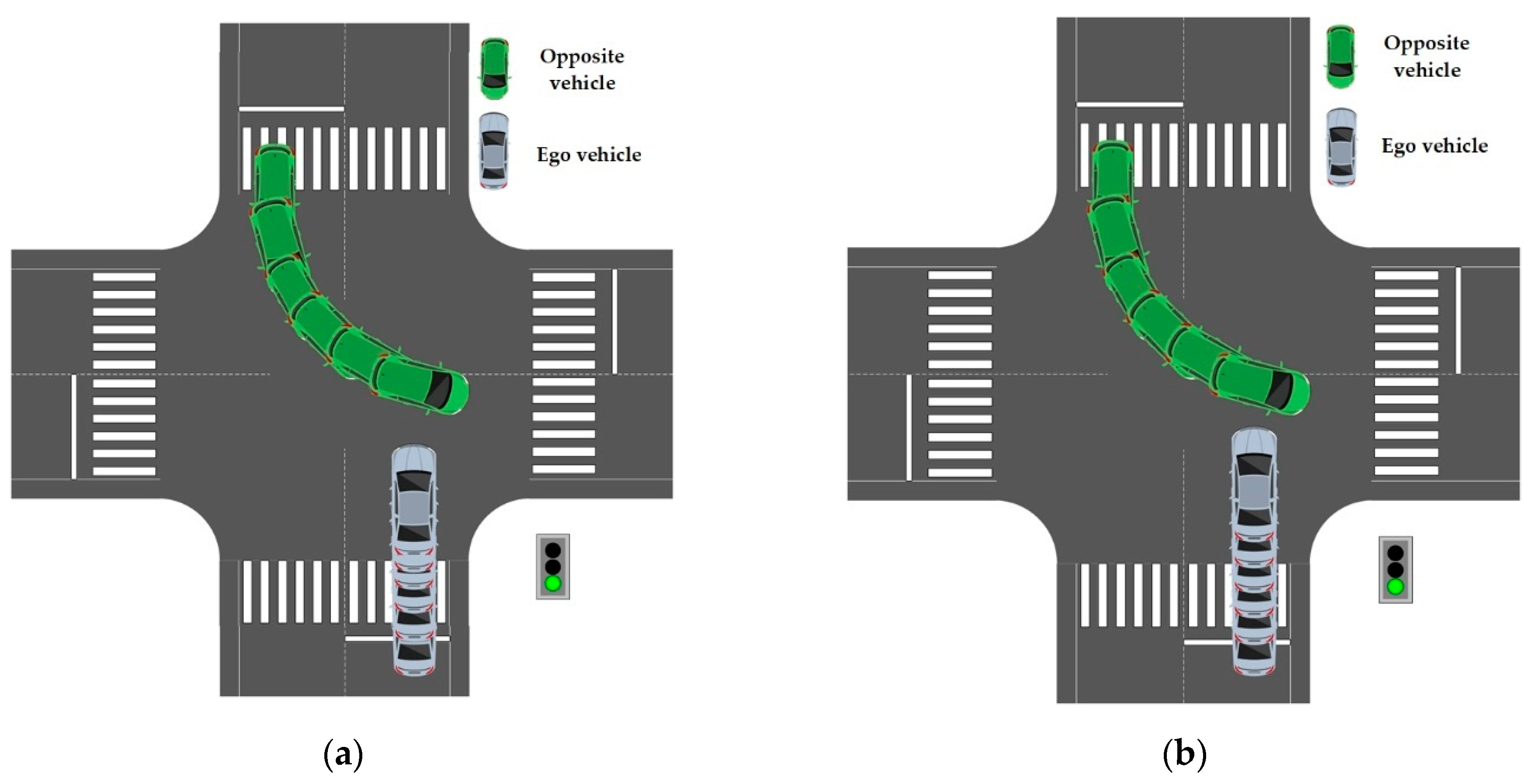
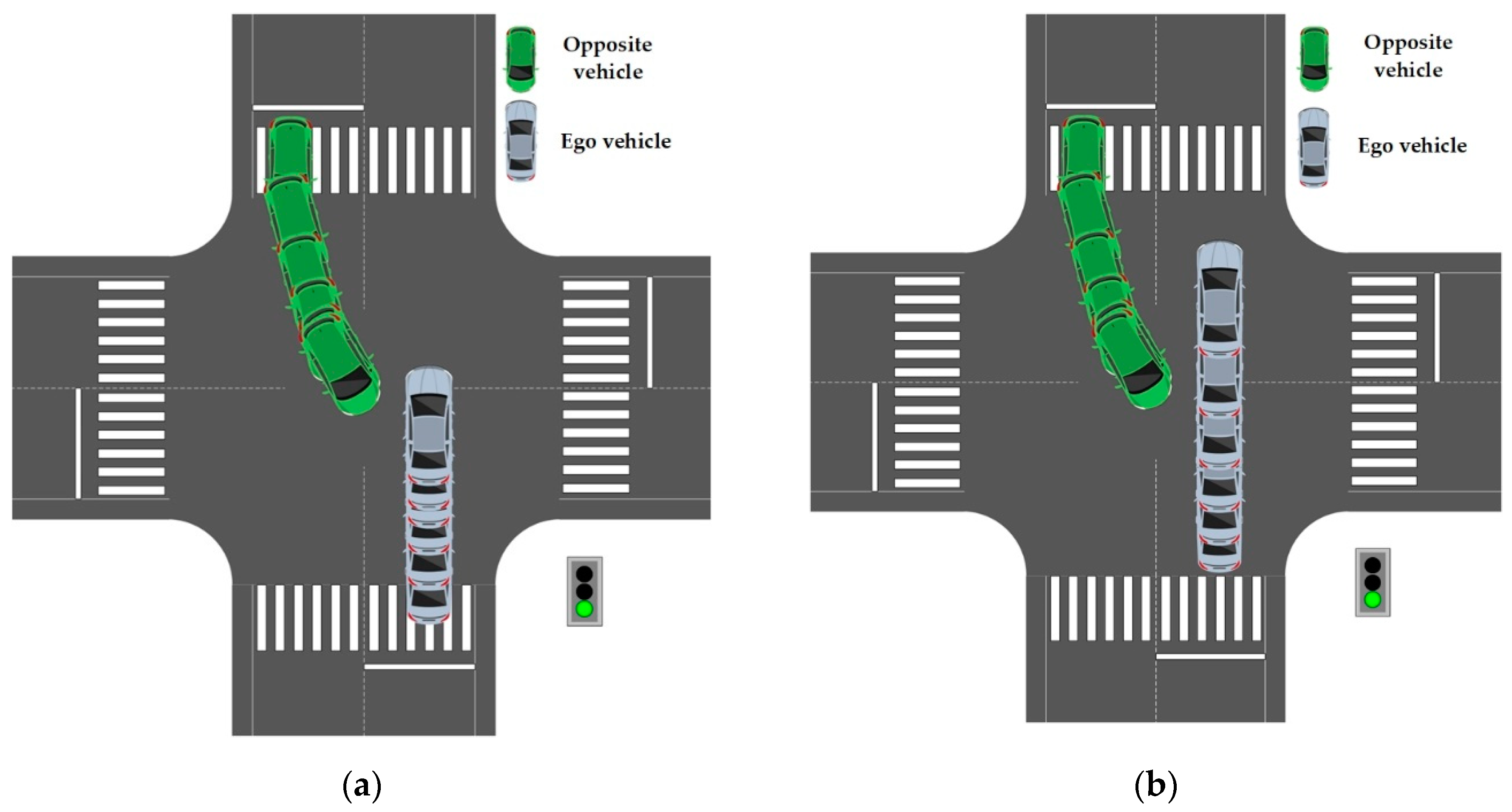
- (3)
- As shown in Figure 17, the blue vehicle is the test vehicle (ego vehicle) and the green vehicle is the opposite vehicle. The conventional behavior, compared to cooperative behavior, is not developed using the reward function, after constraining the vehicle to leave the conflict area for 3 s. Finally, it is quite far away from the opposite vehicle. In the environment of large traffic flow, parking arbitrarily at the intersection, in a way that other drivers do not understand, will put the vehicle in an extremely dangerous situation.
5. Conclusions
- (1)
- A human-like behavior decision-making method is proposed for decision-making in intersection scenarios. It is developed based on inverse reinforcement learning and semi-Markov model. The proposed method can learn well from demonstration trajectories of human experts, generating human-like trajectories;
- (2)
- The proposed model combines driving intention of other vehicles and ego vehicle, and uses the semi-Markov model to directly correspond the intention to the driving strategy, which adapts to the intention ambiguity of other vehicles in the real scene. Meanwhile, it abstracts the interaction behavior between other vehicles and ego vehicle into defensive behavior and cooperative behavior, and takes different behaviors for different scenarios;
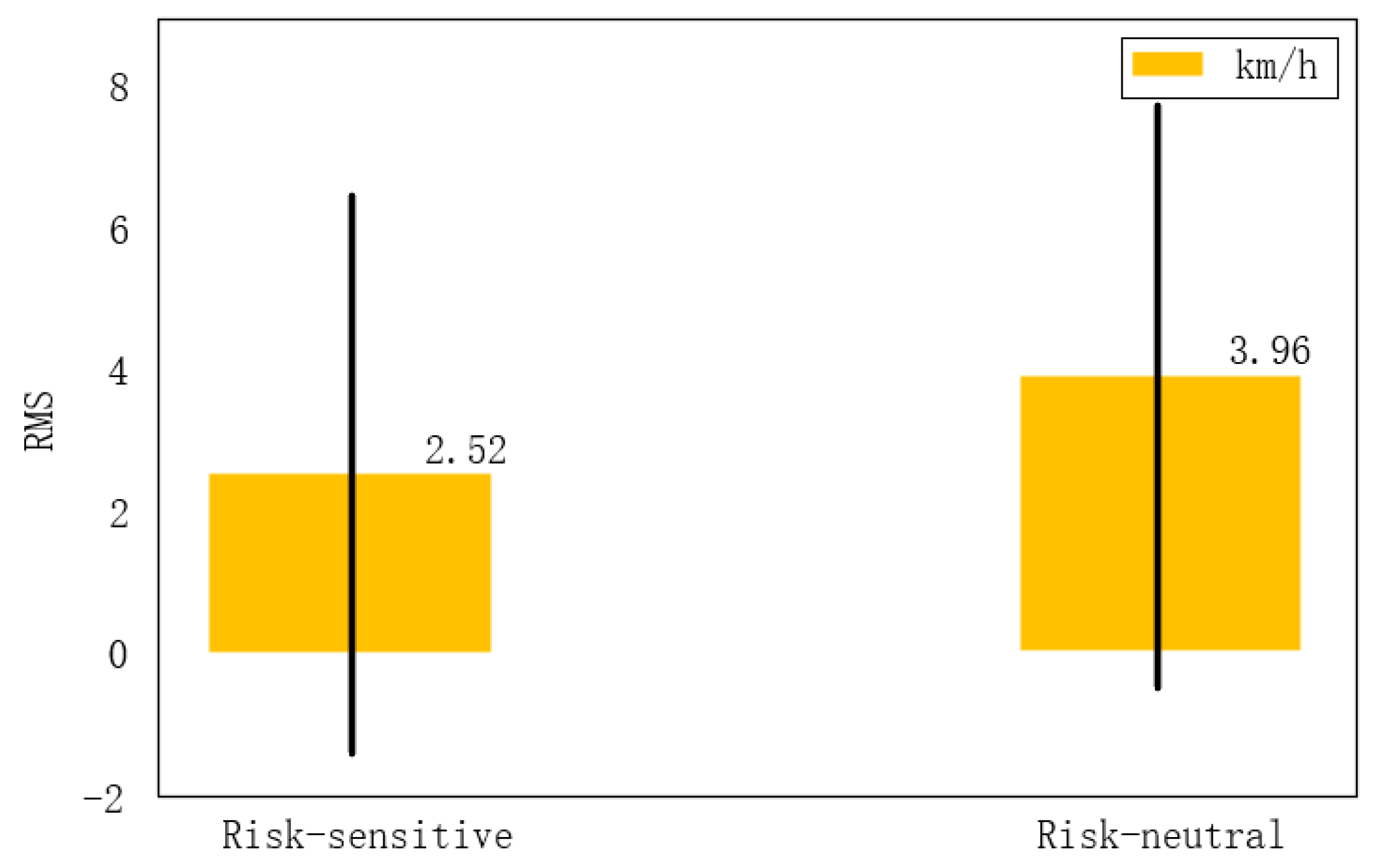
- (3)
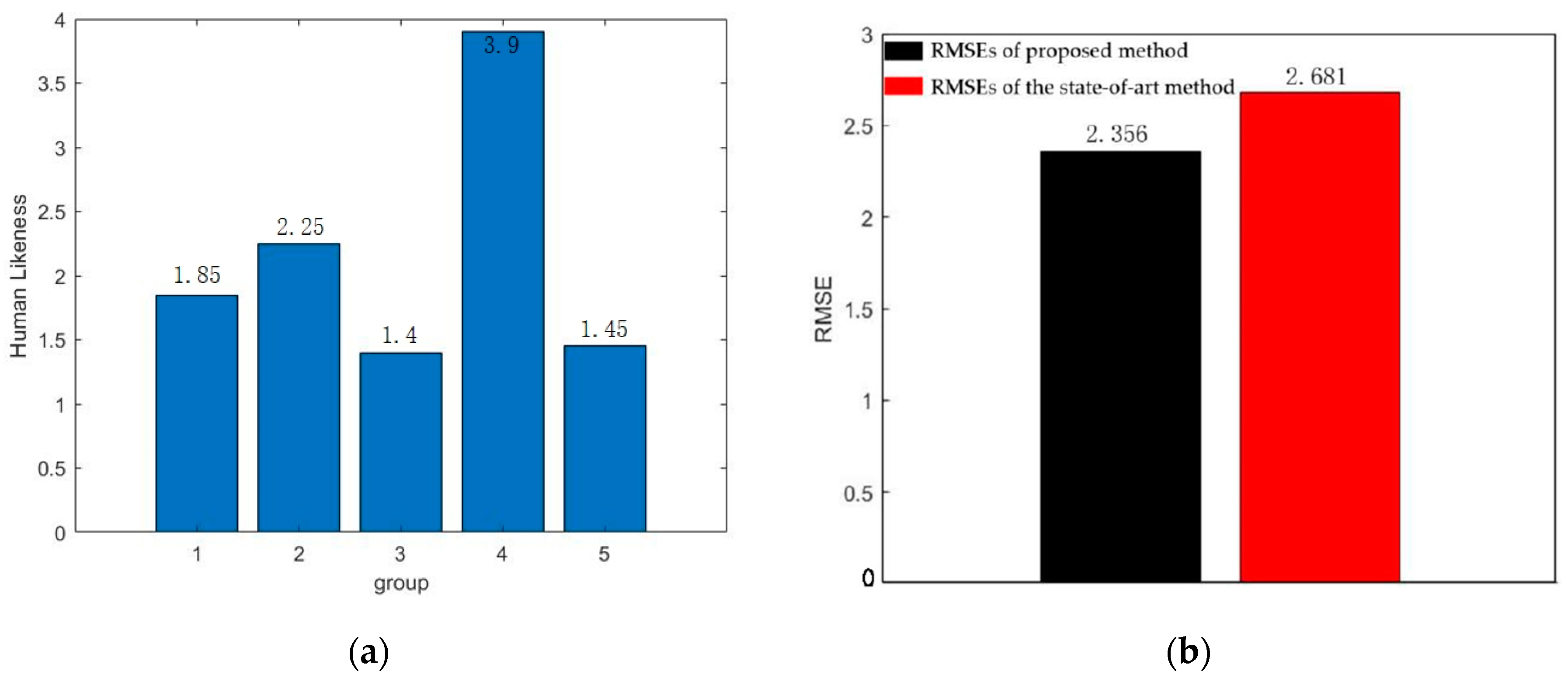
- Compared to traditional methods, the proposed method can learn well from human demonstration data, and is more in line with human driving behavior. The analysis results show that the method also has good stability, in addition with accuracy.
Author Contributions
Funding
Institutional Review Board Statement
Informed Consent Statement
Data Availability Statement
Conflicts of Interest
References
- Xia, Y.; Qu, Z.; Sun, Z.; Li, Z. A human-like model to understand surrounding vehicles’ lane changing intentions for autonomous driving. IEEE Trans. Veh. Technol. 2021, 70, 4178–4189. [Google Scholar] [CrossRef]
- Codevilla, F.; Müller, M.; López, A.; Koltun, V.; Dosovitskiy, A. End-to-end driving via conditional imitation learning. In Proceedings of the 2018 IEEE International Conference on Robotics and Automation (ICRA), Brisbane, QLD, Australia, 21–25 May 2018; pp. 4693–4700. [Google Scholar]
- Sheridan, T.B. Human–robot interaction: Status and challenges. Hum. Factors 2016, 58, 525–532. [Google Scholar] [CrossRef] [PubMed]
- Muir, H. Google Self-Driving Car Caught on Video Colliding with Bus. The Guardian. 2016. Available online: https://www.theguardian.com/technology/2016/mar/09/google-self-driving-car-crash-video-accident-bus (accessed on 12 May 2022).
- Li, L.; Ota, K.; Dong, M. Humanlike driving: Empirical decision-making system for autonomous vehicles. IEEE Trans. Veh. Technol. 2018, 67, 6814–6823. [Google Scholar] [CrossRef] [Green Version]
- Gu, Y.; Hashimoto, Y.; Hsu, L.; Iryo-Asano, M.; Kamijo, S. Human-like motion planning model for driving in signalized intersections. IATSS Res. 2017, 41, 129–139. [Google Scholar] [CrossRef] [Green Version]
- Emuna, R.; Borowsky, A.; Biess, A. Deep reinforcement learning for human-like driving policies in collision avoidance tasks of self-driving cars. arXiv 2020, arXiv:2006.04218. [Google Scholar]
- Hang, P.; Lv, C.; Xing, Y.; Huang, C.; Hu, Z. Human-like decision making for autonomous driving: A noncooperative game theoretic approach. IEEE Trans. Intell. Transp. 2020, 22, 2076–2087. [Google Scholar] [CrossRef]
- Hang, P.; Zhang, Y.; Lv, C. Interacting with Human Drivers: Human-like Driving and Decision Making for Autonomous Vehicles. arXiv 2022, arXiv:2201.03125. [Google Scholar]
- Guo, C.; Kidono, K.; Machida, T.; Terashima, R.; Kojima, Y. Human-like behavior generation for intelligent vehicles in urban environment based on a hybrid potential map. In Proceedings of the 2017 IEEE Intelligent Vehicles Symposium (IV), Los Angeles, CA, USA, 11–14 June 2017; pp. 197–203. [Google Scholar]
- Naumann, M.; Lauer, M.; Stiller, C. Generating comfortable, safe and comprehensible trajectories for automated vehicles in mixed traffic. In Proceedings of the 2018 21st International Conference on Intelligent Transportation Systems (ITSC), Maui, HI, USA, 4–7 November 2018; pp. 575–582. [Google Scholar]
- Sharath, M.N.; Velaga, N.R.; Quddus, M. 2-dimensional human-like driver model for autonomous vehicles in mixed traffic. IET Intell. Transp. Syst. 2020, 14, 1913–1922. [Google Scholar] [CrossRef]
- Al-Shihabi, T.; Mourant, R.R. A framework for modeling human-like driving behaviors for autonomous vehicles in driving simulators. In Proceedings of the fifth International Conference on Autonomous Agents, Montreal, QC, Canada, 28 May–1 June 2001; pp. 286–291. [Google Scholar]
- Cheng, S.; Song, J.; Fang, S. A universal control scheme of human-like steering in multiple driving scenarios. IEEE Trans. Intell. Transp. 2020, 22, 3135–3145. [Google Scholar] [CrossRef]
- Wei, C.; Paschalidis, E.; Merat, N.; Solernou, A.; Hajiseyedjavadi, F.; Romano, R. Human-like Decision Making and Motion Control for Smooth and Natural Car Following. IEEE Trans. Intell. Veh. 2021. [Google Scholar] [CrossRef]
- Ulbrich, S.; Maurer, M. Probabilistic online POMDP decision making for lane changes in fully automated driving. In Proceedings of the 16th International IEEE Conference on Intelligent Transportation Systems (ITSC 2013), The Hague, The Netherlands, 6–9 October 2013; pp. 2063–2067. [Google Scholar]
- Cheng, W.; Wang, G.; Wu, S.; Xiong, G.; Gong, J. A human-like longitudinal decision model of intelligent vehicle at signalized intersections. In Proceedings of the 2017 IEEE International Conference on Real-time Computing and Robotics (RCAR), Okinawa, Japan, 14–18 July 2017; pp. 415–420. [Google Scholar]
- Lin, X.; Zhang, J.; Shang, J.; Wang, Y.; Yu, H.; Zhang, X. Decision making through occluded intersections for autonomous driving. In Proceedings of the 2019 IEEE Intelligent Transportation Systems Conference (ITSC), Auckland, New Zealand, 27–30 October 2019; pp. 2449–2455. [Google Scholar]
- Oh, K.; Oh, S.; Lee, J.; Yi, K. Development of a Human-Like Learning Frame for Data-Driven Adaptive Control Algorithm of Automated Driving. In Proceedings of the 2021 21st International Conference on Control, Automation and Systems (ICCAS), Jeju, Korea, 12–15 October 2021; pp. 1737–1741. [Google Scholar]
- Wu, J.; Huang, Z.; Huang, C.; Hu, Z.; Hang, P.; Xing, Y.; Lv, C. Human-in-the-loop deep reinforcement learning with application to autonomous driving. arXiv 2021, arXiv:2104.07246. [Google Scholar]
- Xu, D.; Ding, Z.; He, X.; Zhao, H.; Moze, M.; Aioun, F.; Guillemard, F. Learning from naturalistic driving data for human-like autonomous highway driving. IEEE Trans. Intell. Transp. 2020, 22, 7341–7354. [Google Scholar] [CrossRef]
- Sun, T.; Gao, Z.; Gao, F.; Zhang, T.; Chen, S.; Zhao, K. A brain-inspired decision-making linear neural network and its application in automatic drive. Sensors 2021, 21, 794. [Google Scholar] [CrossRef] [PubMed]
- Grigorescu, S.; Trasnea, B.; Cocias, T.; Macesanu, G. A survey of deep learning techniques for autonomous driving. J. Field Robot. 2020, 37, 362–386. [Google Scholar] [CrossRef]
- Xie, J.; Xu, X.; Wang, F.; Jiang, H. Modeling human-like longitudinal driver model for intelligent vehicles based on reinforcement learning. Proc. Inst. Mech. Eng. Part D J. Autom. Eng. 2021, 235, 2226–2241. [Google Scholar] [CrossRef]
- Zhu, M.; Wang, X.; Wang, Y. Human-like autonomous car-following model with deep reinforcement learning. Transp. Res. Part C Emerg. Technol. 2018, 97, 348–368. [Google Scholar] [CrossRef] [Green Version]
- Zhang, Y.; Sun, P.; Yin, Y.; Lin, L.; Wang, X. Human-like autonomous vehicle speed control by deep reinforcement learning with double Q-learning. In Proceedings of the 2018 IEEE Intelligent Vehicles Symposium (IV), Changshu, China, 26–30 June 2018; pp. 1251–1256. [Google Scholar]
- Sama, K.; Morales, Y.; Liu, H.; Akai, N.; Carballo, A.; Takeuchi, E.; Takeda, K. Extracting human-like driving behaviors from expert driver data using deep learning. IEEE Trans. Veh. Technol. 2020, 69, 9315–9329. [Google Scholar] [CrossRef]
- Hecker, S.; Dai, D.; Van Gool, L. Learning accurate, comfortable and human-like driving. arXiv 2019, arXiv:1903.10995. [Google Scholar]
- Lu, C.; Gong, J.; Lv, C.; Chen, X.; Cao, D.; Chen, Y. A personalized behavior learning system for human-like longitudinal speed control of autonomous vehicles. Sensors 2019, 19, 3672. [Google Scholar] [CrossRef] [Green Version]
- Chen, J.; Li, S.E.; Tomizuka, M. Interpretable end-to-end urban autonomous driving with latent deep reinforcement learning. arXiv 2020, arXiv:2001.08726. [Google Scholar] [CrossRef]
- Amini, A.; Gilitschenski, I.; Phillips, J.; Moseyko, J.; Banerjee, R.; Karaman, S.; Rus, D. Learning robust control policies for end-to-end autonomous driving from data-driven simulation. IEEE Robot. Autom. Lett. 2020, 5, 1143–1150. [Google Scholar] [CrossRef]
- Huang, Z.; Lv, C.; Xing, Y.; Wu, J. Multi-modal sensor fusion-based deep neural network for end-to-end autonomous driving with scene understanding. IEEE Sens. J. 2020, 21, 11781–11790. [Google Scholar] [CrossRef]
- Chen, S.; Wang, M.; Song, W.; Yang, Y.; Li, Y.; Fu, M. Stabilization approaches for reinforcement learning-based end-to-end autonomous driving. IEEE Trans. Veh. Technol. 2020, 69, 4740–4750. [Google Scholar] [CrossRef]
- Tampuu, A.; Matiisen, T.; Semikin, M.; Fishman, D.; Muhammad, N. A survey of end-to-end driving: Architectures and training methods. arXiv 2020, arXiv:2003.06404. [Google Scholar] [CrossRef]
- Abbeel, P.; Ng, A.Y. Apprenticeship learning via inverse reinforcement learning. In Proceedings of the twenty-First International Conference on Machine Learning, Banff, AB, Canada, 4–8 July 2004; p. 1. [Google Scholar]
- Ziebart, B.D.; Maas, A.L.; Bagnell, J.A.; Dey, A.K. Maximum entropy inverse reinforcement learning. In Proceedings of the Twenty-Third AAAI Conference on Artificial Intelligence, Chicago, IL, USA, 13–17 July 2008; pp. 1433–1438. [Google Scholar]
- Kuderer, M.; Gulati, S.; Burgard, W. Learning driving styles for autonomous vehicles from demonstration. In Proceedings of the 2015 IEEE International Conference on Robotics and Automation (ICRA), Seattle, WA, USA, 26–30 May 2015; pp. 2641–2646. [Google Scholar]
- Levine, S.; Koltun, V. Continuous inverse optimal control with locally optimal examples. arXiv 2012, arXiv:1206.4617. [Google Scholar]
- Naumann, M.; Sun, L.; Zhan, W.; Tomizuka, M. Analyzing the suitability of cost functions for explaining and imitating human driving behavior based on inverse reinforcement learning. In Proceedings of the 2020 IEEE International Conference on Robotics and Automation (ICRA), Paris, France, 31 May–31 August 2020; pp. 5481–5487. [Google Scholar]
- Huang, Z.; Wu, J.; Lv, C. Driving behavior modeling using naturalistic human driving data with inverse reinforcement learning. IEEE Trans. Intell. Transp. Syst. 2021. [Google Scholar] [CrossRef]
- Le Mero, L.; Yi, D.; Dianati, M.; Mouzakitis, A. A survey on imitation learning techniques for end-to-end autonomous vehicles. IEEE Trans. Intell. Transp. 2022. [Google Scholar] [CrossRef]
- McAllister, R.; Gal, Y.; Kendall, A.; Van Der Wilk, M.; Shah, A.; Cipolla, R.; Weller, A. Concrete problems for autonomous vehicle safety: Advantages of Bayesian deep learning. In Proceedings of the Twenty-Sixth International Joint Conference on Artificial Intelligence (IJCAI-17), Melbourne, Australia, 19–25 August 2017. [Google Scholar]
- Noh, S. Decision-making framework for autonomous driving at road intersections: Safeguarding against collision, overly conservative behavior, and violation vehicles. IEEE Trans. Ind. Electron. 2018, 66, 3275–3286. [Google Scholar] [CrossRef]
- Kaempchen, N.; Schiele, B.; Dietmayer, K. Situation assessment of an autonomous emergency brake for arbitrary vehicle-to-vehicle collision scenarios. IEEE Trands. Intell. Transp. 2009, 10, 678–687. [Google Scholar] [CrossRef]
- Kumar, A.S.B.; Modh, A.; Babu, M.; Gopalakrishnan, B.; Krishna, K.M. A novel lane merging framework with probabilistic risk based lane selection using time scaled collision cone. In Proceedings of the 2018 IEEE Intelligent Vehicles Symposium (IV), Changshu, China, 26–30 June 2018; pp. 1406–1411. [Google Scholar]
- de Campos, G.R.; Falcone, P.; Hult, R.; Wymeersch, H.; Sjöberg, J. Traffic coordination at road intersections: Autonomous decision-making algorithms using model-based heuristics. IEEE Intell. Transp. Syst. Mag. 2017, 9, 8–21. [Google Scholar] [CrossRef] [Green Version]
- Dietterich, T.G. Hierarchical reinforcement learning with the MAXQ value function decomposition. J. Artif. Intell. Res. 2000, 13, 227–303. [Google Scholar] [CrossRef] [Green Version]
- Bradtke, S.; Duff, M. Reinforcement learning methods for continuous-time Markov decision problems. Adv. Neural Inf. Process. Syst. 1994, 7, 1162–1165. [Google Scholar]
- Qiao, Z.; Muelling, K.; Dolan, J.; Palanisamy, P.; Mudalige, P. Pomdp and hierarchical options mdp with continuous actions for autonomous driving at intersections. In Proceedings of the 2018 21st International Conference on Intelligent Transportation Systems (ITSC), Maui, HI, USA, 4–7 November 2018; pp. 2377–2382. [Google Scholar]
- Ng, A.Y.; Russell, S.J. Algorithms for Inverse Reinforcement Learning. In Proceedings of the International Conference on Machine Learning (ICML), San Francisco, CA, USA, 29 June–2 July 2000; pp. 663–670. [Google Scholar]
- Moehle, N. Risk-Sensitive Model Predictive Control. arXiv 2021, arXiv:2101.11166. [Google Scholar]
- Urpí, N.A.; Curi, S.; Krause, A. Risk-averse offline reinforcement learning. arXiv 2021, arXiv:2102.05371. [Google Scholar]
- Di Filippo, I. Can Risk Aversion Improve the Efficiency of Traffic networks? A Comparison between Risk Neutral and Risk Averse Routing Games. Bachelor’s Thesis, Luiss Guido Carli, Rome, Italy, 2021. [Google Scholar]
- Lu, C.; Lv, C.; Gong, J.; Wang, W.; Cao, D.; Wang, F. Instance-Level Knowledge Transfer for Data-Driven Driver Model Adaptation with Homogeneous Domains. IEEE Trans. Intell. Transp. Syst. 2022. [Google Scholar] [CrossRef]


| Category | ||||
|---|---|---|---|---|
| 1.000 | 0.834 | −0.104 | 0.9178 | |
| (m/s) | 0.834 | 1.000 | 0.038 | 0.978 |
| (m) | −0.104 | 0.038 | 1.000 | −0.054 |
| 0.918 | 0.978 | −0.054 | 1.000 |
| Average of Age (Years) | Standard Deviation of Age | Average of Driving Experience | Standard Deviation of Driving Experience (Years) |
|---|---|---|---|
| 24.43 | 1.40 | 4.43 | 1.76 |
| Situation | |||
|---|---|---|---|
| Danger | 47.677 | 0.198 | 1 |
| Security | 4.56 | 13.09 | 1 |
| Risk neutral | 9.45 | 2.09 | 1 |
Publisher’s Note: MDPI stays neutral with regard to jurisdictional claims in published maps and institutional affiliations. |
© 2022 by the authors. Licensee MDPI, Basel, Switzerland. This article is an open access article distributed under the terms and conditions of the Creative Commons Attribution (CC BY) license (https://creativecommons.org/licenses/by/4.0/).
Share and Cite
Wu, Z.; Qu, F.; Yang, L.; Gong, J. Human-like Decision Making for Autonomous Vehicles at the Intersection Using Inverse Reinforcement Learning. Sensors 2022, 22, 4500. https://doi.org/10.3390/s22124500
Wu Z, Qu F, Yang L, Gong J. Human-like Decision Making for Autonomous Vehicles at the Intersection Using Inverse Reinforcement Learning. Sensors. 2022; 22(12):4500. https://doi.org/10.3390/s22124500
Chicago/Turabian StyleWu, Zheng, Fangbing Qu, Lin Yang, and Jianwei Gong. 2022. "Human-like Decision Making for Autonomous Vehicles at the Intersection Using Inverse Reinforcement Learning" Sensors 22, no. 12: 4500. https://doi.org/10.3390/s22124500
APA StyleWu, Z., Qu, F., Yang, L., & Gong, J. (2022). Human-like Decision Making for Autonomous Vehicles at the Intersection Using Inverse Reinforcement Learning. Sensors, 22(12), 4500. https://doi.org/10.3390/s22124500