
Coupling Interference between Eddy Current Sensors for the Radial Displacement Measurement of a Cylindrical Target


Abstract
:1. Introduction
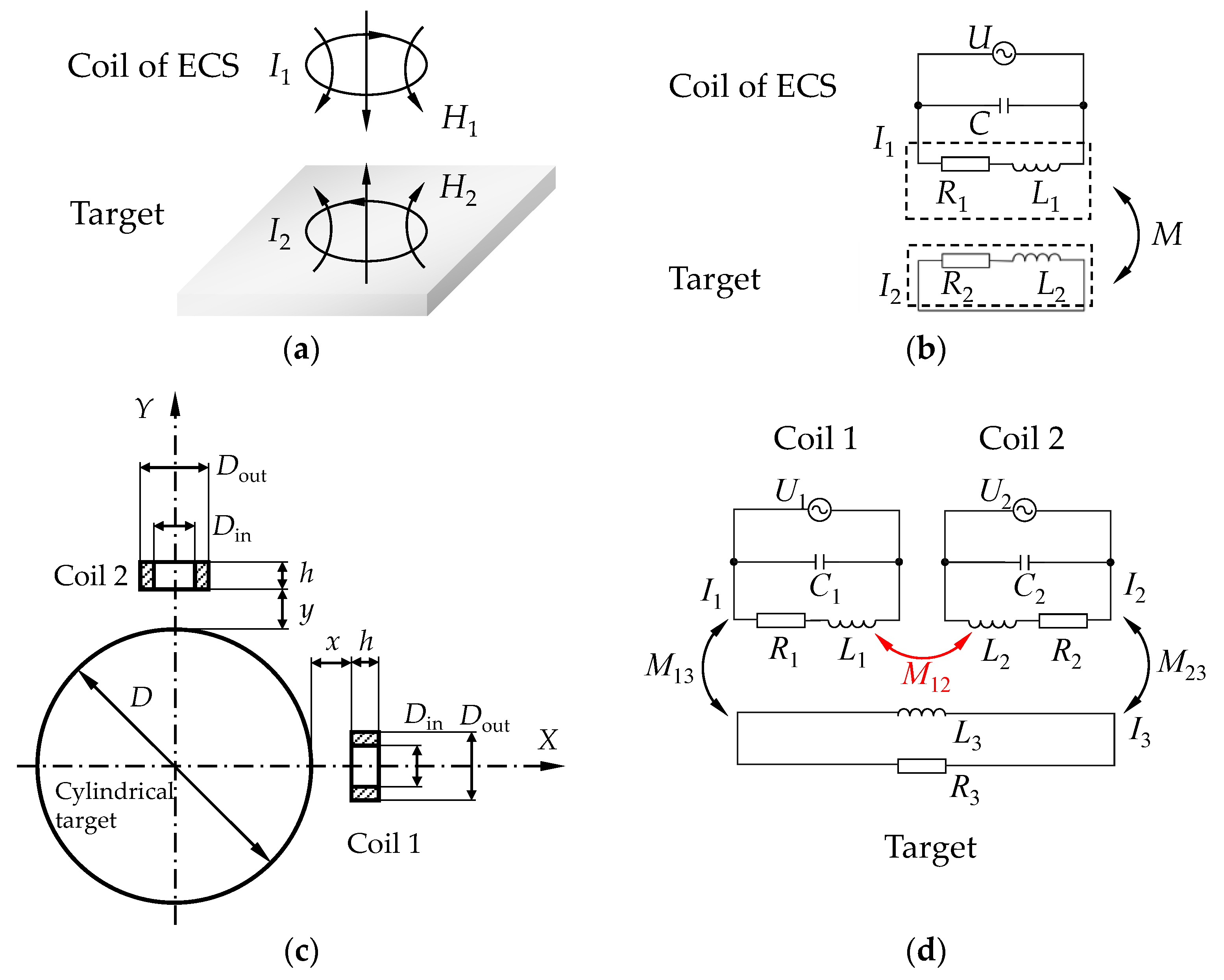
2. Basic Principle
3. Simulation Analyses
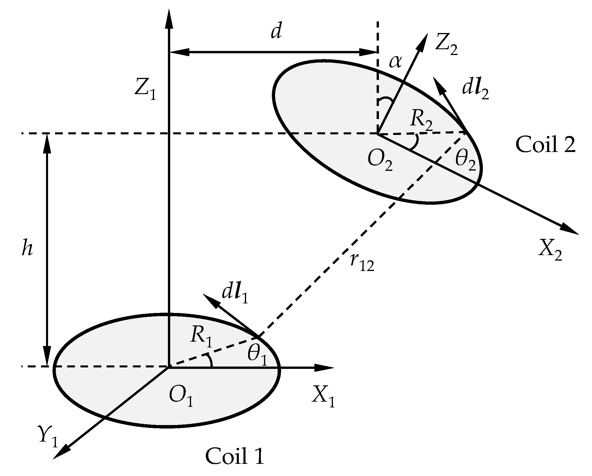
3.1. Theories of the Mutual Inductance of Two Coils
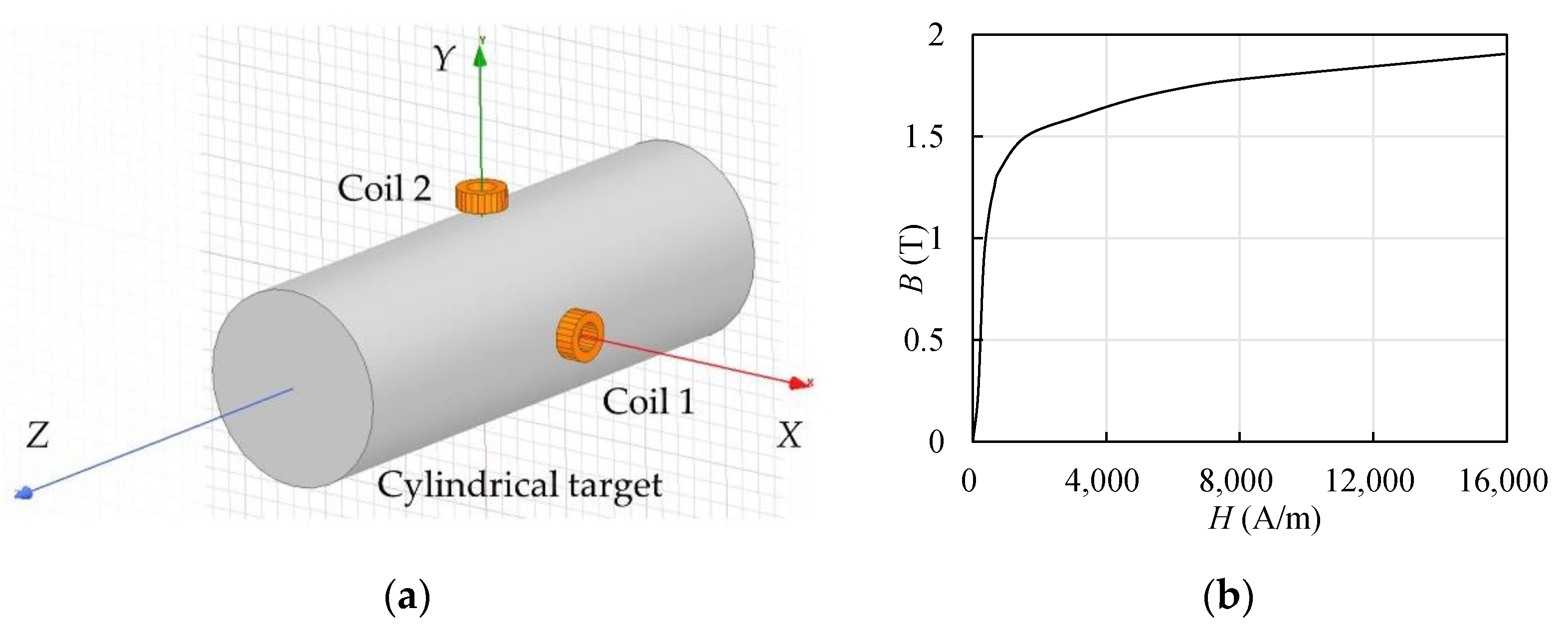
3.2. FEM Simulation Modeling
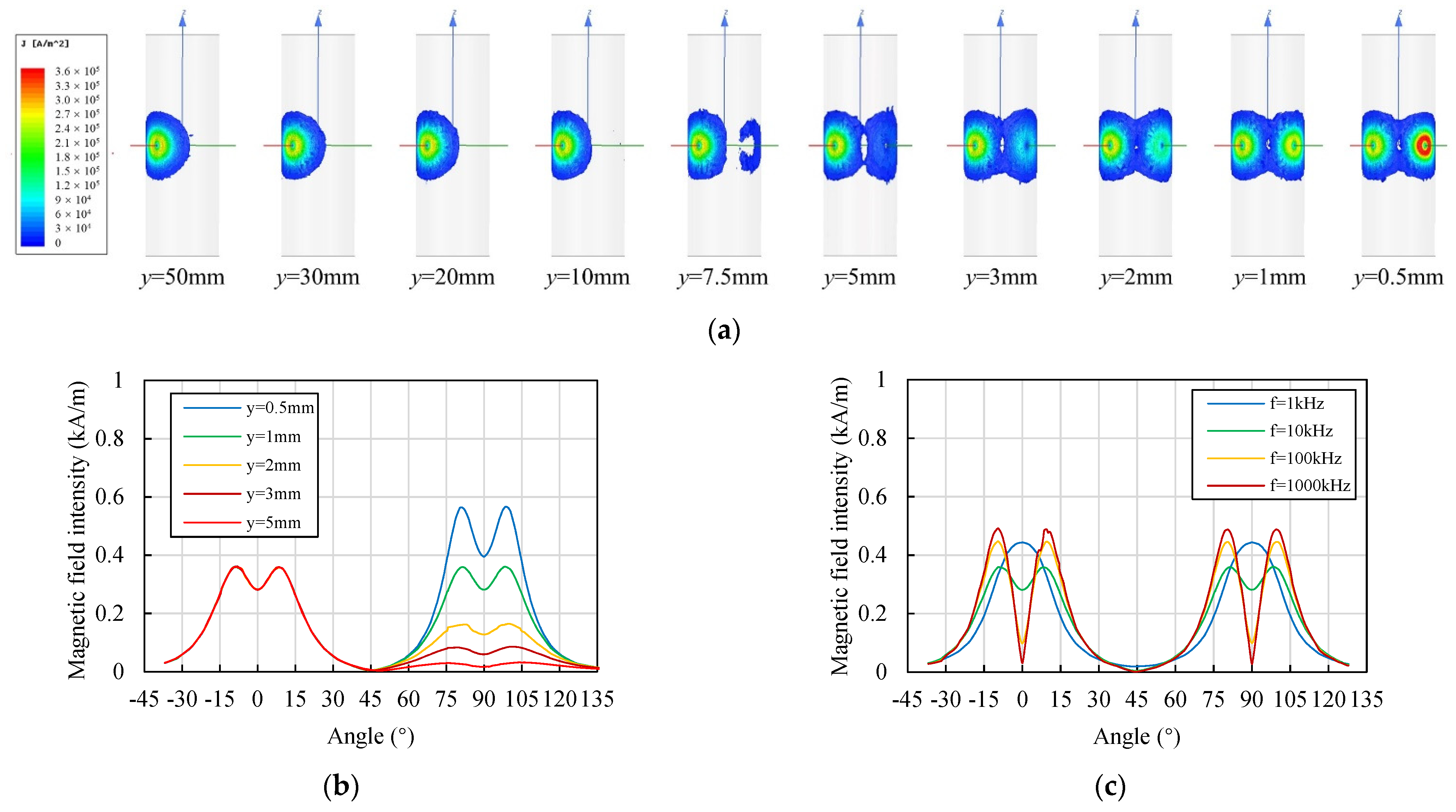
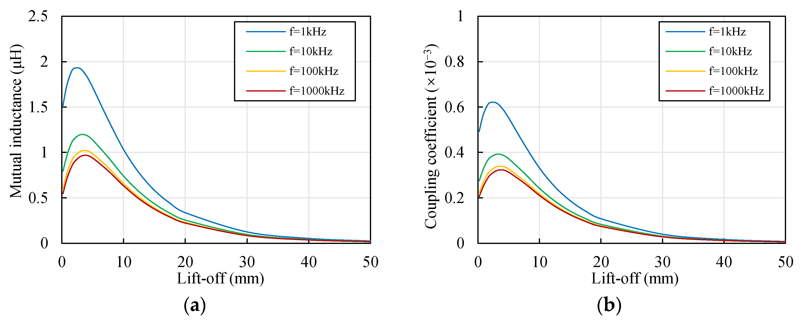
3.3. Influence of Lift-Off on Coupling Effect
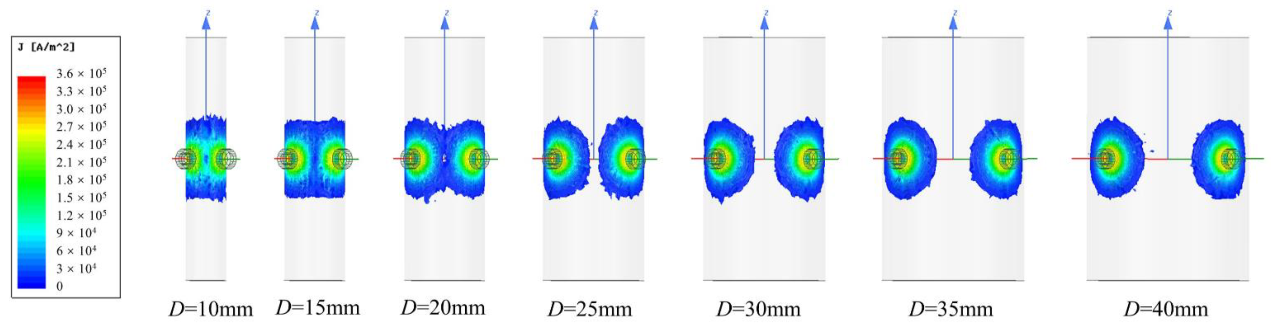
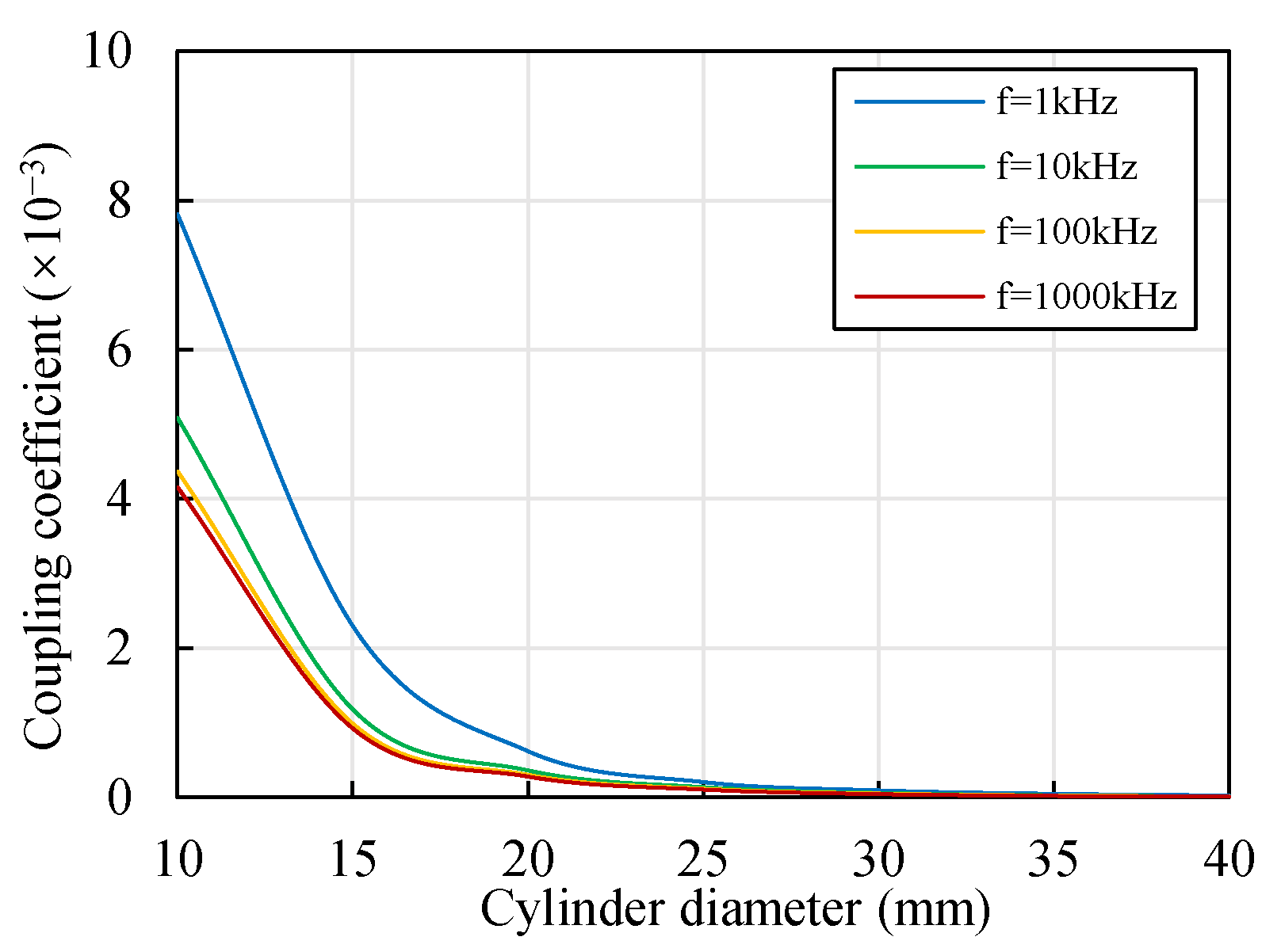
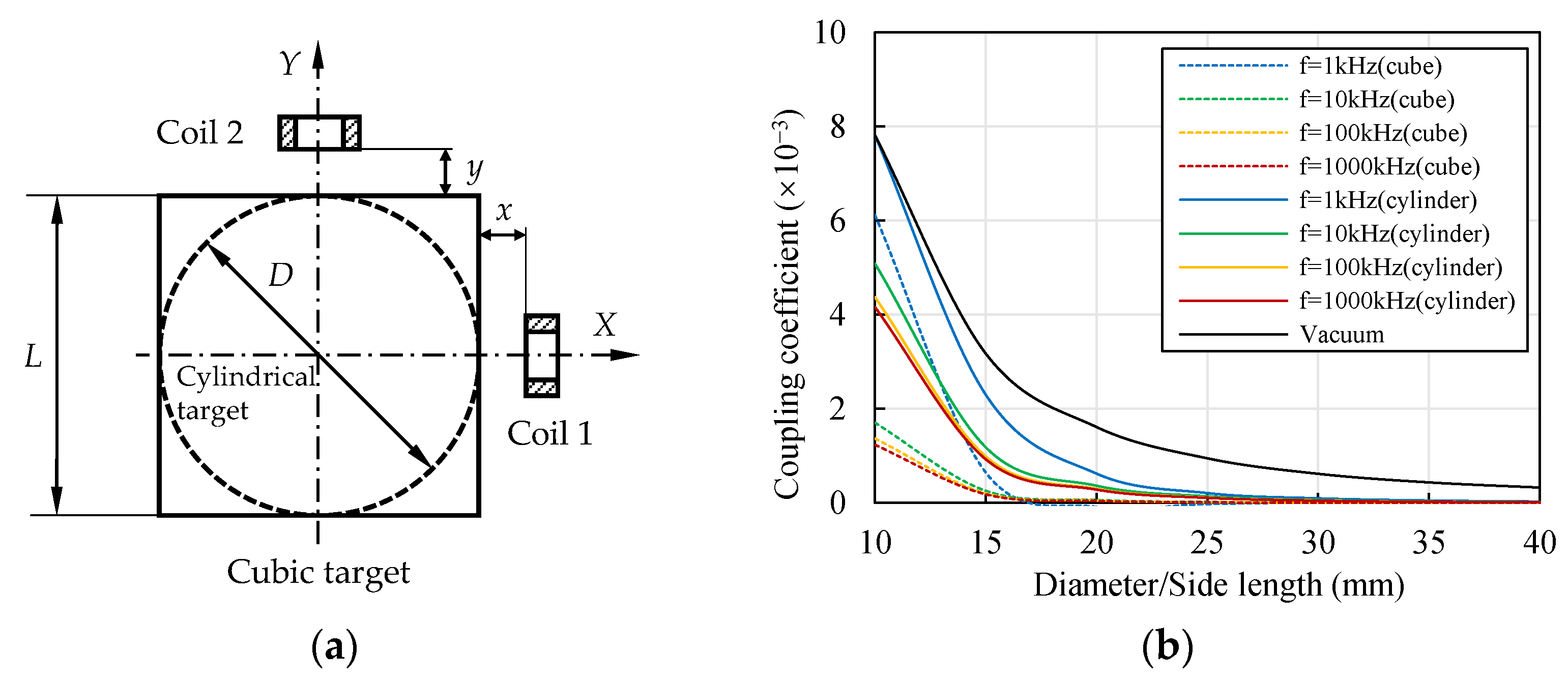
3.4. Influence of Cylinder Diameter on the Coupling Effect
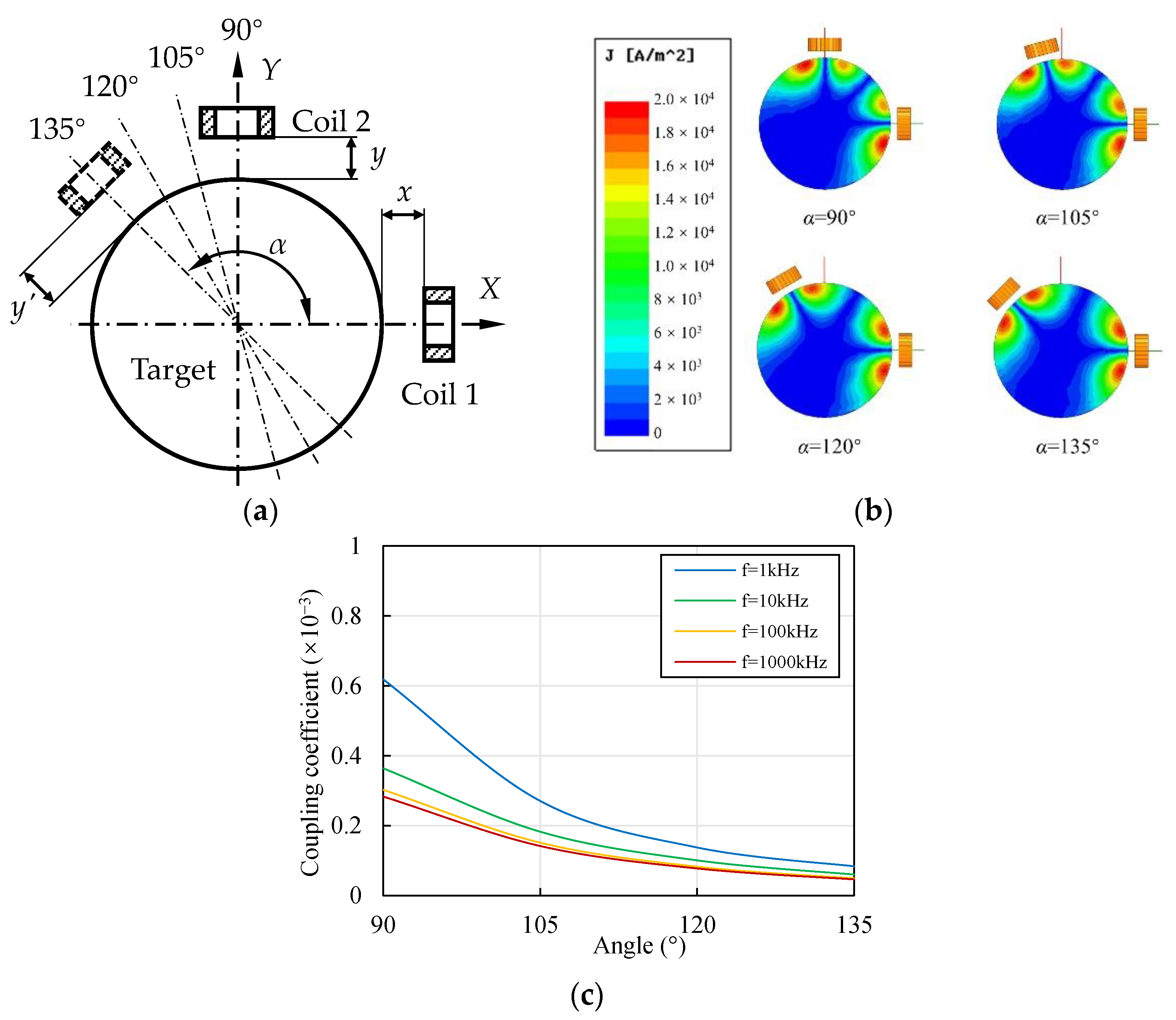
3.5. Influence of Coil Axis Angle on the Coupling Effect
3.6. Influence of Material on Coupling Effect
4. Experiments and Discussions
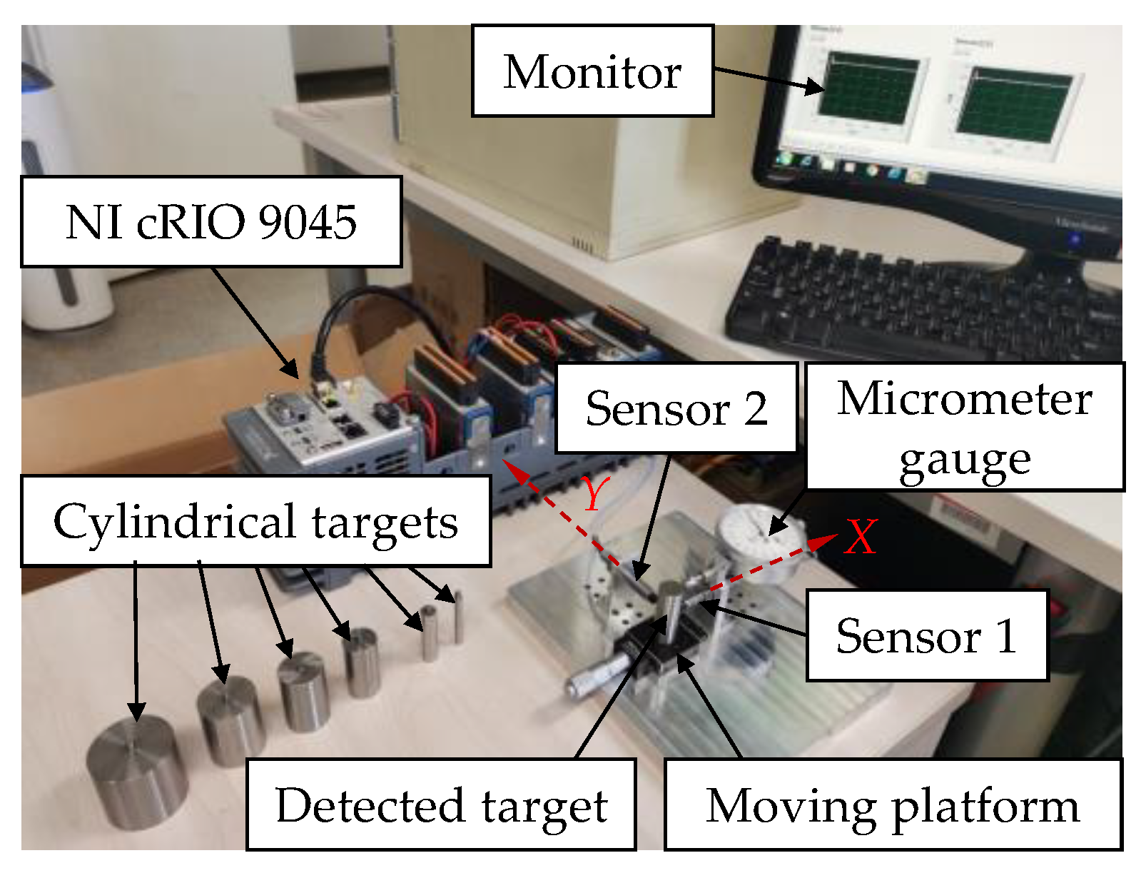
4.1. Experiment Design and Instruments
4.2. Calibration of Eddy Current Sensors on Cylindrical Targets
4.3. Influence of Coupling Effect on Measured Output Signal
4.4. Compensation Method
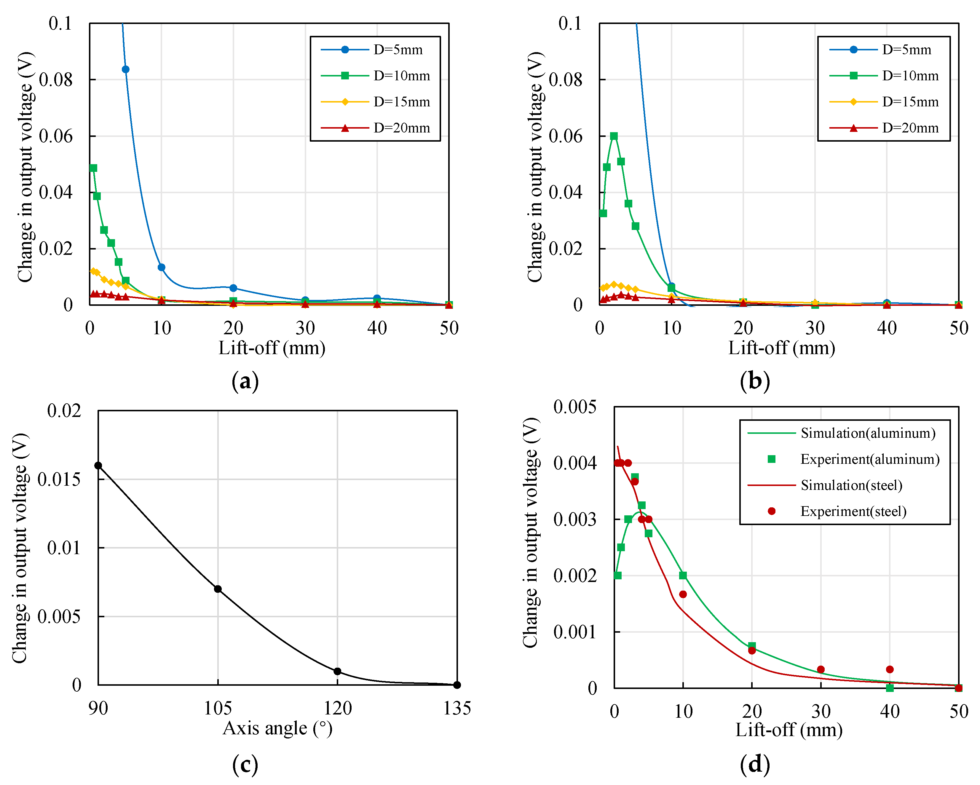
- The maximum value of |ΔU1| is evaluated. The application scenario is certain; thus, parameters including the material and diameter of the target, the diameter, axis angle, and excitation frequency of the ECS coils are constant. The lift-off values of sensors are typically variable. Therefore, with the change in lift-off y in a certain range, where y = +∞ if sensor 2 is OFF, the variations in |ΔU1| should be estimated. Two methods, either by experiments or FEM simulation, can be adopted. The values of |ΔU1| could be measured at full scale, and the maximum value of |ΔU1|, marked as |ΔU1|max, can be obtained from the experimental results, as shown in Figure 13a,b. The values of |ΔU1| can also be calculated by obtaining the values of the coupling coefficient in a 3D FEM simulation model, measuring the value of |ΔU1| at one single point, and transforming the values of coupling coefficient to |ΔU1| at full scale. Then, the value of |ΔU1|max can be obtained from the results, as shown in Figure 13d.
- 2.
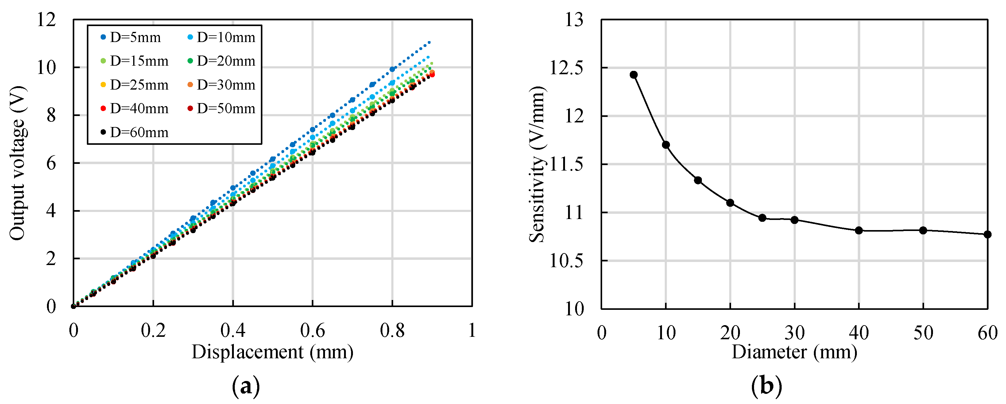
- |ΔU1|max is transformed to the maximum value of displacement error Emax. According to the calibration data shown in Figure 12a,b, the maximum value of displacement error, Emax, can be obtained by dividing |ΔU1|max by the sensitivity of the ECS.
- 3.
- Emax is contrasted with the value of the maximum permitted displacement error E. In the measurement of displacement, the maximum permitted error is always given. The permitted error is typically within 1 μm, for example, for a rotor with a bearing clearance of 10 μm, where the corresponding eccentricity error is 0.1. If the maximum value of displacement error Emax exceeds the permitted value E, compensation should be employed.
- (1)
- The output voltages of the eddy current sensors are collected. Signal processing circuits are necessary, which can provide excitation voltages to the coils, transform the values of impedance to voltages, and process the signals by amplifiers and filters. Then, the output voltage U1 of sensor 1 along the X direction is collected by an ADC module. The resolution of displacement measurement depends on the resolution of the ADC module; therefore, an ADC module with at least 12-bit resolution is recommended.
- (2)
- A compensation voltage is added to the original output voltage. The value of U1 contains the coupling interference of sensor 2 along the Y direction, which results in a decrease in voltage by |ΔU1|; therefore, the value of |ΔU1| should be compensated to U1. The value of |ΔU1| depends on the lift-off value y of sensor 2. Typically, y is transformed to |ΔU1| by a |ΔU1|–y function based on polynomial fitting, which is subsequently discussed in detail. The value of y can be obtained directly by sensor 2 if the lift-off is within the measurement range. Otherwise, y should be measured by other methods. The output voltage with compensation is U1c, where U1c = U1 + |ΔU1|.
- (3)
- The output voltage with compensation U1c is transformed to the displacement xc. The value of the displacement can be calculated based on the value of output voltage and the sensitivity obtained in Figure 12.
4.5. Motion Tracks of a Cylindrical Target with and without Compensation
5. Conclusions
- (1)
- The simulation and experimental results agreed closely, proving that the lift-off, cylinder diameter, axis angle, material, and excitation frequency influenced the coupling effect between the sensors. The coupling coefficient decreased with the increase in the lift-off, cylinder diameter, and axis angle. For different materials, the coupling coefficient changed differently with frequency.
- (2)
- Coupling interference decreased the output voltage of an ECS. The necessity of compensation should be estimated by considering the permitted displacement error and the maximum error generated by coupling interference. If compensation is necessary, compensation voltage can be obtained by polynomial fitting.
- (3)
- The compensation method can be used to measure the absolute position of a rotor, and the effect was proven with a simulation model, showing that the error significantly decreased.
6. Patents
Author Contributions
Funding
Institutional Review Board Statement
Informed Consent Statement
Data Availability Statement
Acknowledgments
Conflicts of Interest
References
- Garcia-Martin, J.; Gomez-Gil, J.; Vazquez-Sanchez, E. Non-destructive techniques based on eddy current testing. Sensors 2011, 11, 2525–2565. [Google Scholar] [CrossRef] [PubMed]
- AbdAlla, A.N.; Faraj, M.A.; Samsuri, F.; Rifai, D.; Ali, K.; Al-Douri, Y. Challenges in improving the performance of eddy current testing: Review. Meas. Control. 2018, 52, 46–64. [Google Scholar] [CrossRef]
- Papaelias, M.; Roberts, C.; Davis, C.L. A review on non-destructive evaluation of rails: State-of-the-art and future development. Proc. Inst. Mech. Eng. Part F J. Rail Rapid Transit 2008, 222, 367–384. [Google Scholar] [CrossRef]
- Gao, P.; Wang, C.; Zhi, Y.; Li, Y. Defect classification using phase lag information of EC-GMR output. Nondestruct. Test. Eval. 2014, 29, 229–242. [Google Scholar] [CrossRef]
- Nabavi, M.R.; Nihtianov, S.N. Design Strategies for Eddy-Current Displacement Sensor Systems: Review and Recommendations. IEEE Sens. J. 2012, 12, 3346–3355. [Google Scholar] [CrossRef]
- Fleming, A.J. A review of nanometer resolution position sensors: Operation and performance. Sens. Actuators A Phys. 2013, 190, 106–126. [Google Scholar] [CrossRef]
- Fahmi, A.; Kashyzadeh, K.R.; Ghorbani, S. A comprehensive review on mechanical failures cause vibration in the gas turbine of combined cycle power plants. Eng. Fail. Anal. 2022, 134, 106094. [Google Scholar] [CrossRef]
- Lu, M.; Xie, Y.; Zhu, W.; Peyton, A.; Yin, W. Determination of the Magnetic Permeability, Electrical Conductivity, and Thickness of Ferrite Metallic Plates Using a Multifrequency Electromagnetic Sensing System. IEEE Trans. Ind. Inform. 2019, 15, 4111–4119. [Google Scholar] [CrossRef]
- Yin, W.; Peyton, A.J. Thickness measurement of non-magnetic plates using multi-frequency eddy current sensors. NDT E Int. 2007, 40, 43–48. [Google Scholar] [CrossRef]
- Rosado, L.S.; Gonzalez, J.C.; Santos, T.G.; Ramos, P.M.; Piedade, M. Geometric optimization of a differential planar eddy currents probe for non-destructive testing. Sens. Actuators A Phys. 2013, 197, 96–105. [Google Scholar] [CrossRef]
- Chen, G.L.; Zhang, W.M.; Zhang, Z.J.; Jin, X.; Pang, W.H. A new rosette-like eddy current array sensor with high sensitivity for fatigue defect around bolt hole in SHM. Ndt E Int. 2018, 94, 70–78. [Google Scholar] [CrossRef]
- She, S.B.; Liu, Y.Z.; Zhang, S.J.; Wen, Y.Z.; Zhou, Z.J.; Liu, X.K.; Sui, Z.H.; Ren, D.T.; Zhang, F.; He, Y.Z. Flexible Differential Butterfly-Shape Eddy Current Array Sensor for Defect Detection of Screw Thread. IEEE Sens. J. 2021, 21, 20764–20777. [Google Scholar] [CrossRef]
- Chen, T.; He, Y.; Du, J. A High-Sensitivity Flexible Eddy Current Array Sensor for Crack Monitoring of Welded Structures under Varying Environment. Sensors 2018, 18, 1780. [Google Scholar] [CrossRef] [PubMed]
- Zhang, H.Y.; Ma, L.Y.; Xie, F.Q. A method of steel ball surface quality inspection based on flexible arrayed eddy current sensor. Measurement 2019, 144, 192–202. [Google Scholar] [CrossRef]
- Lu, M.Y.; Meng, X.B.; Huang, R.C.; Chen, L.M.; Peyton, A.; Yin, W.L. Lift-off invariant inductance of steels in multi-frequency eddy-current testing. Ndt E Int. 2021, 121, 102458. [Google Scholar] [CrossRef]
- Ona, D.I.; Tian, G.Y.; Sutthaweekul, R.; Naqvi, S.M. Design and optimisation of mutual inductance based pulsed eddy current probe. Measurement 2019, 144, 402–409. [Google Scholar] [CrossRef]
- Wang, H.; Feng, Z. Ultrastable and highly sensitive eddy current displacement sensor using self-temperature compensation. Sens. Actuators A Phys. 2013, 203, 362–368. [Google Scholar] [CrossRef]
- Wang, H.; Ju, B.; Li, W.; Feng, Z. Ultrastable eddy current displacement sensor working in harsh temperature environments with comprehensive self-temperature compensation. Sens. Actuators A Phys. 2014, 211, 98–104. [Google Scholar] [CrossRef]
- Mizuno, T.; Enoki, S.; Asahina, T.; Suzuki, T.; Maeda, H.; Asahi, T.; Shinagawa, H. Output voltage characteristics of eddy current displacement sensor for various heat treatments of measuring objects. Trans. Inst. Electr. Eng. Jpn. A 2008, 128, 289–297. [Google Scholar] [CrossRef]
- Yating, Y.; Tuo, Y.; Pingan, D. A new eddy current displacement measuring instrument independent of sample electromagnetic properties. NDT E Int. 2012, 48, 16–22. [Google Scholar] [CrossRef]
- Li, Y.; Sheng, X.; Lian, M.; Wang, Y. Influence of tilt angle on eddy current displacement measurement. Nondestruct. Test. Eval. 2015, 31, 289–302. [Google Scholar] [CrossRef]
- Walton, J.F.; Heshmat, H.; Tomaszewski, M.J. Testing of a small turbocharger/turbojet sized simulator rotor supported on foil bearings. J. Eng. Gas. Turb. Power 2008, 130, 035001. [Google Scholar] [CrossRef]
- Mizumoto, H.; Arii, S.; Yabuta, Y.; Tazoe, Y. Vibration Control of a High-Speed Air-Bearing Spindle using an Active Aerodynamic Bearing. In Proceedings of the International Conference on Control, Automation and Systems (Iccas 2010), Goyang-si, Korea, 27–30 October 2010; pp. 2261–2264. [Google Scholar]
- Ding, T.; Chen, X. Eddy current sensor coil for measuring gaps between curved surfaces. J. Tsinghua Univ. Sci. Technol. 2006, 46, 180–183. [Google Scholar]
- Hu, Y.; Ding, T.; Wang, P. Characteristics of eddy current effects in curved flexible coils. J. Tsinghua Univ. Sci. Technol. 2013, 53, 1429–1433. [Google Scholar]
- Zhang, Y.-H.; Sun, H.-X.; Luo, F.-L. Suppression method of a probe-coil’s lift-off noise for the curved specimen with small curvature radius in eddy-current testing. Proc. CSEE 2009, 29, 126–132. [Google Scholar]
- Zhan, H.; Wang, L.; Wang, T.; Yu, J. The Influence and Compensation Method of Eccentricity for Cylindrical Specimens in Eddy Current Displacement Measurement. Sensors 2020, 20, 6608. [Google Scholar] [CrossRef]
- Sheng, X.J.; Li, Y.; Lian, M.; Xu, C.; Wang, Y.Q. Influence of Coupling Interference on Arrayed Eddy Current Displacement Measurement. Mater. Eval. 2016, 74, 1675–1683. [Google Scholar]
- Chiba, A. 18—Displacement sensors and sensorless operation. In Magnetic Bearings and Bearingless Drives; Chiba, A., Fukao, T., Ichikawa, O., Oshima, M., Takemoto, M., Dorrell, D.G., Eds.; Newnes: Oxford, UK, 2005; pp. 329–343. [Google Scholar]
- Pawlenka, T.; Skuta, J. Shaft Displacement Measurement Using Capacitive Sensors. In Proceedings of the 2021 22nd International Carpathian Control Conference (ICCC), Velké Karlovice, Czech Republic, 31 May–1 June 2021. [Google Scholar]
- Li, H.W.; Liang, Z.Q.; Pei, J.J.; Jiao, L.; Xie, L.J.; Wang, X.B. New Measurement Method for Spline Shaft Rolling Performance Evaluation using Laser Displacement Sensor. Chin. J. Mech. Eng. 2018, 31, 1–9. [Google Scholar] [CrossRef]
- Reda, K.; Yan, Y. Vibration Measurement of an Unbalanced Metallic Shaft Using Electrostatic Sensors. IEEE Trans. Instrum. Meas. 2019, 68, 1467–1476. [Google Scholar] [CrossRef]
- Liu, F.X.; Yang, Y.; Jiang, D.; Ruan, X.B.; Chen, X.L. Modeling and Optimization of Magnetically Coupled Resonant Wireless Power Transfer System With Varying Spatial Scales. IEEE Trans. Power Electron. 2017, 32, 3240–3250. [Google Scholar] [CrossRef]
- Raju, S.; Wu, R.X.; Chan, M.S.; Yue, C.P. Modeling of Mutual Coupling Between Planar Inductors in Wireless Power Applications. Ieee Trans. Power Electron. 2014, 29, 481–490. [Google Scholar] [CrossRef]
- Yating, Y.; Pingan, D. Two approaches to coil impedance calculation of eddy current sensor. Proc. Inst. Mech. Eng. Part C J. Mech. Eng. Sci. 2008, 222, 507–515. [Google Scholar] [CrossRef]
- Li, Y.M.; Wu, J.; Guo, Q. Electromagnetic Sensor for Detecting Wear Debris in Lubricating Oil. IEEE Trans. Instrum. Meas. 2020, 69, 2533–2541. [Google Scholar] [CrossRef]
- Yu, Y.T.; Du, P.G. Optimization of an eddy current sensor using finite element method. In Proceedings of the IEEE International Conference on Mechatronics and Automation, Harbin, China, 5–8 August 2007; pp. 3795–3800. [Google Scholar]
- Yu, Y.T.; Du, P.A.; Wang, Z.W. Study on the electromagnetic properties of eddy current sensor. In Proceedings of the 2005 IEEE International Conference on Mechatronics and Automations, Niagara Falls, ON, Canada, 29 July–1 August 2005; pp. 1970–1975. [Google Scholar]
- Welsby, S.D.; Hitz, T. True position measurement with eddy current technology. Sensors 1997, 14, 30–41. [Google Scholar]
- Cao, F.; Wang, S.R.; Wang, G.Q.; Li, Y.D. The dynamics simulation analysis on turbocharger turbine-shaft system. In Proceedings of the International Conference on Mechanics and Architectural Design (MAD), Suzhou, China, 14–15 May 2016; pp. 42–49. [Google Scholar]
- Jinwei, W.; Zheng, W.; Xiujuan, W.; Hong, H.; Li, Z.; Haiyun, P. Research on the connection technology of TiAl alloy turbine in diesel engine turbocharger. In Proceedings of the 2014 ISFMFE—6th International Symposium on Fluid Machinery and Fluid Engineering, Wuhan, China, 22–22 October 2014; pp. 1–3. [Google Scholar]
- Wang, W.; Li, X.; Zeng, Q.; Lou, F.; Lai, T.; Hou, Y. Stability analysis for fully hydrodynamic gas-lubricated protuberant foil bearings in high speed turbomachinery. J. Xi’an Jiaotong Univ. 2017, 51, 84–89. [Google Scholar]


| Material | σ (MS/m) | μr |
|---|---|---|
| Vacuum | 0 | 1 |
| Copper | 58 | 0.999991 |
| Aluminum | 38 | 1.000021 |
| Steel 1008 | 2 | referring to the B–H curve shown in Figure 3b |
Publisher’s Note: MDPI stays neutral with regard to jurisdictional claims in published maps and institutional affiliations. |
© 2022 by the authors. Licensee MDPI, Basel, Switzerland. This article is an open access article distributed under the terms and conditions of the Creative Commons Attribution (CC BY) license (https://creativecommons.org/licenses/by/4.0/).
Share and Cite
Zhang, W.; Bu, J.; Li, D.; Zhang, K.; Zhou, M. Coupling Interference between Eddy Current Sensors for the Radial Displacement Measurement of a Cylindrical Target. Sensors 2022, 22, 4375. https://doi.org/10.3390/s22124375
Zhang W, Bu J, Li D, Zhang K, Zhou M. Coupling Interference between Eddy Current Sensors for the Radial Displacement Measurement of a Cylindrical Target. Sensors. 2022; 22(12):4375. https://doi.org/10.3390/s22124375
Chicago/Turabian StyleZhang, Weifeng, Jianguo Bu, Dongjie Li, Ke Zhang, and Ming Zhou. 2022. "Coupling Interference between Eddy Current Sensors for the Radial Displacement Measurement of a Cylindrical Target" Sensors 22, no. 12: 4375. https://doi.org/10.3390/s22124375
APA StyleZhang, W., Bu, J., Li, D., Zhang, K., & Zhou, M. (2022). Coupling Interference between Eddy Current Sensors for the Radial Displacement Measurement of a Cylindrical Target. Sensors, 22(12), 4375. https://doi.org/10.3390/s22124375