
Deep Learning Approach to Impact Classification in Sensorized Panels Using Self-Attention


Abstract
:1. Introduction
2. Deep Learning for SHM
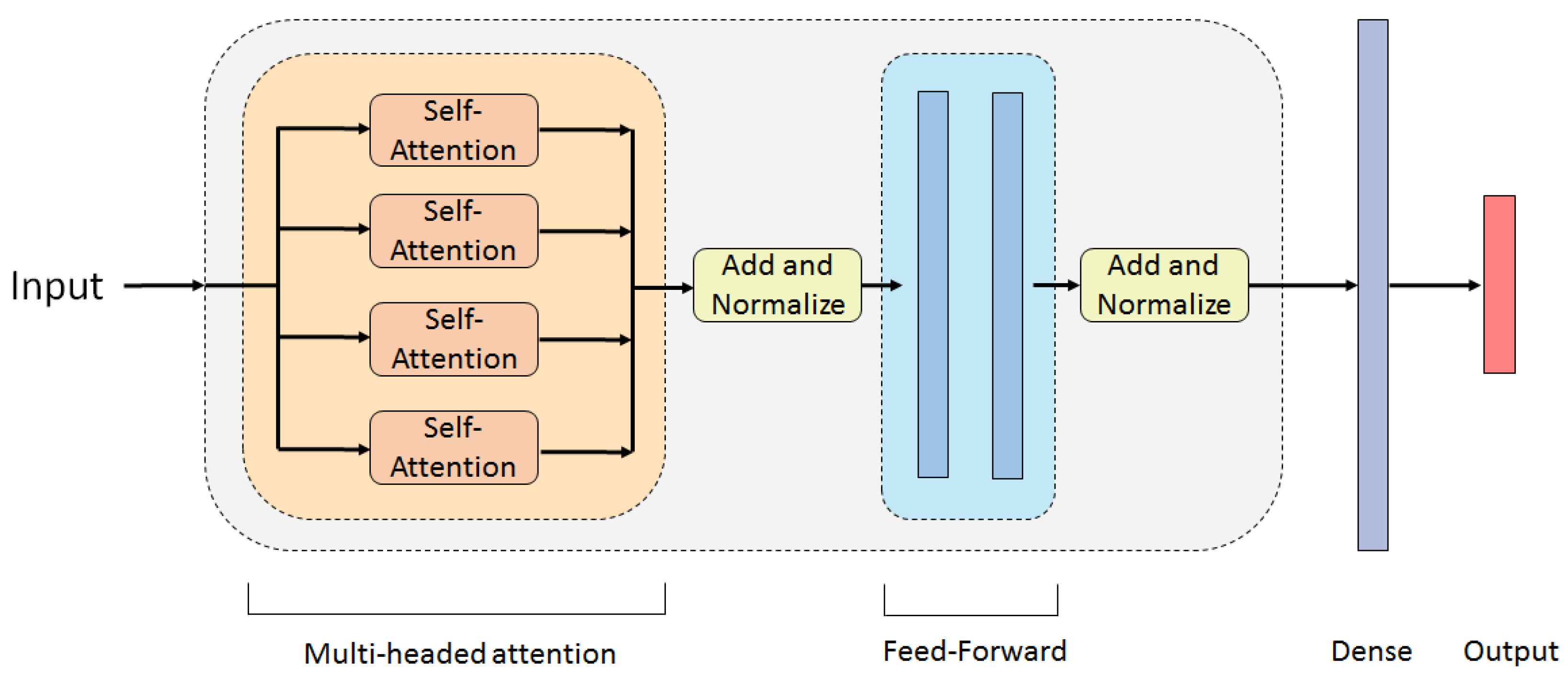
Transformer Model
- Embedding: Before the input vector is fed into the network, it is embedded. This is useful in text applications, where the inputs are whole numbers that correspond to the key values for words in a dictionary/vocabulary. The Embedding replaces each word/key value with a unique dense vector, through the use of unsupervised learning, or look-up tables. Similar words are mapped to similar dense vectors. The sequence of S number of words is converted into a matrix, where each row is a dense vector (embedding) of length , representing a word. Encoding the inputs this way allows for a more consistent backpropagation during network learning.
- Positional Encoding: The positional encoding creates vectors of the positions of each word in the input sequence, via sine and cosine functions. After the positional vector is created, it is added to the word embedding. This ensures that the Transformer not only has information about the word, but also its position in the sequence, which allows for parallelization. The input matrix, containing embeddings with positional encoding, is fed to the first encoder.
- Self-Attention: The heart of the Transformer model, the Self-Attention sub-layer, weighs the relationships between each embedding in the input sequence and all other embeddings in that sequence. It selectively focuses the attention of the Transformer towards the embeddings that have the highest effect on the model performance. In order to do so, the input matrix is passed through three linear transformations, to produce three different matrices:where Q, K and V are the query, key, and value matrices of column dimensions , , and , respectively, and is the input matrix. The transformation matrices, , and , are the learnable parameters for this part of the layer and are updated during backpropagation. The scaled dot-product attention is then calculated using the equation:where is a matrix of size , describing the relations between embeddings. As the queries, keys and values are calculated from the same input ( the previous layer) the Attention is called Self-Attention.
- Multi-Headed Attention: Passing the data through one Self-Attention sub-layer will extract some data dependencies. In order to boost performance and capture a larger number of relations from a sequence, N number of Self-Attention sub-layers (heads) can be stacked in parallel to create a Multi-Headed Attention sub-layer. Q, K and V matrices are created for each head independently, using learned linear projection weight matrices. The column dimensions of the query, key, and value for each head are taken to be the same, equal to . This creates different subspace representations of the query, key, and value for each Attention head, which then are fed into the scaled dot-product attention:where i denotes the head number, are the projection weight matrices for the i-th head, and is the attention matrix of the i-th head [36]. The separate query, key and value representations allow each head to derive different information from the same input data. At the output of all the parallel heads, the calculated attention matrices are concatenated, to form a matrix with the dimensions of the input matrix, . This new matrix is multiplied by a matrix of weights . This extracts global relations from the sequence data. It also gives one more weight matrix for the network to optimize and improve performance. Deeper analysis into Self and Multi-Headed Attention can be found in [37,38].
- Feed-Forward Network: The feed-forward network (FFN) sub-layer extracts features from the Multi-Headed Attention output with the intention of further summarizing the encoding process, thus its input dimension is . The output of the FFN is fed into the next encoder layer. This limits the last layer of the network to be equal to in order for the output dimensions to be the same as the input. This ensures the next encoder layer will be able to read and manipulate the output from the previous one. In the original Transformer architecture, a two-layer network, with a ReLU activation, is used [28].
- Add and Norm: This operation consists of first applying a residual skip connection [39] around each of the encoder sub-layers, namely adding the input of the sub-layer to its output. This is followed by a layer normalization operation [40]. The Add and Norm is applied after the Multi-Headed Attention and the Feed-forward network sub-layers.
3. Research Methodology
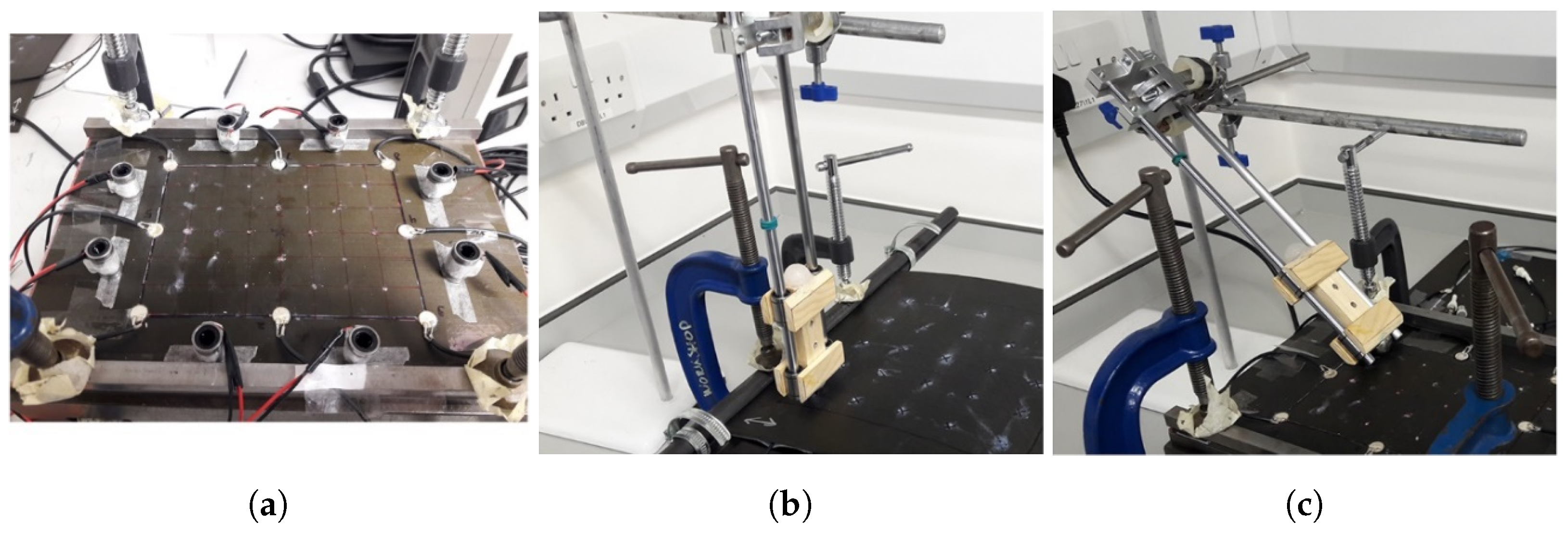
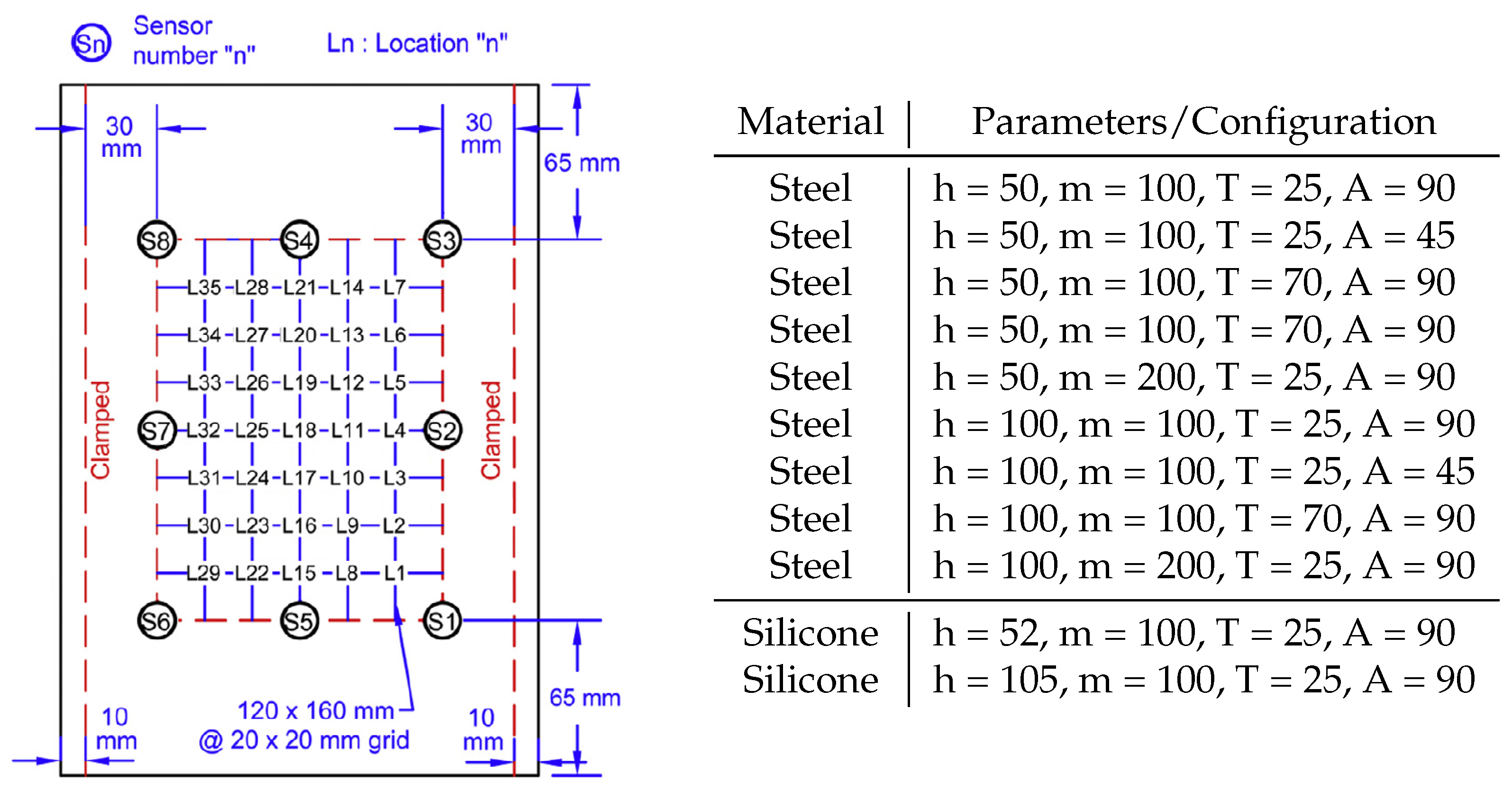
3.1. Experimental Data
- Safe: drop height-50 cm, mass-100 g/drop height-52 cm, mass-100 g;
- Warning: drop height-100 cm, mass-100 g/drop height-50 cm, mass-200 g/drop height-105 cm, mass-100 g;
- Danger: drop height-100 cm, mass-200 g.
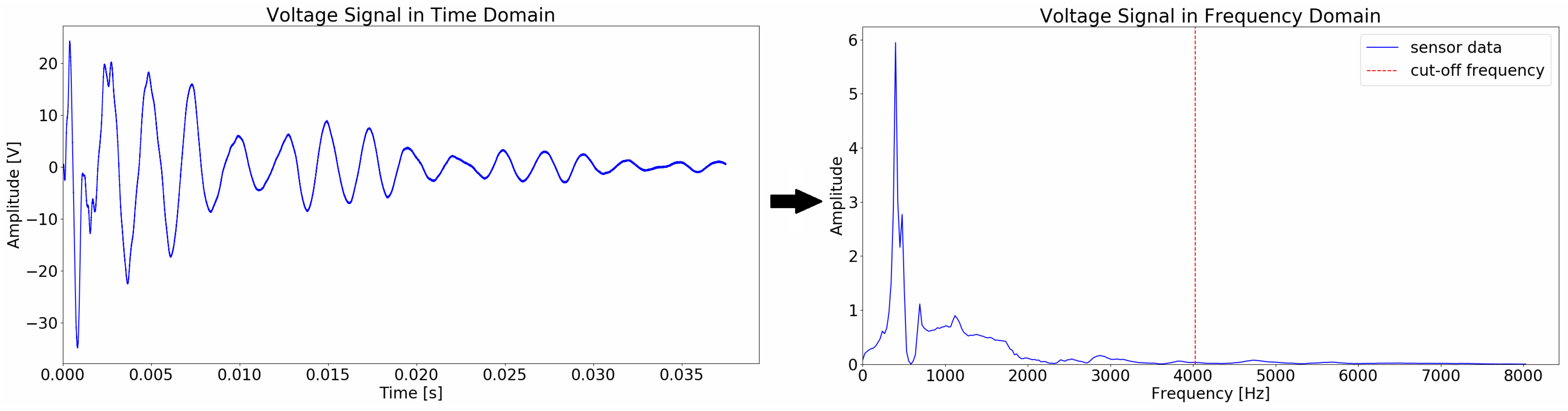
3.2. Data Transformation
4. Network Results and Performance
4.1. Impact Classification
4.1.1. Transformer
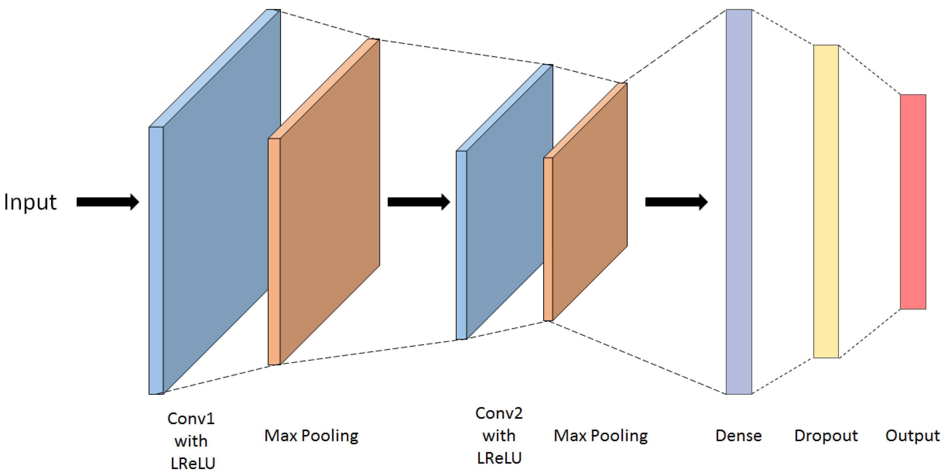
4.1.2. CNN
4.2. Angled Impact Dependency Investigation
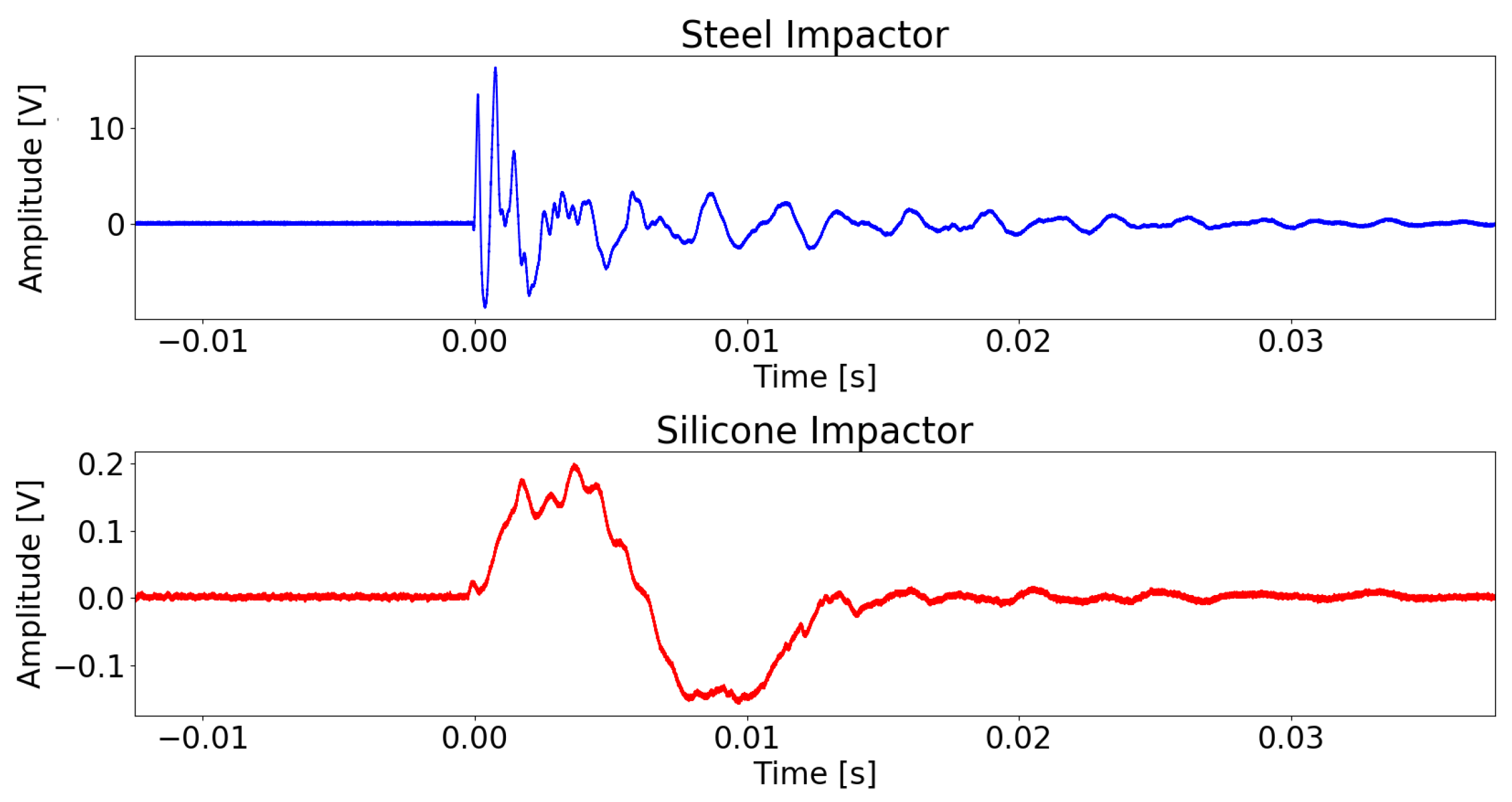
4.3. Silicone Impactor Dependency Investigation
5. Discussion and Comparison
5.1. Model Accuracy
5.2. Scalability
5.3. Training Time
5.4. Computational Demand
6. Conclusions
- Both the Transformer and CNN models are able to achieve 100% accuracy on impact energy classification, given steel impact signals.
- Both the Transformer and CNN were able to achieve highest accuracy with as little as 378 samples on steel data impactors. The further decrease in training samples deteriorated the Transformer’s performance on classifying and labels.
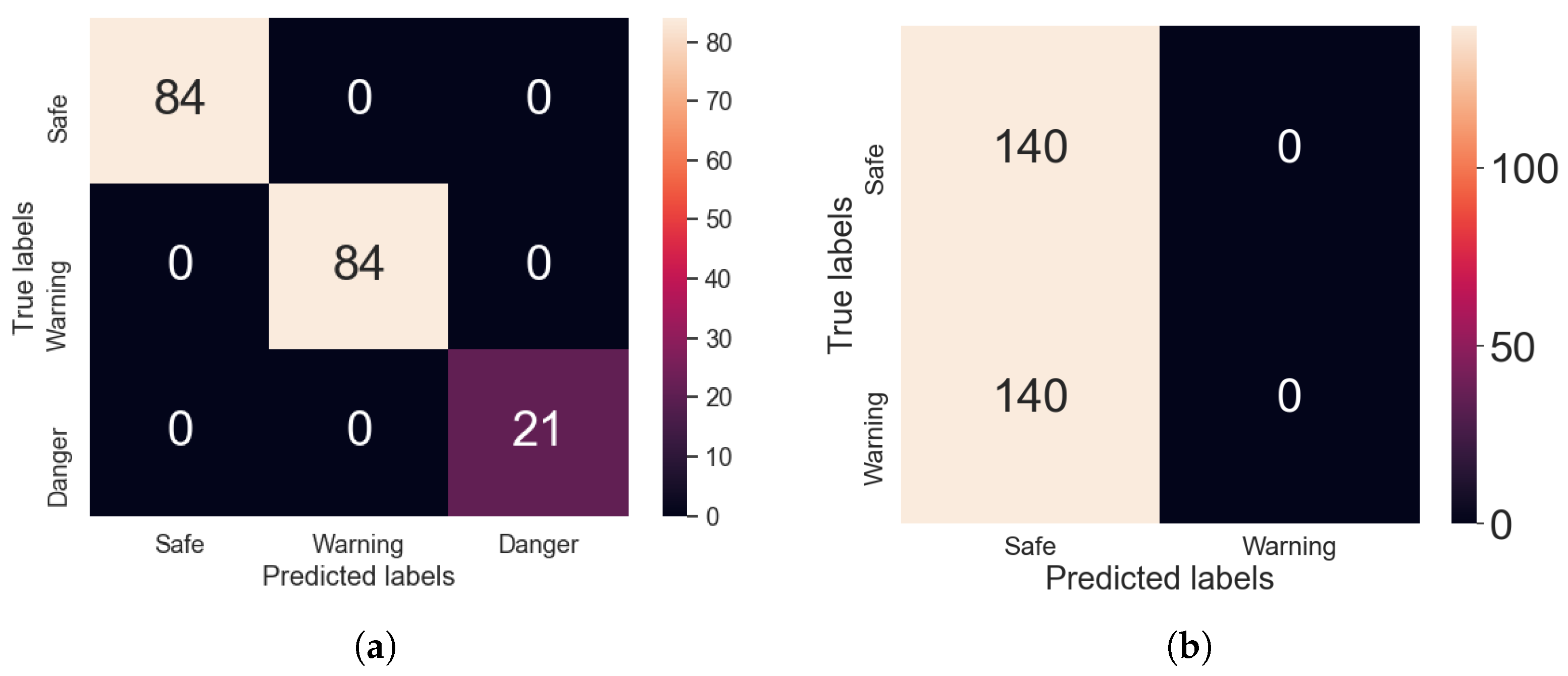
- The Transformer shows non-satisfactory up-scalability on new data sets. It is not able to accurately classify signals that are outside of the parameter distribution of its training set. The CNN equally struggles to predict data that lies outside its training samples.
- The Transformer is able to achieve pristine accuracy for any case when the training and testing data have the same distributions. The CNN equally achieves perfect prediction accuracy, when examples of the data it needs to predict have been present during its training. The two models are comparable on feature extraction and data generalization.
- The Transformer’s training time is approximately the same as that of the CNN, and it is much faster than the time required for NDT, making it a time-effective impact classification method.
- The Transformer, compared to CNN, requires much less computational power to train and run predictions. This makes it more flexible to be trained or executed on machines with less computational power, cutting costs from computational load.
- The Transformer requires 12% less memory space to be stored. This makes it more fit for aircraft applications where it would be implemented on-board, as aircraft free on-board memory is scarce. Even if not implemented on-board, the network saves memory space, cutting down costs.
Author Contributions
Funding
Data Availability Statement
Acknowledgments
Conflicts of Interest
Appendix A
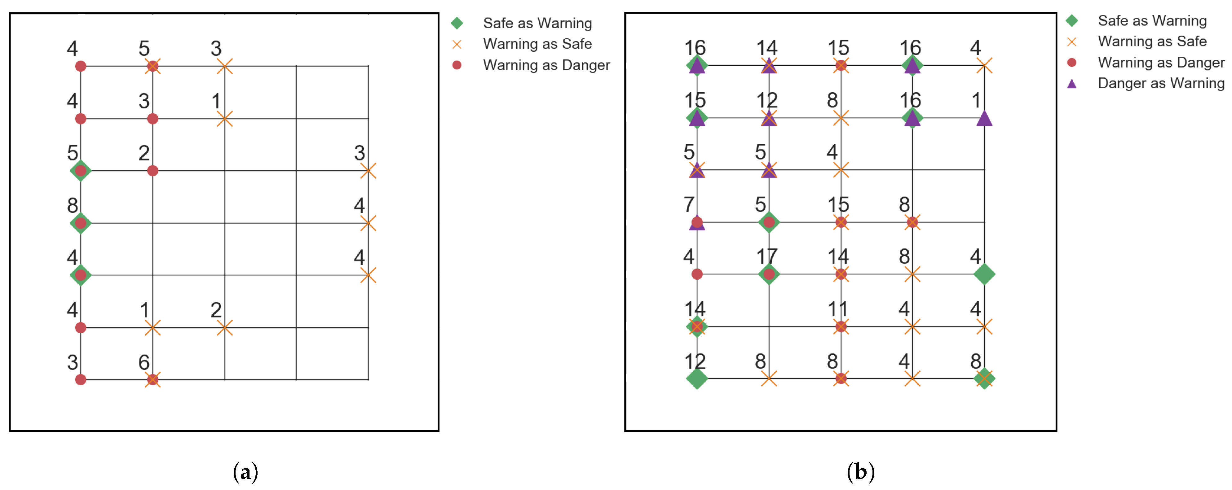
Appendix A.1. Transformer/CNN Validation Confusion Matrices
Appendix B
Appendix B.1. Model Comparison Table

| Transformer | CNN | |
|---|---|---|
| train: steel + steel (85%) test: steel + steel (15%) | 1 | 1 |
| train: steel + steel (85%) test: silicone | 0.333 | 0.333 |
| train: steel (85%) test: steel | 0.333 | 0.333 |
| train: steel + steel + silicone (85%) test: steel + steel + silicone (15%) | 1 | 1 |
| Transformer | CNN | |
|---|---|---|
| Training Time [s] | 54.4 | 48.3 |
| Storage Memory [KB] | 445 | 506 |
| Training Memory Usage [GB] | 1.2 | 1.9 |
| Memory Usage per Prediction [KB] | 11.9 | 15.3 |
References
- Soutis, C. Fibre reinforced composites in aircraft construction. Prog. Aerosp. Sci. 2005, 41, 143–151. [Google Scholar] [CrossRef]
- Slayton, R.; Spinardi, G. Radical innovation in scaling up: Boeing’s Dreamliner and the challenge of socio-technical transitions. Technovation 2016, 47, 47–58. [Google Scholar] [CrossRef]
- Halpin, J.C. Primer on Composite Materials Analysis, 2nd ed.; Revised; CRC Press: Boca Raton, FL, USA, 1992. [Google Scholar]
- Aliabadi, M.; Khodaei, Z. Structural Health Monitoring for Advanced Composite Structures; World Scientific Publishing: Singapore, 2017. [Google Scholar] [CrossRef]
- Petit, S.; Bouvet, C.; Bergerot, A.; Barrau, J.j. Impact and compression after impact experimental study of a composite laminate with a cork thermal shield. Compos. Sci. Technol. 2007, 67, 3286–3299. [Google Scholar] [CrossRef] [Green Version]
- Park, G.; Sohn, H.; Farrar, C.R.; Inman, D.J. Overview of Piezoelectric Impedance-Based Health Monitoring and Path Forward. Shock Vib. Dig. 2003, 35, 451–463. [Google Scholar] [CrossRef] [Green Version]
- Ostachowicz, W.; Güemes, A. New Trends in Structural Health Monitoring; CISM International Centre for Mechanical Sciences: Courses and Lectures; Springer: London, UK, 2013; Volume 542. [Google Scholar]
- Na, S.; Lee, H.K. Neural network approach for damaged area location prediction of a composite plate using electromechanical impedance technique. Compos. Sci. Technol. 2013, 88, 62–68. [Google Scholar] [CrossRef]
- Farrar, C.R.; Worden, K. Structural Health Monitoring: A Machine Learning Perspective, 1st ed.; Wiley: New York, NY, USA, 2012. [Google Scholar]
- Kessler, S.S.; Spearing, S.M.; Soutis, C. Damage detection in composite materials using Lamb wave methods. Smart Mater. Struct. 2002, 11, 269–278. [Google Scholar] [CrossRef] [Green Version]
- Seno, A.H.; Khodaei, Z.S.; Aliabadi, M.H.F. Passive sensing method for impact localisation in composite plates under simulated environmental and operational conditions. Mech. Syst. Signal Process. 2019, 129, 20–36. [Google Scholar] [CrossRef]
- Nayfeh, A.H.; Anderson, M.J. Wave Propagation in Layered Anisotropic Media with Applications to Composites. J. Acoust. Soc. Am. 2000, 108, 471–472. [Google Scholar] [CrossRef]
- Lamb, H. On Waves in an Elastic Plate; Royal Society: London, UK, 1917. [Google Scholar]
- Worlton, D.C. Experimental Confirmation of Lamb Waves at Megacycle Frequencies. J. Appl. Phys. 1961, 32, 967–971. [Google Scholar] [CrossRef]
- Rose, J.L. A Baseline and Vision of Ultrasonic Guided Wave Inspection Potential. J. Press. Vessel. Technol. 2002, 124, 273–282. [Google Scholar] [CrossRef]
- Viktorov, I.A. Rayleigh and Lamb Waves: Physical Theory and Applications; Plenum Press: New York, NY, USA, 1967. [Google Scholar]
- Su, Z.; Ye, L.; Lu, Y. Guided Lamb waves for identification of damage in composite structures: A review. J. Sound Vib. 2006, 295, 753–780. [Google Scholar] [CrossRef]
- Jia, F.; Lei, Y.; Lin, J.; Zhou, X.; Lu, N. Deep neural networks: A promising tool for fault characteristic mining and intelligent diagnosis of rotating machinery with massive data. Mech. Syst. Signal Process. 2016, 73, 303–315. [Google Scholar] [CrossRef]
- Seno, A.H.; Aliabadi, M.F. Impact Localisation in Composite Plates of Different Stiffness Impactors under Simulated Environmental and Operational Conditions. Sensors 2019, 19, 3659. [Google Scholar] [CrossRef] [PubMed] [Green Version]
- Seno, A.H.; Aliabadi, M.F. A novel method for impact force estimation in composite plates under simulated environmental and operational conditions. Smart Mater. Struct. 2020, 29, 115029. [Google Scholar] [CrossRef]
- Seno, A.H.; Aliabadi, M.F. Uncertainty quantification for impact location and force estimation in composite structures. Struct. Health Monit. 2021, 21, 1061–1075. [Google Scholar] [CrossRef]
- Lin, Y.z.; Nie, Z.h.; Ma, H.w. Structural Damage Detection with Automatic Feature-Extraction through Deep Learning. Comput.-Aided Civ. Infrastruct. Eng. 2017, 32, 1025–1046. [Google Scholar] [CrossRef]
- Saxena, A.; Saad, A. Evolving an artificial neural network classifier for condition monitoring of rotating mechanical systems. Appl. Soft Comput. 2007, 7, 441–454. [Google Scholar] [CrossRef]
- Selva, P.; Cherrier, O.; Budinger, V.; Lachaud, F.; Morlier, J. Smart monitoring of aeronautical composites plates based on electromechanical impedance measurements and artificial neural networks. Eng. Struct. 2013, 56, 794–804. [Google Scholar] [CrossRef] [Green Version]
- Abdeljaber, O.; Avci, O.; Kiranyaz, S.; Gabbouj, M.; Inman, D.J. Real-time vibration-based structural damage detection using one-dimensional convolutional neural networks. J. Sound Vib. 2017, 388, 154–170. [Google Scholar] [CrossRef]
- Oliveira, M.A.D.; Monteiro, A.V.; Filho, J.V. A New Structural Health Monitoring Strategy Based on PZT Sensors and Convolutional Neural Network. Sensors 2018, 18, 2955. [Google Scholar] [CrossRef] [Green Version]
- Guo, T.; Wu, L.; Wang, C.; Xu, Z. Damage detection in a novel deep-learning framework: A robust method for feature extraction. Struct. Health Monit. 2020, 19, 424–442. [Google Scholar] [CrossRef]
- Vaswani, A.; Shazeer, N.; Parmar, N.; Uszkoreit, J.; Jones, L.; Gomez, A.N.; Kaiser, L.; Polosukhin, I. Attention Is All You Need. arXiv 2017, arXiv:1706.03762. [Google Scholar] [CrossRef]
- Radford, A.; Narasimhan, K.; Salimans, T.; Sutskever, I. Improving Language Understanding by Generative Pre-Training; Technical Report; OpenAI: San Francisco, CA, USA, 2018. [Google Scholar]
- Devlin, J.; Chang, M.W.; Lee, K.; Toutanova, K. BERT: Pre-Training of Deep Bidirectional Transformers for Language Understanding. arXiv 2018, arXiv:1810.04805. [Google Scholar] [CrossRef]
- Popel, M.; Bojar, O. Training Tips for the Transformer Model. Prague Bull. Math. Linguist. 2018, 110, 43–70. [Google Scholar] [CrossRef] [Green Version]
- Dosovitskiy, A.; Beyer, L.; Kolesnikov, A.; Weissenborn, D.; Zhai, X.; Unterthiner, T.; Dehghani, M.; Minderer, M.; Heigold, G.; Gelly, S.; et al. An Image is Worth 16 × 16 Words: Transformers for Image Recognition at Scale. arXiv 2020, arXiv:2010.11929. [Google Scholar] [CrossRef]
- Schmidhuber, J. Deep learning in neural networks: An overview. Neural Netw. 2015, 61, 85–117. [Google Scholar] [CrossRef] [Green Version]
- Hochreiter, S.; Schmidhuber, J. Long Short-Term Memory. Neural Comput. 1997, 9, 1735–1780. [Google Scholar] [CrossRef]
- Sutskever, I.; Vinyals, O.; Le, Q.V. Sequence to Sequence Learning with Neural Networks. In Advances in Neural Information Processing Systems 27; Curran Associates Inc.: Red Hook, NY, USA, 2014; pp. 3104–3112. [Google Scholar]
- Cordonnier, J.B.; Loukas, A.; Jaggi, M. Multi-Head Attention: Collaborate Instead of Concatenate. arXiv 2020, arXiv:2006.16362. [Google Scholar] [CrossRef]
- Vig, J.; Belinkov, Y. Analyzing the Structure of Attention in a Transformer Language Model. arXiv 2019, arXiv:1906.04284. [Google Scholar] [CrossRef]
- Voita, E.; Talbot, D.; Moiseev, F.; Sennrich, R.; Titov, I. Analyzing Multi-Head Self-Attention: Specialized Heads Do the Heavy Lifting, the Rest Can Be Pruned. arXiv 2019, arXiv:1905.09418. [Google Scholar] [CrossRef]
- He, K.; Zhang, X.; Ren, S.; Sun, J. Deep Residual Learning for Image Recognition. In Proceedings of the 2016 IEEE Conference on Computer Vision and Pattern Recognition (CVPR), Las Vegas, NV, USA, 27–30 June 2016; pp. 770–778. [Google Scholar] [CrossRef] [Green Version]
- Ba, J.L.; Kiros, J.R.; Hinton, G.E. Layer Normalization. arXiv 2016, arXiv:1607.06450. [Google Scholar] [CrossRef]
- Lee-Thorp, J.; Ainslie, J.; Eckstein, I.; Ontanon, S. FNet: Mixing Tokens with Fourier Transforms. arXiv 2021, arXiv:2105.03824. [Google Scholar] [CrossRef]
- Srivastava, N.; Hinton, G.; Krizhevsky, A.; Sutskever, I.; Salakhutdinov, R. Dropout: A Simple Way to Prevent Neural Networks from Overfitting. J. Mach. Learn. Res. 2014, 15, 1929–1958. [Google Scholar]
- Keras. Available online: https://keras.io (accessed on 1 March 2022).

Publisher’s Note: MDPI stays neutral with regard to jurisdictional claims in published maps and institutional affiliations. |
© 2022 by the authors. Licensee MDPI, Basel, Switzerland. This article is an open access article distributed under the terms and conditions of the Creative Commons Attribution (CC BY) license (https://creativecommons.org/licenses/by/4.0/).
Share and Cite
Karmakov, S.; Aliabadi, M.H.F. Deep Learning Approach to Impact Classification in Sensorized Panels Using Self-Attention. Sensors 2022, 22, 4370. https://doi.org/10.3390/s22124370
Karmakov S, Aliabadi MHF. Deep Learning Approach to Impact Classification in Sensorized Panels Using Self-Attention. Sensors. 2022; 22(12):4370. https://doi.org/10.3390/s22124370
Chicago/Turabian StyleKarmakov, Stefan, and M. H. Ferri Aliabadi. 2022. "Deep Learning Approach to Impact Classification in Sensorized Panels Using Self-Attention" Sensors 22, no. 12: 4370. https://doi.org/10.3390/s22124370
APA StyleKarmakov, S., & Aliabadi, M. H. F. (2022). Deep Learning Approach to Impact Classification in Sensorized Panels Using Self-Attention. Sensors, 22(12), 4370. https://doi.org/10.3390/s22124370