
Multi-Swarm Algorithm for Extreme Learning Machine Optimization

 ,
,  ,
,  ,
,  ,
,  and
and
Abstract
:1. Introduction
2. Background
2.1. Extreme Learning Machine
2.2. Swarm Intelligence
2.3. ELM Tuning by Swarm Intelligence Meta-Heuristics
3. Proposed Hybrid Meta-Heuristics
3.1. Original Algorithms
3.1.1. The Original ABC Algorithm
3.1.2. The Original Firefly Algorithm
3.1.3. The Original SCA Method
3.2. Proposed Multi-Swarm Meta-Heuristics Algorithm
3.2.1. Motivation and Preliminaries
3.2.2. Overview of MS-AFS
- Chaotic and quasi-reflection-based learning (QRL) population initialization in order to establish boosting of the search by redirecting solutions towards more favorable parts of the domain;
- Efficient learning mechanism between swarms with the goal of combining weakness and strengths of different approaches more efficiently.
| Algorithm 1 Pseudo-code for chaotic and QRL population initialization |
|
| Algorithm 2 Search process of s1—ABC algorithm |
| Algorithm 3 Search process of s2—LLH between FA and SCA |
| Algorithm 4 High-level MS-AFS pseudo-code |
|
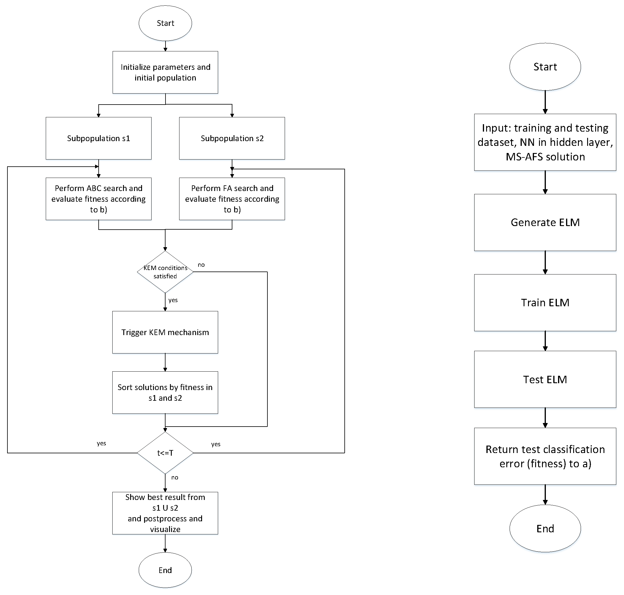
3.2.3. Computational Complexity, MS-AFS Solutions’ Encoding for ELM Tuning and Flow-Chart
4. Experiments
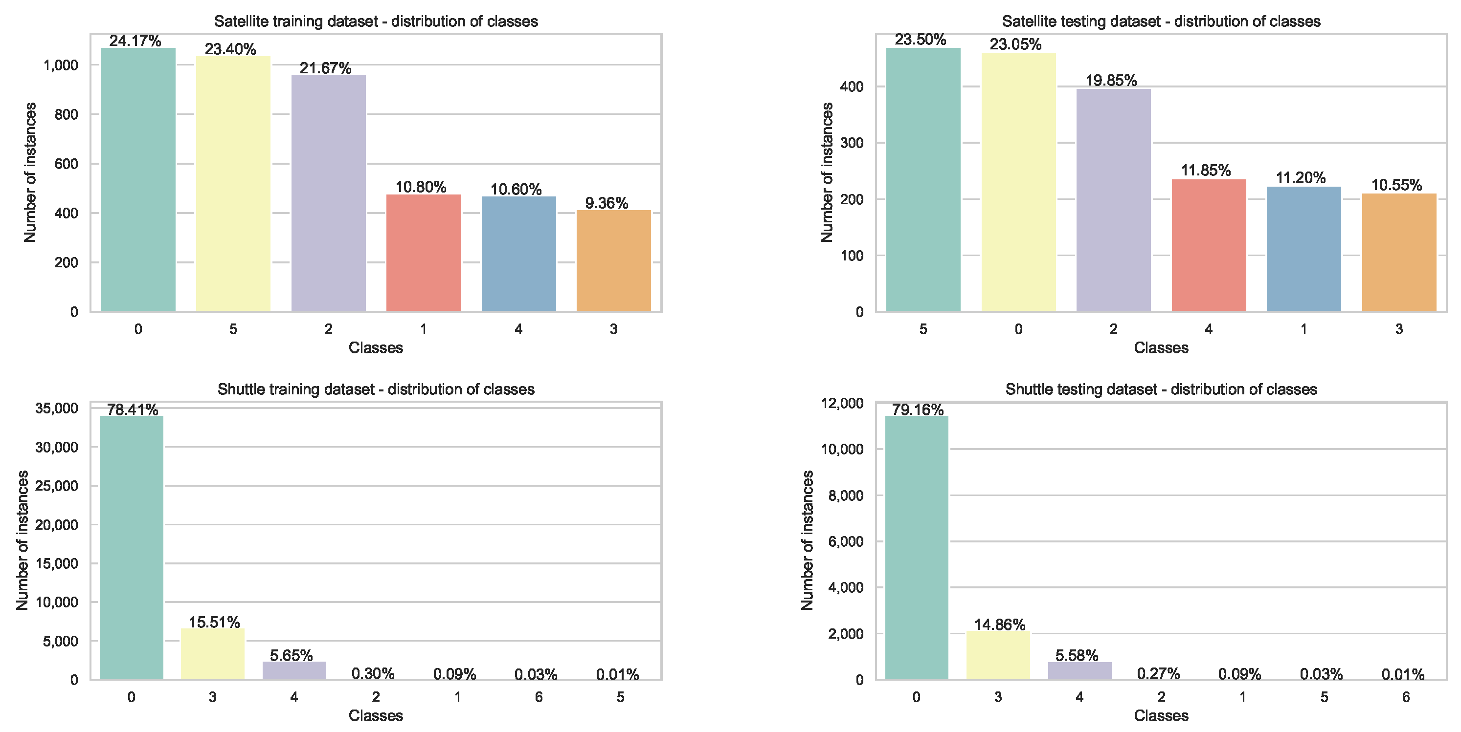
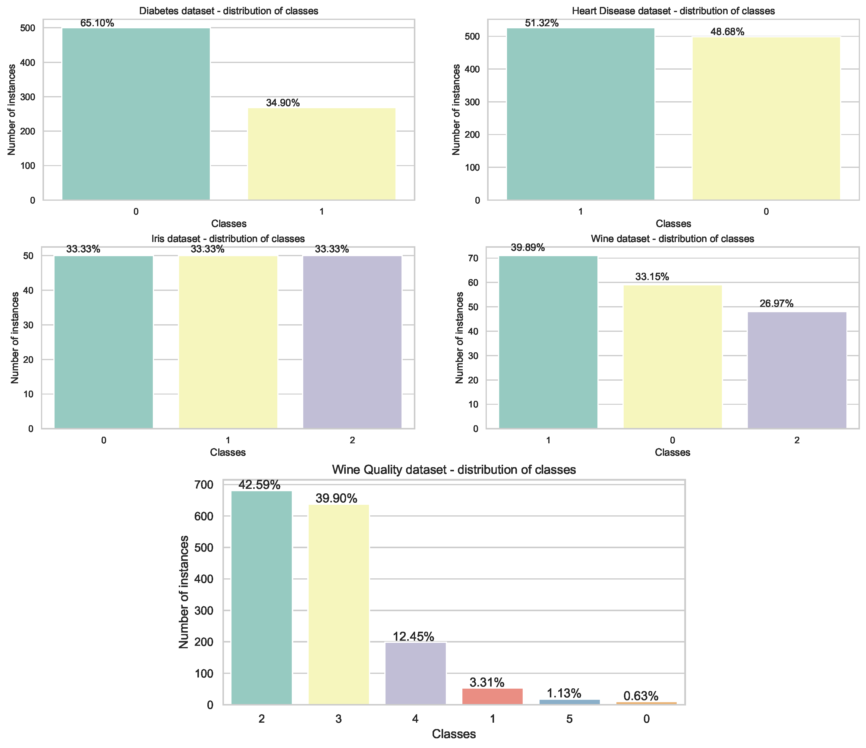
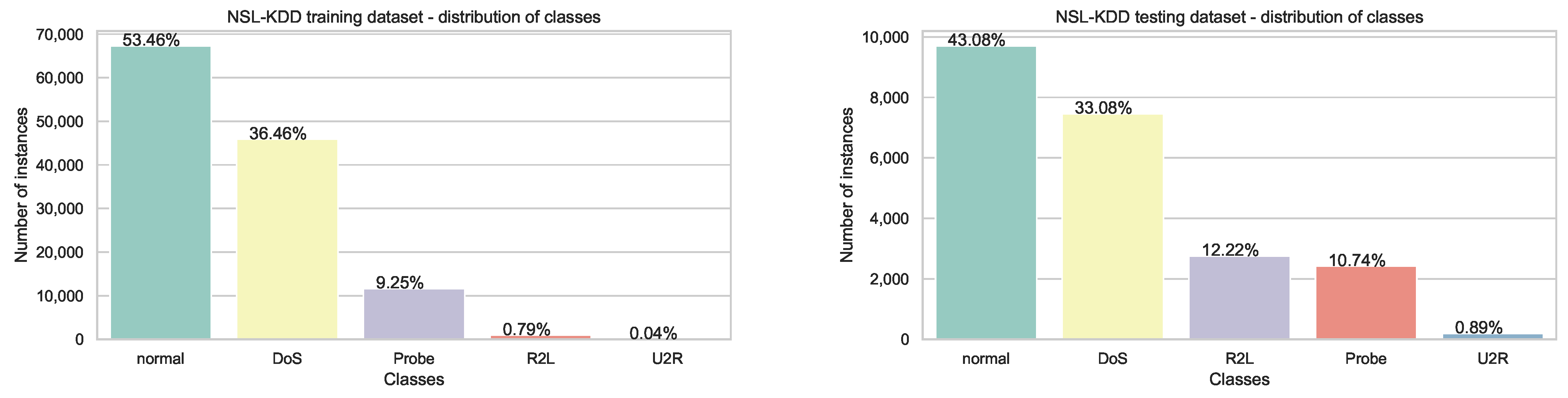
4.1. Datasets
4.2. Metrics
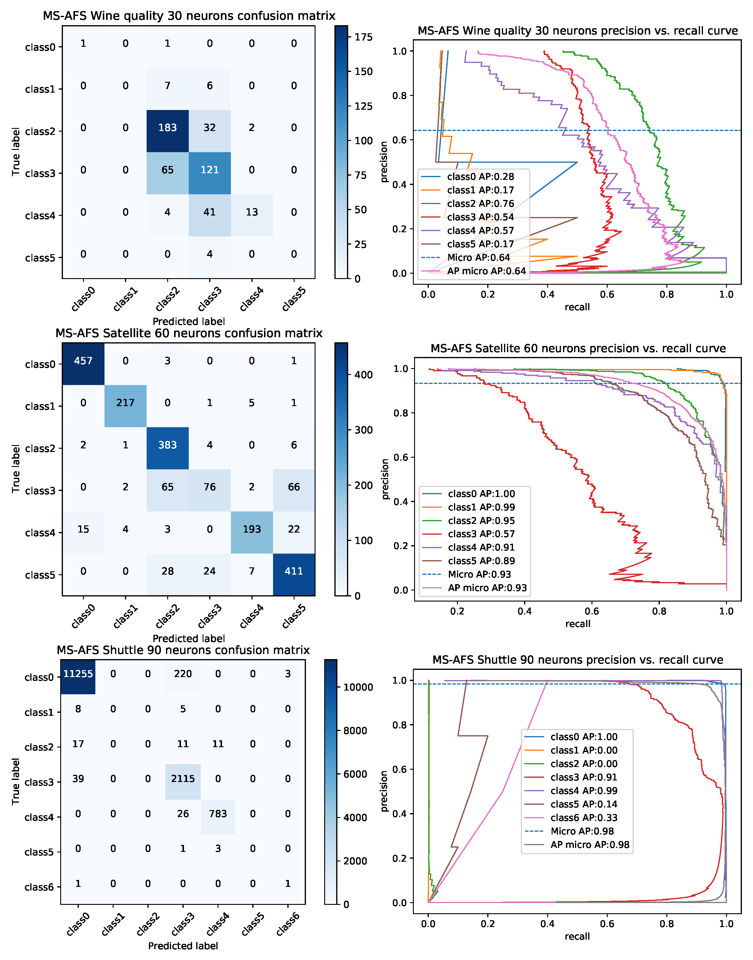
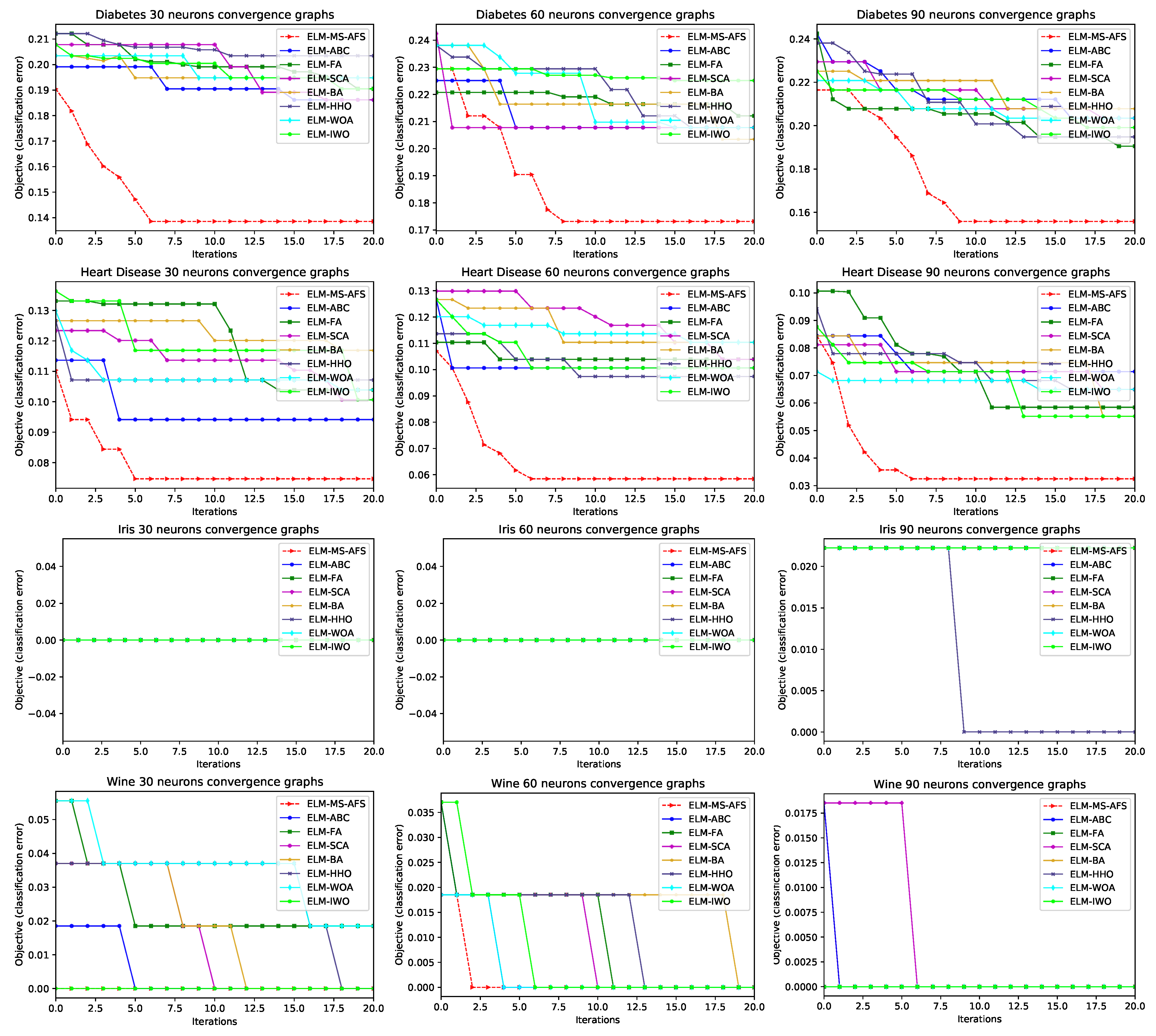
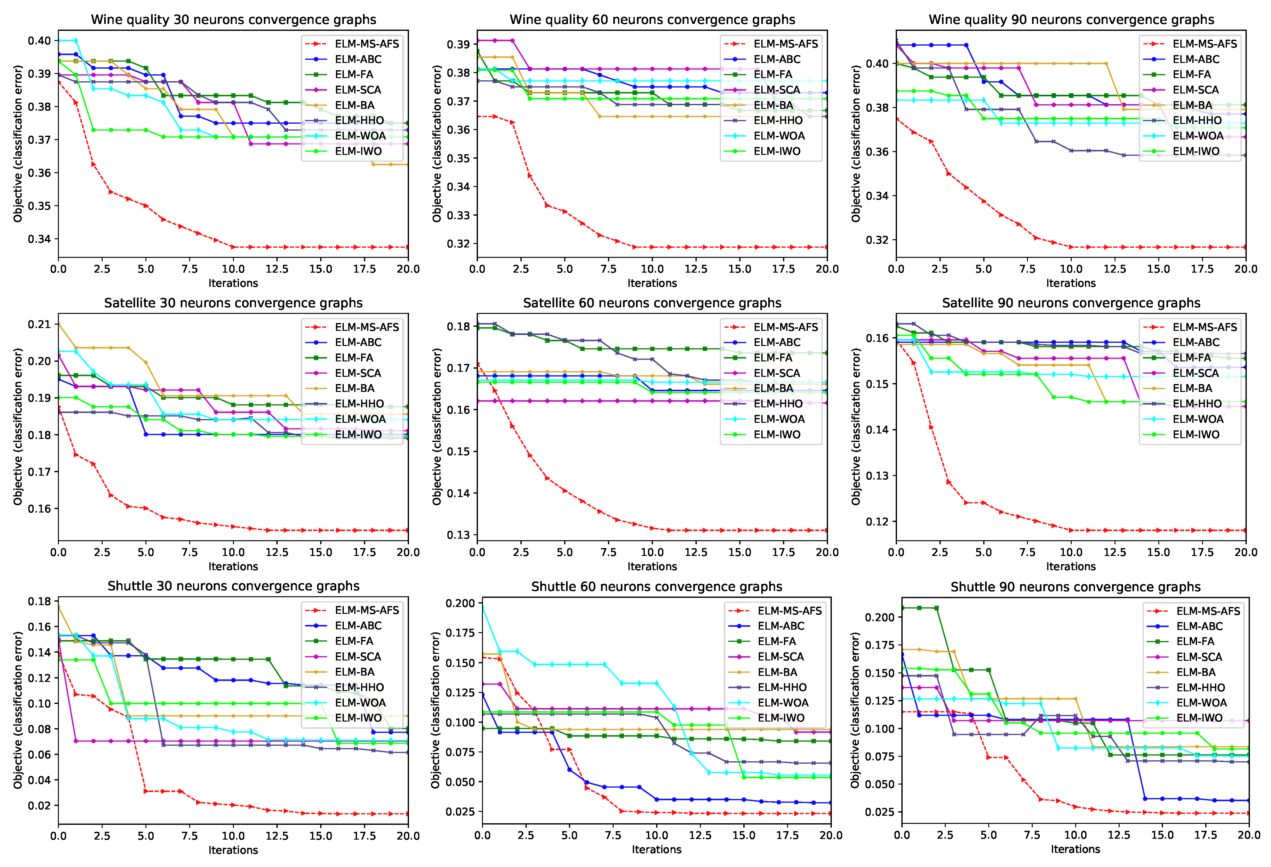
4.3. Experimental Results and Comparative Analysis with Other Cutting-Edge Meta-Heuristics
Statistical Tests
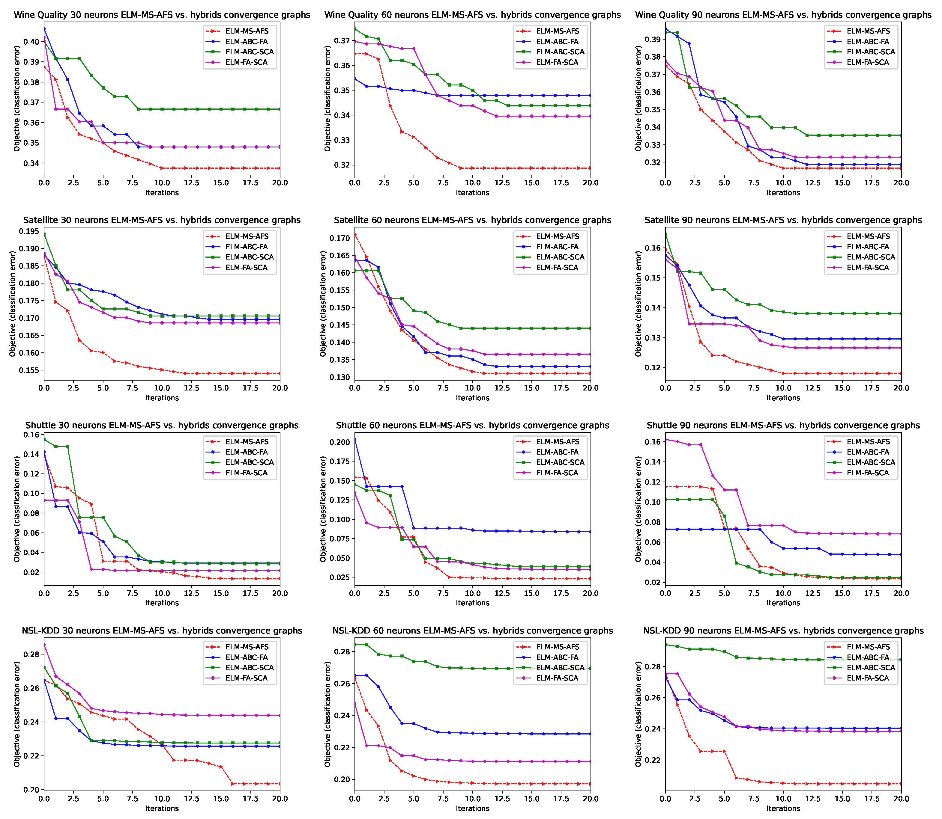
4.4. Hybridization by Pairs
5. Conclusions
Author Contributions
Funding
Institutional Review Board Statement
Informed Consent Statement
Data Availability Statement
Acknowledgments
Conflicts of Interest
References
- Huang, G.B.; Zhu, Q.Y.; Siew, C.K. Extreme learning machine: A new learning scheme of feedforward neural networks. In Proceedings of the 2004 IEEE International Joint Conference on Neural Networks (IEEE Cat. No.04CH37541), Budapest, Hungary, 25–29 July 2004; Volume 2, pp. 985–990. [Google Scholar] [CrossRef]
- Alshamiri, A.K.; Singh, A.; Surampudi, B.R. Two swarm intelligence approaches for tuning extreme learning machine. Int. J. Mach. Learn. Cybern. 2018, 9, 1271–1283. [Google Scholar] [CrossRef]
- Wang, J.; Lu, S.; Wang, S.; Zhang, Y.D. A review on extreme learning machine. Multimed. Tools Appl. 2021, 1–50. [Google Scholar] [CrossRef]
- Rong, H.J.; Ong, Y.S.; Tan, A.H.; Zhu, Z. A fast pruned-extreme learning machine for classification problem. Neurocomputing 2008, 72, 359–366. [Google Scholar] [CrossRef]
- Zhu, Q.Y.; Qin, A.; Suganthan, P.; Huang, G.B. Evolutionary extreme learning machine. Pattern Recognit. 2005, 38, 1759–1763. [Google Scholar] [CrossRef]
- Cao, J.; Lin, Z.; Huang, G.B. Self-adaptive evolutionary extreme learning machine. Neural Process. Lett. 2012, 36, 285–305. [Google Scholar] [CrossRef]
- Miche, Y.; Sorjamaa, A.; Bas, P.; Simula, O.; Jutten, C.; Lendasse, A. OP-ELM: Optimally pruned extreme learning machine. IEEE Trans. Neural Netw. 2009, 21, 158–162. [Google Scholar] [CrossRef]
- Huang, G.B.; Chen, L.; Siew, C.K. Universal approximation using incremental constructive feedforward networks with random hidden nodes. IEEE Trans. Neural Netw. 2006, 17, 879–892. [Google Scholar] [CrossRef] [Green Version]
- Serre, D. Matrices: Theory and Applications; Springer: Berlin/Heidelberg, Germany, 2002. [Google Scholar]
- Huang, G.B.; Zhu, Q.Y.; Siew, C.K. Extreme learning machine: Theory and applications. Neurocomputing 2006, 70, 489–501. [Google Scholar] [CrossRef]
- Huang, G.B. Learning capability and storage capacity of two-hidden-layer feedforward networks. IEEE Trans. Neural Netw. 2003, 14, 274–281. [Google Scholar] [CrossRef] [Green Version]
- Zheng, W.; Qian, Y.; Lu, H. Text categorization based on regularization extreme learning machine. Neural Comput. Appl. 2013, 22, 447–456. [Google Scholar] [CrossRef]
- Zong, W.; Huang, G.B. Face recognition based on extreme learning machine. Neurocomputing 2011, 74, 2541–2551. [Google Scholar] [CrossRef]
- Cao, F.; Liu, B.; Park, D.S. Image classification based on effective extreme learning machine. Neurocomputing 2013, 102, 90–97. [Google Scholar] [CrossRef]
- Wang, Z.; Yu, G.; Kang, Y.; Zhao, Y.; Qu, Q. Breast tumor detection in digital mammography based on extreme learning machine. Neurocomputing 2014, 128, 175–184. [Google Scholar] [CrossRef]
- Kaya, Y.; Uyar, M. A hybrid decision support system based on rough set and extreme learning machine for diagnosis of hepatitis disease. Appl. Soft Comput. 2013, 13, 3429–3438. [Google Scholar] [CrossRef]
- Xu, Y.; Shu, Y. Evolutionary extreme learning machine—Based on particle swarm optimization. In Advances in Neural Networks—ISNN 2006; Springer: Berlin/Heidelberg, Germany, 2006; pp. 644–652. [Google Scholar]
- Zong, W.; Huang, G.B.; Chen, Y. Weighted extreme learning machine for imbalance learning. Neurocomputing 2013, 101, 229–242. [Google Scholar] [CrossRef]
- Mehrabian, A.; Lucas, C. A novel numerical optimization algorithm inspired from weed colonization. Ecol. Informatics 2006, 1, 355–366. [Google Scholar] [CrossRef]
- Raslan, A.F.; Ali, A.F.; Darwish, A. 1—Swarm intelligence algorithms and their applications in Internet of Things. In Swarm Intelligence for Resource Management in Internet of Things; Intelligent Data-Centric Systems; Academic Press: Cambridge, MA, USA, 2020; pp. 1–19. [Google Scholar] [CrossRef]
- Dorigo, M.; Birattari, M. Ant Colony Optimization. In Encyclopedia of Machine Learning; Springer: Boston, MA, USA, 2010; pp. 36–39. [Google Scholar] [CrossRef]
- Kennedy, J.; Eberhart, R. Particle swarm optimization. In Proceedings of the ICNN’95—International Conference on Neural Networks, Perth, WA, Australia, 27 November–1 December 1995; Volume 4, pp. 1942–1948. [Google Scholar] [CrossRef]
- Karaboga, D.; Basturk, B. On the performance of artificial bee colony (ABC) algorithm. Appl. Soft Comput. 2008, 8, 687–697. [Google Scholar] [CrossRef]
- Yang, X.S. Firefly algorithms for multimodal optimization. In Stochastic Algorithms: Foundations and Applications; Watanabe, O., Zeugmann, T., Eds.; Springer: Berlin/Heidelberg, Germany, 2009; pp. 169–178. [Google Scholar]
- Gandomi, A.H.; Yang, X.S.; Alavi, A.H. Cuckoo search algorithm: A metaheuristic approach to solve structural optimization problems. Eng. Comput. 2013, 29, 17–35. [Google Scholar] [CrossRef]
- Yang, X.; Gandomi, A.H. Bat algorithm: A novel approach for global engineering optimization. Eng. Comput. 2012, 29, 464–483. [Google Scholar] [CrossRef] [Green Version]
- Mirjalili, S.; Lewis, A. The Whale Optimization Algorithm. Adv. Eng. Softw. 2016, 95, 51–67. [Google Scholar] [CrossRef]
- Wang, G.G.; Deb, S.; Coelho, L.d.S. Elephant Herding Optimization. In Proceedings of the 2015 3rd International Symposium on Computational and Business Intelligence (ISCBI), Bali, Indonesia, 7–9 December 2015; pp. 1–5. [Google Scholar] [CrossRef]
- Mucherino, A.; Seref, O. Monkey search: A novel metaheuristic search for global optimization. AIP Conf. Proc. 2007, 953, 162–173. [Google Scholar] [CrossRef]
- Mirjalili, S.; Mirjalili, S.M.; Lewis, A. Grey Wolf Optimizer. Adv. Eng. Softw. 2014, 69, 46–61. [Google Scholar] [CrossRef] [Green Version]
- Yang, X.S. Flower pollination algorithm for global optimization. In Unconventional Computation and Natural Computation; Springer: Berlin/Heidelberg, Germany, 2012; pp. 240–249. [Google Scholar]
- Feng, Y.; Deb, S.; Wang, G.G.; Alavi, A.H. Monarch butterfly optimization: A comprehensive review. Expert Syst. Appl. 2021, 168, 114418. [Google Scholar] [CrossRef]
- Li, S.; Chen, H.; Wang, M.; Heidari, A.A.; Mirjalili, S. Slime mould algorithm: A new method for stochastic optimization. Future Gener. Comput. Syst. 2020, 111, 300–323. [Google Scholar] [CrossRef]
- Wang, G.G. Moth search algorithm: A bio-inspired metaheuristic algorithm for global optimization problems. Memetic Comput. 2018, 10, 151–164. [Google Scholar] [CrossRef]
- Yang, Y.; Chen, H.; Heidari, A.A.; Gandomi, A.H. Hunger games search: Visions, conception, implementation, deep analysis, perspectives, and towards performance shifts. Expert Syst. Appl. 2021, 177, 114864. [Google Scholar] [CrossRef]
- Tu, J.; Chen, H.; Wang, M.; Gandomi, A.H. The Colony Predation Algorithm. J. Bionic Eng. 2021, 18, 674–710. [Google Scholar] [CrossRef]
- Bezdan, T.; Petrovic, A.; Zivkovic, M.; Strumberger, I.; Devi, V.K.; Bacanin, N. Current Best Opposition-Based Learning Salp Swarm Algorithm for Global Numerical Optimization. In Proceedings of the 2021 Zooming Innovation in Consumer Technologies Conference (ZINC), Novi Sad, Serbia, 26–27 May 2021; IEEE: Piscataway, NJ, USA, 2021; pp. 5–10. [Google Scholar]
- Bezdan, T.; Zivkovic, M.; Tuba, E.; Strumberger, I.; Bacanin, N.; Tuba, M. Multi-objective Task Scheduling in Cloud Computing Environment by Hybridized Bat Algorithm. In Proceedings of the International Conference on Intelligent and Fuzzy Systems, Istanbul, Turkey, 21–23 July 2020; Springer: Cham, Switzerland, 2020; pp. 718–725. [Google Scholar]
- Bacanin, N.; Bezdan, T.; Tuba, E.; Strumberger, I.; Tuba, M.; Zivkovic, M. Task scheduling in cloud computing environment by grey wolf optimizer. In Proceedings of the 2019 27th Telecommunications Forum (TELFOR), Belgrade, Serbia, 26–27 November 2019; IEEE: Piscataway, NJ, USA, 2019; pp. 1–4. [Google Scholar]
- Bacanin, N.; Zivkovic, M.; Bezdan, T.; Venkatachalam, K.; Abouhawwash, M. Modified firefly algorithm for workflow scheduling in cloud-edge environment. Neural Comput. Appl. 2022, 34, 9043–9068. [Google Scholar] [CrossRef]
- Bacanin, N.; Sarac, M.; Budimirovic, N.; Zivkovic, M.; AlZubi, A.A.; Bashir, A.K. Smart wireless health care system using graph LSTM pollution prediction and dragonfly node localization. Sustain. Comput. Infor. Syst. 2022, 35, 100711. [Google Scholar] [CrossRef]
- Zivkovic, M.; Bacanin, N.; Tuba, E.; Strumberger, I.; Bezdan, T.; Tuba, M. Wireless Sensor Networks Life Time Optimization Based on the Improved Firefly Algorithm. In Proceedings of the 2020 International Wireless Communications and Mobile Computing (IWCMC), Limassol, Cyprus, 15–19 June 2020; IEEE: Piscataway, NJ, USA, 2020; pp. 1176–1181. [Google Scholar]
- Bacanin, N.; Tuba, E.; Zivkovic, M.; Strumberger, I.; Tuba, M. Whale Optimization Algorithm with Exploratory Move for Wireless Sensor Networks Localization. In Proceedings of the International Conference on Hybrid Intelligent Systems, Bhopal, India, 10–12 December 2019; Springer: Cham, Switzerland, 2019; pp. 328–338. [Google Scholar]
- Zivkovic, M.; Bacanin, N.; Zivkovic, T.; Strumberger, I.; Tuba, E.; Tuba, M. Enhanced Grey Wolf Algorithm for Energy Efficient Wireless Sensor Networks. In Proceedings of the 2020 Zooming Innovation in Consumer Technologies Conference (ZINC), Novi Sad, Serbia, 26–27 May 2020; IEEE: Piscataway, NJ, USA, 2020; pp. 87–92. [Google Scholar]
- Bacanin, N.; Stoean, R.; Zivkovic, M.; Petrovic, A.; Rashid, T.A.; Bezdan, T. Performance of a Novel Chaotic Firefly Algorithm with Enhanced Exploration for Tackling Global Optimization Problems: Application for Dropout Regularization. Mathematics 2021, 9, 2705. [Google Scholar] [CrossRef]
- Strumberger, I.; Tuba, E.; Bacanin, N.; Zivkovic, M.; Beko, M.; Tuba, M. Designing convolutional neural network architecture by the firefly algorithm. In Proceedings of the 2019 International Young Engineers Forum (YEF-ECE), Costa da Caparica, Portugal, 10 May 2019; IEEE: Piscataway, NJ, USA, 2019; pp. 59–65. [Google Scholar]
- Milosevic, S.; Bezdan, T.; Zivkovic, M.; Bacanin, N.; Strumberger, I.; Tuba, M. Feed-Forward Neural Network Training by Hybrid Bat Algorithm. In Modelling and Development of Intelligent Systems, Proceedings of the 7th International Conference, MDIS 2020, Sibiu, Romania, 22–24 October 2020; Revised Selected Papers 7; Springer: Cham, Switzerland, 2021; pp. 52–66. [Google Scholar]
- Bezdan, T.; Stoean, C.; Naamany, A.A.; Bacanin, N.; Rashid, T.A.; Zivkovic, M.; Venkatachalam, K. Hybrid Fruit-Fly Optimization Algorithm with K-Means for Text Document Clustering. Mathematics 2021, 9, 1929. [Google Scholar] [CrossRef]
- Cuk, A.; Bezdan, T.; Bacanin, N.; Zivkovic, M.; Venkatachalam, K.; Rashid, T.A.; Devi, V.K. Feedforward multi-layer perceptron training by hybridized method between genetic algorithm and artificial bee colony. In Data Science and Data Analytics: Opportunities and Challenges; CRC Press: Boca Raton, FL, USA, 2021; p. 279. [Google Scholar]
- Stoean, R. Analysis on the potential of an EA–surrogate modelling tandem for deep learning parametrization: An example for cancer classification from medical images. Neural Comput. Appl. 2020, 32, 313–322. [Google Scholar] [CrossRef]
- Bacanin, N.; Bezdan, T.; Zivkovic, M.; Chhabra, A. Weight optimization in artificial neural network training by improved monarch butterfly algorithm. In Mobile Computing and Sustainable Informatics; Springer: Cham, Switzerland, 2022; pp. 397–409. [Google Scholar]
- Gajic, L.; Cvetnic, D.; Zivkovic, M.; Bezdan, T.; Bacanin, N.; Milosevic, S. Multi-layer perceptron training using hybridized bat algorithm. In Computational Vision and Bio-Inspired Computing; Springer: Cham, Switzerland, 2021; pp. 689–705. [Google Scholar]
- Bacanin, N.; Alhazmi, K.; Zivkovic, M.; Venkatachalam, K.; Bezdan, T.; Nebhen, J. Training Multi-Layer Perceptron with Enhanced Brain Storm Optimization Metaheuristics. Comput. Mater. Contin. 2022, 70, 4199–4215. [Google Scholar] [CrossRef]
- Jnr, E.O.N.; Ziggah, Y.Y.; Relvas, S. Hybrid ensemble intelligent model based on wavelet transform, swarm intelligence and artificial neural network for electricity demand forecasting. Sustain. Cities Soc. 2021, 66, 102679. [Google Scholar]
- Bacanin, N.; Bezdan, T.; Venkatachalam, K.; Zivkovic, M.; Strumberger, I.; Abouhawwash, M.; Ahmed, A. Artificial Neural Networks Hidden Unit and Weight Connection Optimization by Quasi-Refection-Based Learning Artificial Bee Colony Algorithm. IEEE Access 2021, 9, 169135–169155. [Google Scholar] [CrossRef]
- Bacanin, N.; Zivkovic, M.; Bezdan, T.; Cvetnic, D.; Gajic, L. Dimensionality Reduction Using Hybrid Brainstorm Optimization Algorithm. In Proceedings of the International Conference on Data Science and Applications, Kolkata, India, 26–27 March 2022; Springer: Cham, Switzerland, 2022; pp. 679–692. [Google Scholar]
- Latha, R.S.; Saravana Balaji, B.; Bacanin, N.; Strumberger, I.; Zivkovic, M.; Kabiljo, M. Feature Selection Using Grey Wolf Optimization with Random Differential Grouping. Comput. Syst. Sci. Eng. 2022, 43, 317–332. [Google Scholar] [CrossRef]
- Zivkovic, M.; Stoean, C.; Chhabra, A.; Budimirovic, N.; Petrovic, A.; Bacanin, N. Novel Improved Salp Swarm Algorithm: An Application for Feature Selection. Sensors 2022, 22, 1711. [Google Scholar] [CrossRef]
- Bacanin, N.; Petrovic, A.; Zivkovic, M.; Bezdan, T.; Antonijevic, M. Feature Selection in Machine Learning by Hybrid Sine Cosine Metaheuristics. In Proceedings of the International Conference on Advances in Computing and Data Sciences, Nashik, India, 23–24 April 2021; Springer: Cham, Switzerland, 2021; pp. 604–616. [Google Scholar]
- Salb, M.; Zivkovic, M.; Bacanin, N.; Chhabra, A.; Suresh, M. Support vector machine performance improvements for cryptocurrency value forecasting by enhanced sine cosine algorithm. In Computer Vision and Robotics; Springer: Berlin/Heidelberg, Germany, 2022; pp. 527–536. [Google Scholar]
- Bezdan, T.; Zivkovic, M.; Tuba, E.; Strumberger, I.; Bacanin, N.; Tuba, M. Glioma Brain Tumor Grade Classification from MRI Using Convolutional Neural Networks Designed by Modified FA. In Proceedings of the International Conference on Intelligent and Fuzzy Systems, Izmir, Turkey, 21–23 July 2020; Springer: Cham, Switzerland, 2020; pp. 955–963. [Google Scholar]
- Bezdan, T.; Milosevic, S.; Venkatachalam, K.; Zivkovic, M.; Bacanin, N.; Strumberger, I. Optimizing Convolutional Neural Network by Hybridized Elephant Herding Optimization Algorithm for Magnetic Resonance Image Classification of Glioma Brain Tumor Grade. In Proceedings of the 2021 Zooming Innovation in Consumer Technologies Conference (ZINC), Novi Sad, Serbia, 26–27 May 2021; IEEE: Piscataway, NJ, USA, 2021; pp. 171–176. [Google Scholar]
- Basha, J.; Bacanin, N.; Vukobrat, N.; Zivkovic, M.; Venkatachalam, K.; Hubálovskỳ, S.; Trojovskỳ, P. Chaotic Harris Hawks Optimization with Quasi-Reflection-Based Learning: An Application to Enhance CNN Design. Sensors 2021, 21, 6654. [Google Scholar] [CrossRef]
- Tair, M.; Bacanin, N.; Zivkovic, M.; Venkatachalam, K. A Chaotic Oppositional Whale Optimisation Algorithm with Firefly Search for Medical Diagnostics. Comput. Mater. Contin. 2022, 72, 959–982. [Google Scholar] [CrossRef]
- Zivkovic, M.; Bacanin, N.; Venkatachalam, K.; Nayyar, A.; Djordjevic, A.; Strumberger, I.; Al-Turjman, F. COVID-19 cases prediction by using hybrid machine learning and beetle antennae search approach. Sustain. Cities Soc. 2021, 66, 102669. [Google Scholar] [CrossRef]
- Zivkovic, M.; Venkatachalam, K.; Bacanin, N.; Djordjevic, A.; Antonijevic, M.; Strumberger, I.; Rashid, T.A. Hybrid Genetic Algorithm and Machine Learning Method for COVID-19 Cases Prediction. In Proceedings of the International Conference on Sustainable Expert Systems: ICSES 2020, Lalitpur, Nepal, 28–29 September 2020; Springer: Gateway East, Singapore, 2021; Volume 176, p. 169. [Google Scholar]
- Zivkovic, M.; Jovanovic, L.; Ivanovic, M.; Krdzic, A.; Bacanin, N.; Strumberger, I. Feature selection using modified sine cosine algorithm with COVID-19 dataset. In Evolutionary Computing and Mobile Sustainable Networks; Springer: Gateway East, Singapore, 2022; pp. 15–31. [Google Scholar]
- Bui, D.T.; Ngo, P.T.T.; Pham, T.D.; Jaafari, A.; Minh, N.Q.; Hoa, P.V.; Samui, P. A novel hybrid approach based on a swarm intelligence optimized extreme learning machine for flash flood susceptibility mapping. Catena 2019, 179, 184–196. [Google Scholar] [CrossRef]
- Feng, Z.k.; Niu, W.j.; Zhang, R.; Wang, S.; Cheng, C.T. Operation rule derivation of hydropower reservoir by k-means clustering method and extreme learning machine based on particle swarm optimization. J. Hydrol. 2019, 576, 229–238. [Google Scholar] [CrossRef]
- Faris, H.; Mirjalili, S.; Aljarah, I.; Mafarja, M.; Heidari, A.A. Salp swarm algorithm: Theory, literature review, and application in extreme learning machines. In Nature-Inspired Optimizers; Springer: Cham, Switzerland, 2020; pp. 185–199. [Google Scholar]
- Chen, H.; Zhang, Q.; Luo, J.; Xu, Y.; Zhang, X. An enhanced bacterial foraging optimization and its application for training kernel extreme learning machine. Appl. Soft Comput. 2020, 86, 105884. [Google Scholar] [CrossRef]
- Karaboga, D. An Idea Based on Honey Bee Swarm for Numerical Optimization; Technical Report; Erciyes University: Kayseri, Turkey, 2005. [Google Scholar]
- Tuba, M.; Bacanin, N. Artificial Bee Colony Algorithm Hybridized with Firefly Algorithm for Cardinality Constrained Mean-Variance Portfolio Selection Problem. Appl. Math. Inf. Sci. 2014, 8, 2831–2844. [Google Scholar] [CrossRef]
- Mirjalili, S. SCA: A Sine Cosine Algorithm for solving optimization problems. Knowl. Based Syst. 2016, 96, 120–133. [Google Scholar] [CrossRef]
- Bačanin Dzakula, N. Unapređenje Hibridizacijom Metaheuristika Inteligencije Rojeva za Resavanje Problema Globalne Optimizacije. Ph.D. Thesis, Univerzitet u Beogradu-Matematički fakultet, Beograd, Serbia, 2015. [Google Scholar]
- Talbi, E.G. Combining metaheuristics with mathematical programming, constraint programming and machine learning. Ann. Oper. Res. 2016, 240, 171–215. [Google Scholar] [CrossRef]
- Bacanin, N.; Tuba, M.; Strumberger, I. RFID Network Planning by ABC Algorithm Hybridized with Heuristic for Initial Number and Locations of Readers. In Proceedings of the 2015 17th UKSim-AMSS International Conference on Modelling and Simulation (UKSim), Cambridge, UK, 25–27 March 2015; pp. 39–44. [Google Scholar] [CrossRef]
- Attiya, I.; Abd Elaziz, M.; Abualigah, L.; Nguyen, T.N.; Abd El-Latif, A.A. An Improved Hybrid Swarm Intelligence for Scheduling IoT Application Tasks in the Cloud. IEEE Trans. Ind. Infor. 2022. [Google Scholar] [CrossRef]
- Wu, X.; Li, R.; Chu, C.H.; Amoasi, R.; Liu, S. Managing pharmaceuticals delivery service using a hybrid particle swarm intelligence approach. Ann. Oper. Res. 2022, 308, 653–684. [Google Scholar] [CrossRef]
- Bezdan, T.; Cvetnic, D.; Gajic, L.; Zivkovic, M.; Strumberger, I.; Bacanin, N. Feature Selection by Firefly Algorithm with Improved Initialization Strategy. In Proceedings of the 7th Conference on the Engineering of Computer Based Systems, Novi Sad, Serbia, 26–27 May 2021; pp. 1–8. [Google Scholar]
- Caponetto, R.; Fortuna, L.; Fazzino, S.; Xibilia, M.G. Chaotic sequences to improve the performance of evolutionary algorithms. IEEE Trans. Evol. Comput. 2003, 7, 289–304. [Google Scholar] [CrossRef]
- Wang, M.; Chen, H. Chaotic multi-swarm whale optimizer boosted support vector machine for medical diagnosis. Appl. Soft Comput. 2020, 88, 105946. [Google Scholar] [CrossRef]
- Kose, U. An ant-lion optimizer-trained artificial neural network system for chaotic electroencephalogram (EEG) prediction. Appl. Sci. 2018, 8, 1613. [Google Scholar] [CrossRef] [Green Version]
- Yu, H.; Zhao, N.; Wang, P.; Chen, H.; Li, C. Chaos-enhanced synchronized bat optimizer. Appl. Math. Model. 2020, 77, 1201–1215. [Google Scholar] [CrossRef]
- Rahnamayan, S.; Tizhoosh, H.R.; Salama, M.M.A. Quasi-oppositional Differential Evolution. In Proceedings of the 2007 IEEE Congress on Evolutionary Computation, Singapore, 25–28 September 2007; pp. 2229–2236. [Google Scholar] [CrossRef]
- Yang, X.S.; He, X. Firefly algorithm: Recent advances and applications. Int. J. Swarm Intell. 2013, 1, 36–50. [Google Scholar] [CrossRef] [Green Version]
- Yang, X.S. Bat algorithm for multi-objective optimisation. Int. J. Bio-Inspired Comput. 2011, 3, 267–274. [Google Scholar] [CrossRef]
- Heidari, A.A.; Mirjalili, S.; Faris, H.; Aljarah, I.; Mafarja, M.; Chen, H. Harris hawks optimization: Algorithm and applications. Future Gener. Comput. Syst. 2019, 97, 849–872. [Google Scholar] [CrossRef]
- Friedman, M. The use of ranks to avoid the assumption of normality implicit in the analysis of variance. J. Am. Stat. Assoc. 1937, 32, 675–701. [Google Scholar] [CrossRef]
- Friedman, M. A comparison of alternative tests of significance for the problem of m rankings. Ann. Math. Stat. 1940, 11, 86–92. [Google Scholar] [CrossRef]
- Tavallaee, M.; Bagheri, E.; Lu, W.; Ghorbani, A.A. A detailed analysis of the KDD CUP 99 data set. In Proceedings of the 2009 IEEE Symposium on Computational Intelligence for Security and Defense Applications, Ottawa, ON, Canada, 8–10 July 2009; IEEE: Piscataway, NJ, USA, 2009; pp. 1–6. [Google Scholar]
- Dhanabal, L.; Shantharajah, S. A study on NSL-KDD dataset for intrusion detection system based on classification algorithms. Int. J. Adv. Res. Comput. Commun. Eng. 2015, 4, 446–452. [Google Scholar]
- Protić, D.D. Review of KDD Cup’99, NSL-KDD and Kyoto 2006+ datasets. Vojnoteh. Glas. 2018, 66, 580–596. [Google Scholar] [CrossRef] [Green Version]


| Dataset | Samples | Training Data | Testing Data | Attributes | Classes |
|---|---|---|---|---|---|
| Diabetes | 768 | 538 | 230 | 8 | 2 |
| Disease | 270 | 189 | 81 | 13 | 2 |
| Iris | 150 | 105 | 45 | 4 | 3 |
| Wine | 178 | 125 | 53 | 13 | 3 |
| Wine Quality | 1599 | 1120 | 479 | 11 | 6 |
| Satellite | 6400 | 5400 | 1000 | 36 | 6 |
| Shuttle | 58,000 | 50,750 | 7250 | 9 | 7 |
| Diabetes | Disease | Iris | Wine | Wine Quality | Satellite | Shuttle | ||
|---|---|---|---|---|---|---|---|---|
| ELM | best (%) | 73.59 | 87.99 | 80 | 98.15 | 60 | 77.24 | 84.12 |
| worst (%) | 61.90 | 79.87 | 66.67 | 83.33 | 54.37 | 68.48 | 10.39 | |
| mean (%) | 71.22 | 84.67 | 72.18 | 92.52 | 57 | 73.68 | 55.44 | |
| std | 2.5628 | 1.9972 | 3.9811 | 3.7214 | 1.2527 | 2.3860 | 24.6222 | |
| ELM-IWO | best (%) | 80.95 | 89.94 | 100.00 | 100.00 | 62.92 | 82.04 | 93.13 |
| worst (%) | 80.09 | 88.96 | 100.00 | 100.00 | 62.29 | 81.59 | 91.14 | |
| mean (%) | 80.52 | 89.61 | 100.00 | 100.00 | 62.76 | 81.79 | 92.20 | |
| std | 0.0061 | 0.0046 | 0.0000 | 0.0000 | 0.0031 | 0.0023 | 0.0100 | |
| ELM-WOA | best (%) | 80.52 | 89.61 | 100.00 | 98.15 | 62.92 | 81.59 | 92.90 |
| worst (%) | 79.22 | 87.01 | 100.00 | 96.30 | 61.67 | 80.34 | 88.43 | |
| mean (%) | 79.87 | 88.72 | 100.00 | 97.69 | 62.29 | 80.94 | 90.93 | |
| std | 0.0092 | 0.0123 | 0.0000 | 0.0093 | 0.0051 | 0.0067 | 0.0228 | |
| ELM-HHO | best (%) | 79.65 | 89.29 | 100.00 | 100.00 | 62.71 | 82.09 | 93.85 |
| worst (%) | 79.22 | 87.34 | 100.00 | 94.44 | 61.25 | 80.89 | 88.08 | |
| mean (%) | 79.44 | 88.56 | 100.00 | 98.15 | 61.82 | 81.44 | 91.24 | |
| std | 0.0031 | 0.0093 | 0.0000 | 0.0262 | 0.0071 | 0.0062 | 0.0292 | |
| ELM-BA | best (%) | 80.52 | 88.31 | 100.00 | 100.00 | 63.75 | 81.44 | 90.98 |
| worst (%) | 80.09 | 87.66 | 100.00 | 100.00 | 61.67 | 80.64 | 89.86 | |
| mean (%) | 80.30 | 88.07 | 100.00 | 100.00 | 62.66 | 81.09 | 90.39 | |
| std | 0.0031 | 0.0031 | 0.0000 | 0.0000 | 0.0086 | 0.0039 | 0.0056 | |
| ELM-SCA | best (%) | 81.39 | 89.94 | 100.00 | 100.00 | 63.13 | 81.89 | 92.97 |
| worst (%) | 80.95 | 88.31 | 100.00 | 100.00 | 61.67 | 81.49 | 89.75 | |
| mean (%) | 81.17 | 89.12 | 100.00 | 100.00 | 62.50 | 81.72 | 91.83 | |
| std | 0.0031 | 0.0077 | 0.0000 | 0.0000 | 0.0066 | 0.0017 | 0.018 | |
| ELM-FA | best (%) | 80.95 | 89.61 | 100.00 | 98.15 | 62.50 | 81.24 | 91.97 |
| worst (%) | 80.95 | 87.66 | 100.00 | 96.30 | 61.46 | 80.54 | 89.95 | |
| mean (%) | 80.95 | 88.72 | 100.00 | 97.22 | 61.98 | 80.90 | 91.11 | |
| std | 0.0000 | 0.0081 | 0.0000 | 0.0107 | 0.0043 | 0.0032 | 0.0104 | |
| ELM-ABC | best (%) | 81.39 | 90.58 | 100.00 | 100.00 | 62.50 | 81.99 | 92.28 |
| worst (%) | 80.09 | 88.64 | 100.00 | 100.00 | 60.21 | 81.29 | 88.82 | |
| mean (%) | 80.74 | 89.37 | 100.00 | 100.00 | 61.72 | 81.73 | 90.65 | |
| std | 0.0092 | 0.0093 | 0.0000 | 0.0000 | 0.0104 | 0.0032 | 0.0174 | |
| ELM-MS-AFS | best (%) | 86.15 | 92.53 | 100.00 | 100.00 | 66.25 | 84.59 | 98.67 |
| worst (%) | 83.12 | 90.91 | 100.00 | 100.00 | 65.63 | 82.99 | 97.71 | |
| mean (%) | 84.63 | 91.80 | 100.00 | 100.00 | 65.99 | 83.67 | 98.21 | |
| std | 0.0214 | 0.0072 | 0.0000 | 0.0000 | 0.0026 | 0.0076 | 0.0048 |
| Diabetes | Disease | Iris | Wine | Wine Quality | Satellite | Shuttle | ||
|---|---|---|---|---|---|---|---|---|
| ELM | best (%) | 69.69 | 89.93 | 71.11 | 94.44 | 58.96 | 80.09 | 90.00 |
| worst (%) | 55.84 | 83.12 | 40 | 81.48 | 52.29 | 74.59 | 3.04 | |
| mean (%) | 64.85 | 86.52 | 54.4 | 89.48 | 55.87 | 78.11 | 42.43 | |
| std | 3.9713 | 1.4753 | 7.9534 | 3.9447 | 1.9326 | 1.2749 | 32.6834 | |
| ELM-IWO | best (%) | 77.49 | 89.94 | 100.00 | 100.00 | 62.92 | 83.59 | 94.64 |
| worst (%) | 77.49 | 88.96 | 100.00 | 100.00 | 61.67 | 83.34 | 88.22 | |
| mean (%) | 77.49 | 89.45 | 100.00 | 100.00 | 62.24 | 83.47 | 91.42 | |
| std | 0.0107 | 0.0042 | 0.0000 | 0.0000 | 0.0057 | 0.0018 | 0.0321 | |
| ELM-WOA | best (%) | 79.22 | 88.96 | 100.00 | 100.00 | 62.29 | 83.34 | 94.45 |
| worst (%) | 77.49 | 88.31 | 100.00 | 98.15 | 61.88 | 82.64 | 91.52 | |
| mean (%) | 78.35 | 88.64 | 100.00 | 99.07 | 62.08 | 82.99 | 92.67 | |
| std | 0.0122 | 0.0027 | 0.0000 | 0.0107 | 0.0017 | 0.0050 | 0.0156 | |
| ELM-HHO | best (%) | 79.22 | 90.26 | 100.00 | 100.00 | 63.54 | 83.34 | 93.43 |
| worst (%) | 77.92 | 87.99 | 100.00 | 98.15 | 62.08 | 83.34 | 89.32 | |
| mean (%) | 78.57 | 89.29 | 100.00 | 99.07 | 63.07 | 83.34 | 91.90 | |
| std | 0.0092 | 0.0103 | 0.0000 | 0.0107 | 0.0069 | 0.0000 | 0.0224 | |
| ELM-BA | best (%) | 79.65 | 88.96 | 100.00 | 100.00 | 63.54 | 83.39 | 90.61 |
| worst (%) | 78.35 | 88.31 | 97.78 | 98.15 | 62.29 | 82.84 | 87.46 | |
| mean (%) | 79.00 | 88.56 | 97.78 | 99.54 | 62.76 | 83.12 | 88.79 | |
| std | 0.0092 | 0.0031 | 0.0000 | 0.0093 | 0.0060 | 0.0039 | 0.0163 | |
| ELM-SCA | best (%) | 79.22 | 89.61 | 100.00 | 100.00 | 62.92 | 83.84 | 90.83 |
| worst (%) | 77.49 | 88.64 | 100.00 | 98.15 | 61.25 | 83.54 | 89.46 | |
| mean (%) | 78.35 | 89.29 | 100.00 | 99.54 | 62.19 | 83.69 | 90.10 | |
| std | 0.0122 | 0.0046 | 0.0000 | 0.0093 | 0.0086 | 0.0021 | 0.0069 | |
| ELM-FA | best (%) | 78.79 | 89.61 | 100.00 | 100.00 | 63.33 | 82.64 | 91.59 |
| worst (%) | 77.49 | 88.64 | 100.00 | 100.00 | 62.08 | 82.54 | 85.79 | |
| mean (%) | 78.14 | 89.29 | 100.00 | 100.00 | 62.45 | 82.59 | 88.67 | |
| std | 0.0092 | 0.0046 | 0.0000 | 0.0000 | 0.0060 | 0.0007 | 0.0290 | |
| ELM-ABC | best (%) | 79.22 | 89.94 | 100.00 | 100.00 | 62.71 | 83.54 | 96.77 |
| worst (%) | 79.22 | 89.29 | 100.00 | 100.00 | 62.29 | 83.34 | 87.72 | |
| mean (%) | 79.22 | 89.61 | 100.00 | 100.00 | 62.55 | 83.44 | 91.83 | |
| std | 0.0000 | 0.0027 | 0.0000 | 0.0000 | 0.0002 | 0.0014 | 0.0458 | |
| ELM-MS-AFS | best (%) | 82.68 | 94.16 | 100.00 | 100.00 | 68.13 | 86.89 | 97.68 |
| worst (%) | 80.52 | 91.88 | 100.00 | 100.00 | 66.88 | 85.89 | 84.74 | |
| mean (%) | 81.60 | 92.86 | 100.00 | 100.00 | 67.60 | 86.39 | 91.62 | |
| std | 0.0153 | 0.0103 | 0.0000 | 0.0000 | 0.0052 | 0.0071 | 0.0651 |
| Diabetes | Disease | Iris | Wine | Wine Quality | Satellite | Shuttle | ||
|---|---|---|---|---|---|---|---|---|
| ELM | best (%) | 70.56 | 92.53 | 75.55 | 90.74 | 61.04 | 80.64 | 80.42 |
| worst (%) | 61.04 | 83.44 | 57.78 | 40.74 | 46.04 | 77.59 | 4.70 | |
| mean (%) | 65.56 | 87.83 | 67.29 | 71.48 | 53.79 | 79.43 | 44.12 | |
| std | 2.2178 | 2.1791 | 4.5550 | 10.5018 | 3.1374 | 0.7149 | 29.1458 | |
| ELM-IWO | best (%) | 80.09 | 94.48 | 97.78 | 100.00 | 62.92 | 85.39 | 91.84 |
| worst (%) | 79.65 | 92.86 | 97.78 | 100.00 | 61.25 | 84.84 | 89.19 | |
| mean (%) | 79.87 | 93.34 | 97.78 | 100.00 | 62.24 | 85.12 | 90.29 | |
| std | 0.0030 | 0.0077 | 0.0000 | 0.0000 | 0.0071 | 0.0039 | 0.0138 | |
| ELM-WOA | best (%) | 79.65 | 93.51 | 97.78 | 100.00 | 62.71 | 84.84 | 92.49 |
| worst (%) | 79.22 | 92.53 | 97.78 | 100.00 | 60.21 | 83.94 | 89.05 | |
| mean (%) | 79.44 | 93.18 | 97.78 | 100.00 | 61.61 | 84.39 | 90.27 | |
| std | 0.0031 | 0.0046 | 0.0000 | 0.0000 | 0.0112 | 0.0064 | 0.0193 | |
| ELM-HHO | best (%) | 80.52 | 93.51 | 100.00 | 100.00 | 64.17 | 84.34 | 93.00 |
| worst (%) | 77.22 | 92.53 | 97.78 | 100.00 | 61.25 | 84.04 | 84.74 | |
| mean (%) | 79.87 | 92.86 | 98.33 | 100.00 | 61.60 | 84.19 | 87.72 | |
| std | 0.0092 | 0.0046 | 0.0111 | 0.0000 | 0.0121 | 0.0021 | 0.0458 | |
| ELM-BA | best (%) | 79.22 | 94.48 | 97.78 | 100.00 | 62.08 | 85.39 | 91.63 |
| worst (%) | 78.35 | 88.31 | 97.78 | 100.00 | 61.67 | 82.84 | 88.12 | |
| mean (%) | 79.00 | 88.56 | 97.78 | 100.00 | 62.66 | 83.12 | 90.29 | |
| std | 0.0092 | 0.0031 | 0.0000 | 0.0000 | 0.0086 | 0.0039 | 0.0189 | |
| ELM-SCA | best (%) | 79.65 | 93.51 | 97.78 | 100.00 | 63.33 | 85.49 | 89.29 |
| worst (%) | 79.65 | 92.53 | 97.78 | 100.00 | 61.88 | 84.59 | 85.52 | |
| mean (%) | 79.65 | 93.02 | 97.78 | 100.00 | 62.34 | 85.04 | 86.87 | |
| std | 0.0000 | 0.0042 | 0.0000 | 0.0000 | 0.0069 | 0.0063 | 0.0210 | |
| ELM-FA | best (%) | 80.95 | 94.16 | 100.00 | 100.00 | 61.88 | 84.44 | 92.39 |
| worst (%) | 79.65 | 92.86 | 97.78 | 100.00 | 60.42 | 82.54 | 90.99 | |
| mean (%) | 80.30 | 93.59 | 98.33 | 100.00 | 61.09 | 82.59 | 91.70 | |
| std | 0.0092 | 0.0067 | 0.0111 | 0.0000 | 0.0069 | 0.0007 | 0.0070 | |
| ELM-ABC | best (%) | 79.65 | 92.86 | 97.78 | 100.00 | 62.29 | 84.64 | 96.47 |
| worst (%) | 78.35 | 89.29 | 97.78 | 100.00 | 61.04 | 83.34 | 89.68 | |
| mean (%) | 79.00 | 89.61 | 97.78 | 100.00 | 61.56 | 83.44 | 92.61 | |
| std | 0.0092 | 0.0026 | 0.0000 | 0.0000 | 0.0055 | 0.0014 | 0.0349 | |
| ELM-MS-AFS | best (%) | 84.42 | 96.75 | 97.78 | 100.00 | 68.33 | 88.19 | 97.62 |
| worst (%) | 82.68 | 95.13 | 97.78 | 100.00 | 66.25 | 87.74 | 93.13 | |
| mean (%) | 83.55 | 95.70 | 97.78 | 100.00 | 67.40 | 87.97 | 94.70 | |
| std | 0.0122 | 0.0072 | 0.0000 | 0.0000 | 0.0100 | 0.0072 | 0.0253 |
| Diabetes | Disease | Iris | Wine | Wine Quality | Satellite | Shuttle | ||
|---|---|---|---|---|---|---|---|---|
| ELM-IWO | accuracy (%) | 80.95 | 89.94 | 100.00 | 100.00 | 62.92 | 82.04 | 93.13 |
| precision | 0.789 | 0.900 | 1.000 | 1.000 | 0.294 | 0.806 | 0.391 | |
| recall | 0.754 | 0.899 | 1.000 | 1.000 | 0.287 | 0.765 | 0.338 | |
| f1-score | 0.767 | 0.899 | 1.000 | 1.000 | 0.286 | 0.769 | 0.358 | |
| ELM-WOA | accuracy (%) | 80.52 | 89.61 | 100.00 | 98.15 | 62.92 | 81.59 | 92.90 |
| precision | 0.784 | 0.898 | 1.000 | 0.978 | 0.344 | 0.708 | 0.335 | |
| recall | 0.747 | 0.895 | 1.000 | 0.984 | 0.267 | 0.744 | 0.313 | |
| f1-score | 0.760 | 0.896 | 1.000 | 0.980 | 0.267 | 0.719 | 0.312 | |
| ELM-HHO | accuracy (%) | 79.65 | 89.29 | 100.00 | 100.00 | 62.71 | 82.09 | 93.85 |
| precision | 0.777 | 0.894 | 1.000 | 1.000 | 0.303 | 0.827 | 0.397 | |
| recall | 0.730 | 0.892 | 1.000 | 1.000 | 0.274 | 0.755 | 0.382 | |
| f1-score | 0.745 | 0.893 | 1.0 | 1.000 | 0.274 | 0.735 | 0.387 | |
| ELM-BA | accuracy (%) | 80.52 | 88.31 | 100.00 | 100.00 | 63.75 | 81.44 | 90.98 |
| precision | 0.800 | 0.887 | 1.000 | 1.000 | 0.318 | 0.866 | 0.244 | |
| recall | 0.729 | 0.882 | 1.000 | 1.000 | 0.272 | 0.744 | 0.351 | |
| f1-score | 0.748 | 0.883 | 1.000 | 1.000 | 0.271 | 0.718 | 0.271 | |
| ELM-SCA | accuracy (%) | 81.39 | 89.94 | 100.00 | 100.00 | 63.13 | 81.89 | 92.97 |
| precision | 0.818 | 0.900 | 1.000 | 1.000 | 0.310 | 0.868 | 0.342 | |
| recall | 0.735 | 0.899 | 1.000 | 1.000 | 0.270 | 0.752 | 0.381 | |
| f1-score | 0.757 | 0.899 | 1.000 | 1.000 | 0.270 | 0.724 | 0.352 | |
| ELM-FA | accuracy (%) | 80.95 | 89.61 | 100.00 | 98.15 | 62.50 | 81.24 | 91.97 |
| precision | 0.797 | 0.899 | 1.0 | 0.985 | 0.313 | 0.699 | 0.407 | |
| recall | 0.743 | 0.895 | 1.000 | 0.982 | 0.272 | 0.748 | 0.356 | |
| f1-score | 0.760 | 0.896 | 1.000 | 0.983 | 0.275 | 0.718 | 0.372 | |
| ELM-ABC | accuracy (%) | 81.39 | 90.58 | 100.00 | 100.00 | 62.50 | 81.99 | 92.28 |
| precision | 0.805 | 0.906 | 1.000 | 1.000 | 0.372 | 0.205 | 0.347 | |
| recall | 0.746 | 0.906 | 1.000 | 1.000 | 0.285 | 0.167 | 0.343 | |
| f1-score | 0.764 | 0.906 | 1.000 | 1.000 | 0.297 | 0.065 | 0.345 | |
| ELM-MS-AFS | accuracy (%) | 86.15 | 92.53 | 100.00 | 100.00 | 66.25 | 84.59 | 98.67 |
| precision | 0.857 | 0.926 | 1.000 | 1.000 | 0.527 | 0.841 | 0.564 | |
| recall | 0.814 | 0.925 | 1.000 | 1.000 | 0.370 | 0.793 | 0.436 | |
| f1-score | 0.830 | 0.925 | 1.000 | 1.000 | 0.402 | 0.792 | 0.448 |
| Diabetes | Disease | Iris | Wine | Wine Quality | Satellite | Shuttle | ||
|---|---|---|---|---|---|---|---|---|
| ELM-IWO | accuracy (%) | 77.49 | 89.94 | 100.00 | 100.00 | 62.92 | 83.59 | 94.64 |
| precision | 0.747 | 0.899 | 1.000 | 1.000 | 0.285 | 0.826 | 0.538 | |
| recall | 0.750 | 0.900 | 1.000 | 1.000 | 0.296 | 0.778 | 0.422 | |
| f1-score | 0.748 | 0.899 | 1.000 | 1.000 | 0.290 | 0.747 | 0.427 | |
| ELM-WOA | accuracy (%) | 79.22 | 88.96 | 100.00 | 100.00 | 62.29 | 83.34 | 94.45 |
| precision | 0.768 | 0.890 | 1.000 | 1.000 | 0.277 | 0.885 | 0.377 | |
| recall | 0.756 | 0.889 | 1.000 | 1.000 | 0.253 | 0.770 | 0.384 | |
| f1-score | 0.761 | 0.889 | 1.000 | 1.000 | 0.239 | 0.749 | 0.380 | |
| ELM-HHO | accuracy (%) | 79.22 | 90.26 | 100.00 | 100.00 | 63.54 | 83.34 | 93.43 |
| precision | 0.769 | 0.902 | 1.000 | 1.000 | 0.277 | 0.850 | 0.366 | |
| recall | 0.753 | 0.902 | 1.000 | 1.000 | 0.271 | 0.771 | 0.374 | |
| f1-score | 0.760 | 0.902 | 1.000 | 1.000 | 0.265 | 0.749 | 0.370 | |
| ELM-BA | accuracy (%) | 79.65 | 88.96 | 100.00 | 100.00 | 63.54 | 83.39 | 90.61 |
| precision | 0.773 | 0.890 | 1.000 | 1.000 | 0.304 | 0.846 | 0.231 | |
| recall | 0.760 | 0.889 | 1.000 | 1.000 | 0.297 | 0.772 | 0.260 | |
| f1-score | 0.766 | 0.889 | 1.000 | 1.000 | 0.296 | 0.748 | 0.244 | |
| ELM-SCA | accuracy (%) | 79.22 | 89.61 | 100.00 | 100.00 | 62.92 | 83.84 | 90.83 |
| precision | 0.767 | 0.896 | 1.000 | 1.000 | 0.285 | 0.831 | 0.400 | |
| recall | 0.763 | 0.896 | 1.000 | 1.000 | 0.296 | 0.787 | 0.325 | |
| f1-score | 0.765 | 0.896 | 1.000 | 1.000 | 0.290 | 0.781 | 0.353 | |
| ELM-FA | accuracy (%) | 78.79 | 89.61 | 100.00 | 100.00 | 63.33 | 82.64 | 91.59 |
| precision | 0.768 | 0.898 | 1.000 | 1.000 | 0.320 | 0.794 | 0.353 | |
| recall | 0.737 | 0.895 | 1.000 | 1.000 | 0.282 | 0.759 | 0.311 | |
| f1-score | 0.748 | 0.896 | 1.000 | 1.000 | 0.284 | 0.742 | 0.308 | |
| ELM-ABC | accuracy (%) | 79.22 | 89.94 | 100.00 | 100.00 | 62.71 | 83.54 | 96.77 |
| precision | 0.770 | 0.900 | 1.000 | 1.000 | 0.263 | 0.815 | 0.410 | |
| recall | 0.750 | 0.898 | 1.000 | 1.000 | 0.257 | 0.778 | 0.410 | |
| f1-score | 0.758 | 0.899 | 1.000 | 1.000 | 0.246 | 0.756 | 0.410 | |
| ELM-MS-AFS | accuracy (%) | 82.68 | 94.16 | 100.00 | 100.00 | 68.13 | 86.89 | 97.68 |
| precision | 0.805 | 0.942 | 1.000 | 1.000 | 0.550 | 0.866 | 0.412 | |
| recall | 0.805 | 0.942 | 1.000 | 1.000 | 0.357 | 0.829 | 0.420 | |
| f1-score | 0.805 | 0.942 | 1.000 | 1.000 | 0.386 | 0.835 | 0.416 |
| Diabetes | Disease | Iris | Wine | Wine Quality | Satellite | Shuttle | ||
|---|---|---|---|---|---|---|---|---|
| ELM-IWO | accuracy (%) | 80.09 | 94.48 | 97.78 | 100.00 | 62.92 | 85.39 | 91.84 |
| precision | 0.789 | 0.945 | 0.978 | 1.000 | 0.335 | 0.850 | 0.404 | |
| recall | 0.772 | 0.945 | 0.980 | 1.000 | 0.290 | 0.808 | 0.357 | |
| f1-score | 0.779 | 0.945 | 0.978 | 1.000 | 0.294 | 0.814 | 0.371 | |
| ELM-WOA | accuracy (%) | 79.65 | 93.51 | 97.78 | 100.00 | 62.71 | 84.84 | 92.49 |
| precision | 0.780 | 0.935 | 0.978 | 1.000 | 0.627 | 0.838 | 0.239 | |
| recall | 0.781 | 0.935 | 0.980 | 1.000 | 0.627 | 0.792 | 0.273 | |
| f1-score | 0.781 | 0.935 | 0.978 | 1.000 | 0.627 | 0.780 | 0.254 | |
| ELM-HHO | accuracy (%) | 80.52 | 93.51 | 100.00 | 100.00 | 64.17 | 84.34 | 93.00 |
| precision | 0.790 | 0.935 | 1.000 | 1.000 | 0.315 | 0.889 | 0.409 | |
| recall | 0.788 | 0.935 | 1.000 | 1.000 | 0.289 | 0.782 | 0.367 | |
| f1-score | 0.789 | 0.935 | 1.000 | 1.000 | 0.290 | 0.751 | 0.380 | |
| ELM-BA | accuracy (%) | 79.22 | 94.48 | 97.78 | 100.00 | 62.08 | 85.39 | 91.63 |
| precision | 0.776 | 0.945 | 0.978 | 1.000 | 0.325 | 0.840 | 0.370 | |
| recall | 0.786 | 0.944 | 0.980 | 1.000 | 0.288 | 0.818 | 0.317 | |
| f1-score | 0.780 | 0.945 | 0.978 | 1.000 | 0.291 | 0.823 | 0.312 | |
| ELM-SCA | accuracy (%) | 79.65 | 93.51 | 97.78 | 100.00 | 63.33 | 85.49 | 89.29 |
| precision | 0.780 | 0.935 | 0.978 | 1.000 | 0.356 | 0.841 | 0.321 | |
| recall | 0.779 | 0.935 | 0.980 | 1.000 | 0.305 | 0.822 | 0.316 | |
| f1-score | 0.780 | 0.935 | 0.978 | 1.000 | 0.313 | 0.826 | 0.309 | |
| ELM-FA | accuracy (%) | 80.95 | 94.16 | 100.00 | 100.00 | 61.88 | 84.44 | 92.39 |
| precision | 0.796 | 0.941 | 1.000 | 1.000 | 0.319 | 0.833 | 0.412 | |
| recall | 0.786 | 0.942 | 1.000 | 1.000 | 0.268 | 0.788 | 0.360 | |
| f1-score | 0.791 | 0.941 | 1.000 | 1.000 | 0.267 | 0.784 | 0.375 | |
| ELM-ABC | accuracy (%) | 79.65 | 92.86 | 95.56 | 100.00 | 62.29 | 84.64 | 96.47 |
| precision | 0.796 | 0.930 | 0.958 | 1.000 | 0.330 | 0.830 | 0.402 | |
| recall | 0.753 | 0.929 | 0.956 | 1.000 | 0.284 | 0.798 | 0.384 | |
| f1-score | 0.765 | 0.928 | 0.955 | 1.000 | 0.288 | 0.799 | 0.391 | |
| ELM-MS-AFS | accuracy (%) | 84.42 | 96.75 | 97.78 | 100.00 | 68.33 | 88.19 | 97.62 |
| precision | 0.844 | 0.967 | 0.978 | 1.000 | 0.345 | 0.878 | 0.445 | |
| recall | 0.814 | 0.968 | 0.980 | 1.000 | 0.321 | 0.853 | 0.490 | |
| f1-score | 0.825 | 0.967 | 0.978 | 1.000 | 0.325 | 0.860 | 0.461 |
| Dataset | ELM-ABC | ELM-FA | ELM-SCA | ELM-BA | ELM-HHO | ELM-WOA | ELM-IWO | ELM-MS-AFS |
|---|---|---|---|---|---|---|---|---|
| Diabetes | 45 | 12 | 45 | 53 | 26 | 45 | 34 | 2 |
| Disease | 51 | 21 | 38 | 10.5 | 38 | 38 | 10.5 | 6 |
| Iris | 30.5 | 30.5 | 30.5 | 30.5 | 7 | 30.5 | 30.5 | 9 |
| Wine | 16.5 | 16.5 | 16.5 | 16.5 | 16.5 | 16.5 | 16.5 | 16.5 |
| Wine Quality | 49 | 55 | 27 | 52 | 8 | 42 | 35 | 1 |
| Satellite | 43 | 47 | 22 | 24.5 | 48 | 40 | 24.5 | 4 |
| Shuttle | 5 | 41 | 56 | 54 | 23 | 36 | 50 | 3 |
| Average | 34.28 | 31.86 | 33.57 | 34.43 | 23.78 | 35.43 | 28.71 | 5.93 |
| Rank | 6 | 4 | 5 | 7 | 2 | 8 | 3 | 1 |
| Comparison | p-Value | Rank | 0.05/() | 0.1/() |
|---|---|---|---|---|
| MS-AFS vs. ABC | 0 | 0.007143 | 0.014286 | |
| MS-AFS vs. BA | 1 | 0.008333 | 0.016667 | |
| MS-AFS vs. FA | 2 | 0.01 | 0.02 | |
| MS-AFS vs. WOA | 3 | 0.0125 | 0.025 | |
| MS-AFS vs. SCA | 4 | 0.016667 | 0.033333 | |
| MS-AFS vs. IWO | 5 | 0.025 | 0.05 | |
| MS-AFS vs. HHO | 6 | 0.05 | 0.1 |
| Wine Quality | Satellite | Shuttle | NSL-KDD | ||
|---|---|---|---|---|---|
| Results for ELM with 30 neurons | |||||
| ELM-ABC-FA | best (%) | 65.21 | 83.04 | 97.08 | 77.43 |
| worst (%) | 63.54 | 82.69 | 92.96 | 73.96 | |
| mean (%) | 64.17 | 82.87 | 95.32 | 75.26 | |
| std | 0.0091 | 0.0018 | 0.0213 | 0.0189 | |
| ELM-ABC-SCA | best (%) | 63.33 | 82.94 | 97.17 | 77.24 |
| worst (%) | 62.29 | 82.19 | 84.72 | 72.90 | |
| mean (%) | 62.85 | 82.51 | 91.09 | 75.41 | |
| std | 0.0052 | 0.0039 | 0.0623 | 0.0225 | |
| ELM-FA-SCA | best (%) | 65.21 | 83.14 | 97.88 | 75.60 |
| worst (%) | 62.50 | 82.52 | 96.81 | 75.14 | |
| mean (%) | 63.61 | 82.91 | 97.40 | 75.45 | |
| std | 0.0142 | 0.0032 | 0.0054 | 0.0027 | |
| ELM-MS-AFS | best (%) | 66.25 | 84.59 | 98.67 | 79.66 |
| worst (%) | 65.63 | 82.99 | 97.71 | 76.59 | |
| mean (%) | 65.99 | 83.67 | 98.21 | 77.74 | |
| std | 0.0026 | 0.0076 | 0.0048 | 0.0167 | |
| Results for ELM with 60 neurons | |||||
| ELM-ABC-FA | best (%) | 65.21 | 86.69 | 91.62 | 77.16 |
| worst (%) | 60.83 | 84.69 | 85.57 | 74.53 | |
| mean (%) | 63.65 | 85.54 | 89.53 | 75.72 | |
| std | 0.0194 | 0.0103 | 0.0343 | 0.0133 | |
| ELM-ABC-SCA | best (%) | 65.63 | 85.59 | 96.15 | 73.07 |
| worst (%) | 62.08 | 84.54 | 92.15 | 71.77 | |
| mean (%) | 63.54 | 84.94 | 93.88 | 72.35 | |
| std | 0.0160 | 0.0057 | 0.0205 | 0.0066 | |
| ELM-FA-SCA | best (%) | 66.04 | 86.34 | 96.51 | 78.88 |
| worst (%) | 61.67 | 84.84 | 91.70 | 75.11 | |
| mean (%) | 64.22 | 85.83 | 93.97 | 76.84 | |
| std | 0.0190 | 0.0085 | 0.0241 | 0.0190 | |
| ELM-MS-AFS | best (%) | 68.13 | 86.89 | 97.68 | 80.29 |
| worst (%) | 66.88 | 85.89 | 84.74 | 75.55 | |
| mean (%) | 67.60 | 86.39 | 91.62 | 78.42 | |
| std | 0.0052 | 0.0071 | 0.0651 | 0.0252 | |
| Results for ELM with 90 neurons | |||||
| ELM-ABC-FA | best (%) | 68.13 | 87.04 | 95.21 | 75.96 |
| worst (%) | 63.96 | 85.19 | 90.96 | 73.59 | |
| mean (%) | 66.30 | 86.03 | 92.80 | 74.95 | |
| std | 0.0173 | 0.0094 | 0.0218 | 0.0122 | |
| ELM-ABC-SCA | best (%) | 66.46 | 86.19 | 97.52 | 71.58 |
| worst (%) | 64.38 | 85.44 | 90.66 | 69.47 | |
| mean (%) | 65.57 | 85.78 | 95.01 | 70.87 | |
| std | 0.0087 | 0.0038 | 0.0378 | 0.0122 | |
| ELM-FA-SCA | best (%) | 67.71 | 87.34 | 93.17 | 76.16 |
| worst (%) | 66.46 | 87.19 | 83.27 | 74.68 | |
| mean (%) | 67.03 | 87.26 | 84.73 | 75.62 | |
| std | 0.0052 | 0.0008 | 0.0535 | 0.0082 | |
| ELM-MS-AFS | best (%) | 68.33 | 88.19 | 97.62 | 79.52 |
| worst (%) | 66.25 | 87.74 | 93.13 | 75.34 | |
| mean (%) | 67.40 | 87.97 | 94.70 | 77.43 | |
| std | 0.0100 | 0.0072 | 0.0253 | 0.0209 | |
| Wine Quality | Satellite | Shuttle | NSL-KDD | ||
|---|---|---|---|---|---|
| Results for ELM with 30 neurons | |||||
| ELM-ABC-FA | accuracy (%) | 65.21 | 83.04 | 97.08 | 77.43 |
| precision (%) | 0.327 | 0.819 | 0.408 | 0.473 | |
| recall (%) | 0.326 | 0.764 | 0.420 | 0.483 | |
| f1-score | 0.325 | 0.740 | 0.413 | 0.470 | |
| ELM-ABC-SCA | accuracy (%) | 63.33 | 82.94 | 97.17 | 77.24 |
| precision (%) | 0.320 | 0.873 | 0.404 | 0.470 | |
| recall (%) | 0.319 | 0.765 | 0.417 | 0.511 | |
| f1-score | 0.318 | 0.735 | 0.408 | 0.491 | |
| ELM-FA-SCA | accuracy (%) | 65.21 | 83.14 | 97.88 | 75.60 |
| precision (%) | 0.328 | 0.882 | 0.413 | 0.453 | |
| recall (%) | 0.324 | 0.768 | 0.422 | 0.490 | |
| f1-score | 0.324 | 0.739 | 0.417 | 0.468 | |
| ELM-MS-AFS | accuracy (%) | 66.25 | 84.59 | 98.67 | 79.66 |
| precision (%) | 0.527 | 0.841 | 0.564 | 0.492 | |
| recall (%) | 0.370 | 0.793 | 0.436 | 0.518 | |
| f1-score | 0.402 | 0.792 | 0.448 | 0.500 | |
| Results for ELM with 60 neurons | |||||
| ELM-ABC-FA | accuracy (%) | 65.21 | 86.69 | 91.62 | 77.16 |
| precision (%) | 0.328 | 0.863 | 0.537 | 0.485 | |
| recall (%) | 0.305 | 0.835 | 0.357 | 0.499 | |
| f1-score | 0.306 | 0.841 | 0.406 | 0.486 | |
| ELM-ABC-SCA | accuracy (%) | 65.63 | 85.59 | 96.15 | 73.07 |
| precision (%) | 0.405 | 0.853 | 0.403 | 0.461 | |
| recall (%) | 0.305 | 0.808 | 0.414 | 0.477 | |
| f1-score | 0.311 | 0.804 | 0.408 | 0.460 | |
| ELM-FA-SCA | accuracy (%) | 66.04 | 86.34 | 96.51 | 78.88 |
| precision (%) | 0.495 | 0.855 | 0.412 | 0.485 | |
| recall (%) | 0.311 | 0.825 | 0.383 | 0.521 | |
| f1-score | 0.320 | 0.831 | 0.395 | 0.499 | |
| ELM-MS-AFS | accuracy (%) | 68.13 | 86.89 | 97.68 | 80.29 |
| precision (%) | 0.550 | 0.866 | 0.412 | 0.486 | |
| recall (%) | 0.357 | 0.829 | 0.420 | 0.540 | |
| f1-score | 0.386 | 0.835 | 0.416 | 0.511 | |
| Results for ELM with 90 neurons | |||||
| ELM-ABC-FA | accuracy (%) | 68.13 | 87.04 | 95.21 | 75.96 |
| precision (%) | 0.377 | 0.861 | 0.389 | 0.495 | |
| recall (%) | 0.342 | 0.834 | 0.370 | 0.498 | |
| f1-score | 0.345 | 0.838 | 0.376 | 0.488 | |
| ELM-ABC-SCA | accuracy (%) | 66.46 | 86.19 | 97.52 | 71.58 |
| precision (%) | 0.370 | 0.879 | 0.411 | 0.475 | |
| recall (%) | 0.340 | 0.810 | 0.418 | 0.452 | |
| f1-score | 0.347 | 0.807 | 0.414 | 0.449 | |
| ELM-FA-SCA | accuracy (%) | 67.71 | 87.34 | 93.17 | 76.16 |
| precision (%) | 0.486 | 0.865 | 0.415 | 0.495 | |
| recall (%) | 0.486 | 0.839 | 0.367 | 0.495 | |
| f1-score | 0.453 | 0.845 | 0.383 | 0.486 | |
| ELM-MS-AFS | accuracy (%) | 68.33 | 88.19 | 97.62 | 79.52 |
| precision (%) | 0.345 | 0.878 | 0.445 | 0.512 | |
| recall (%) | 0.321 | 0.853 | 0.490 | 0.525 | |
| f1-score | 0.325 | 0.860 | 0.461 | 0.513 | |
Publisher’s Note: MDPI stays neutral with regard to jurisdictional claims in published maps and institutional affiliations. |
© 2022 by the authors. Licensee MDPI, Basel, Switzerland. This article is an open access article distributed under the terms and conditions of the Creative Commons Attribution (CC BY) license (https://creativecommons.org/licenses/by/4.0/).
Share and Cite
Bacanin, N.; Stoean, C.; Zivkovic, M.; Jovanovic, D.; Antonijevic, M.; Mladenovic, D. Multi-Swarm Algorithm for Extreme Learning Machine Optimization. Sensors 2022, 22, 4204. https://doi.org/10.3390/s22114204
Bacanin N, Stoean C, Zivkovic M, Jovanovic D, Antonijevic M, Mladenovic D. Multi-Swarm Algorithm for Extreme Learning Machine Optimization. Sensors. 2022; 22(11):4204. https://doi.org/10.3390/s22114204
Chicago/Turabian StyleBacanin, Nebojsa, Catalin Stoean, Miodrag Zivkovic, Dijana Jovanovic, Milos Antonijevic, and Djordje Mladenovic. 2022. "Multi-Swarm Algorithm for Extreme Learning Machine Optimization" Sensors 22, no. 11: 4204. https://doi.org/10.3390/s22114204
APA StyleBacanin, N., Stoean, C., Zivkovic, M., Jovanovic, D., Antonijevic, M., & Mladenovic, D. (2022). Multi-Swarm Algorithm for Extreme Learning Machine Optimization. Sensors, 22(11), 4204. https://doi.org/10.3390/s22114204