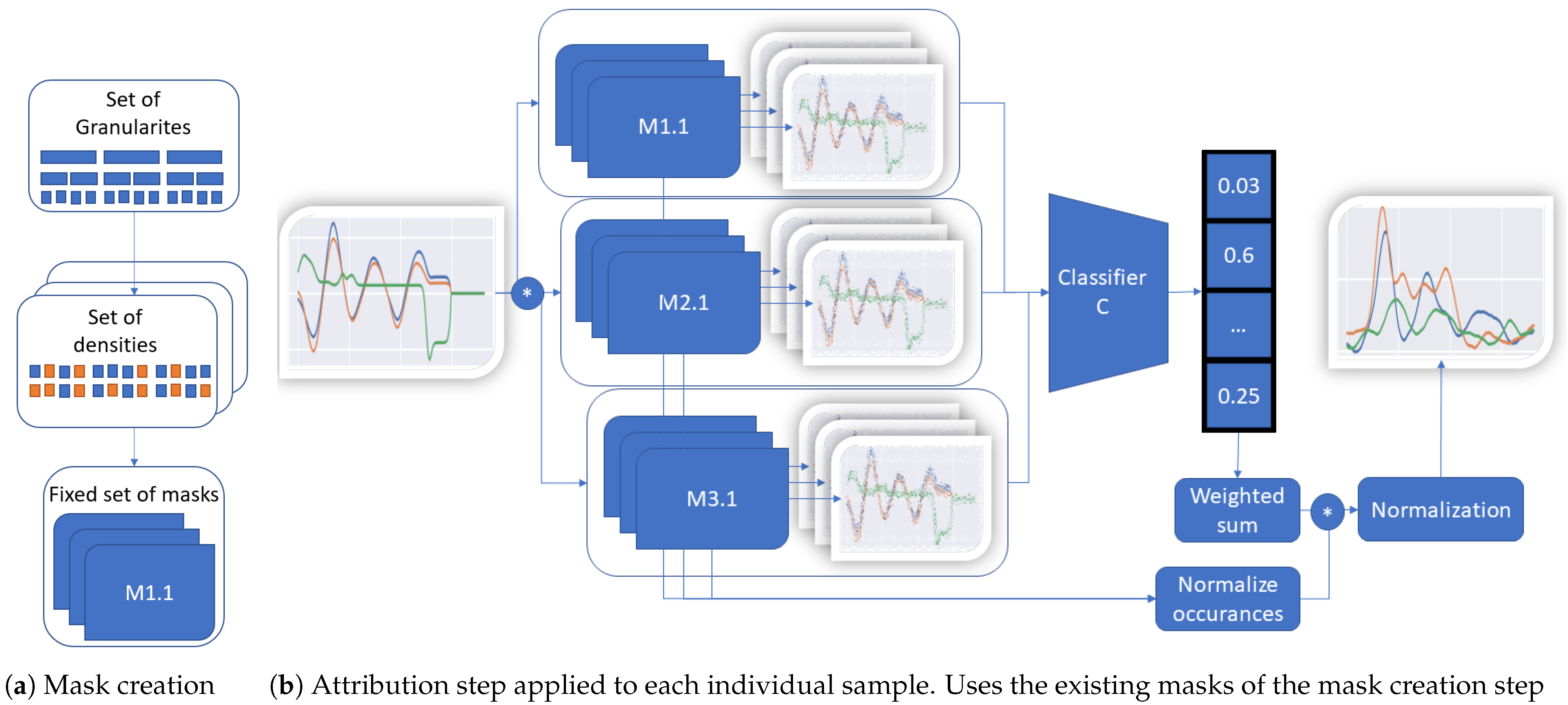
Figure 1.
TimeREISE. Shows the two steps required to use TimeREISE. (a) shows the generation based on a set of different granularities and densities. The granulariy defines the number of slices and the density of the number of perturbed slices within a mask. (b) shows a set of masks (M1.1 to M3.x) applied to the input using an exchangeable perturbation function. The default perturbation is an element.wise multiplication. The masked input is passed to a classifier and the classification score is retrieved. The classification score is multiplied (*) by the masks and normalized by the number of feature occurrences. Finally, the attribution is normalized based on the number of occurrences of each point.
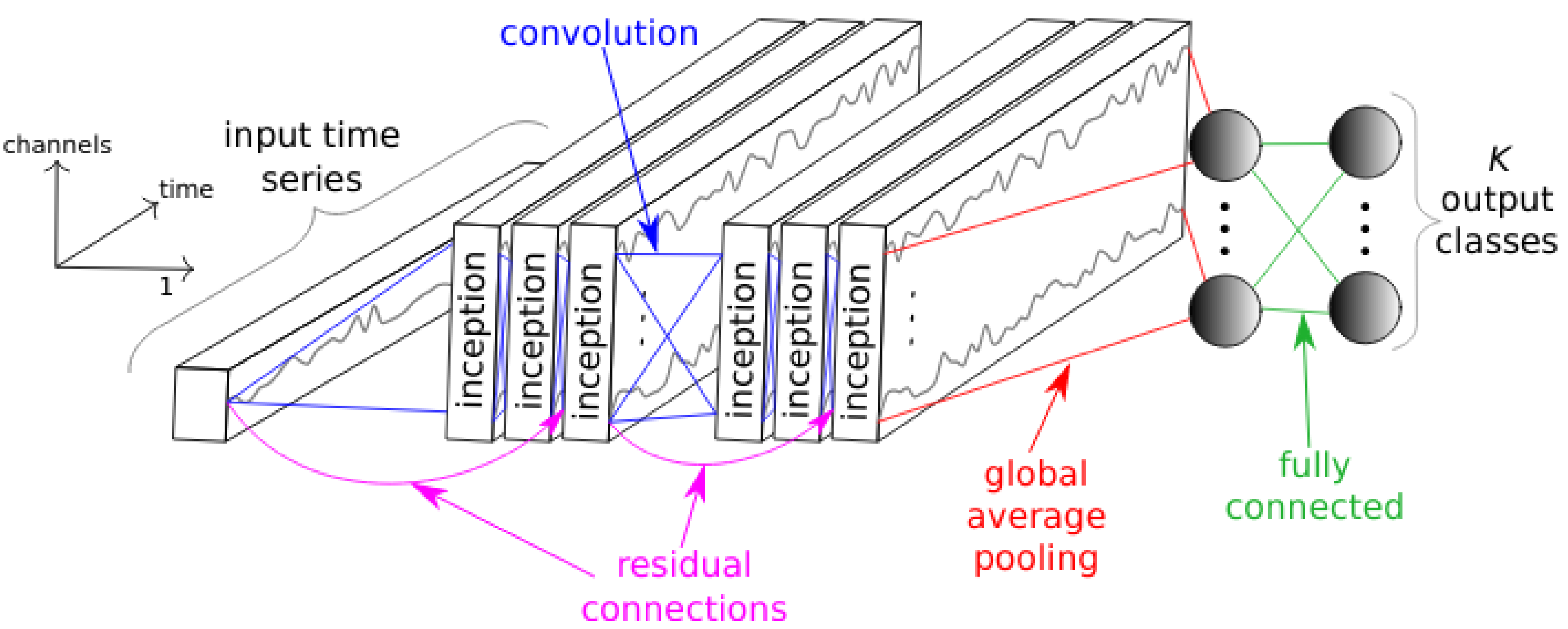
Figure 2.
InceptionTime. Shows the general architecture of InceptionTime proposed by Fawaz et al. [
24]. The architecture shows that there are several inceptionblocks consisting of convoluition layers. Furthermore, the network has residual connections to skip some inceptionblocks. After the last inceptionblock there is a global average pooling followed by a fully connected layer to produce the output classification. Figure taken from [
24].
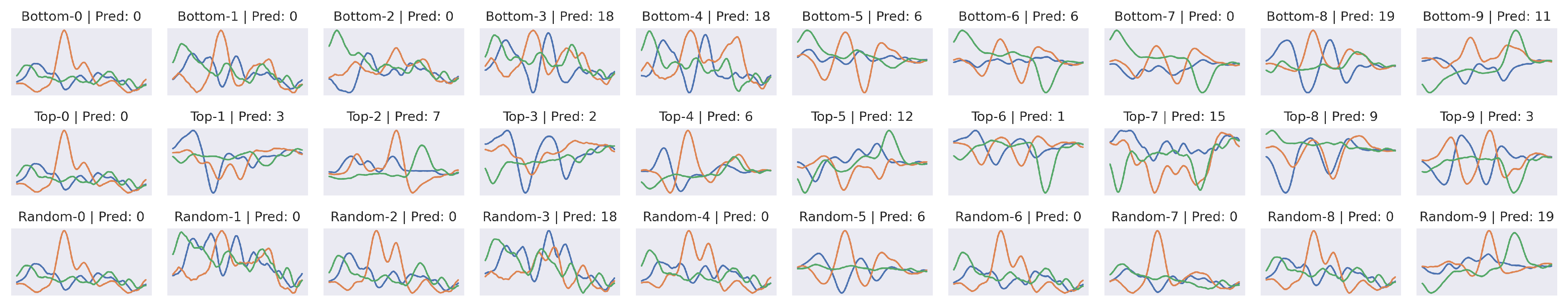
Figure 3.
Sanity Attribution. Shows the attribution map of a CharacterTrajectories sample. Top-X: top-down randomization of X layers, Bottom-X: bottom-up randomization of X layers. Random-X: randomized layer/block X. Top-0 refers to the original attribution map. The results provide evidence that the TimeREISE method strongly depends on the model parameters.
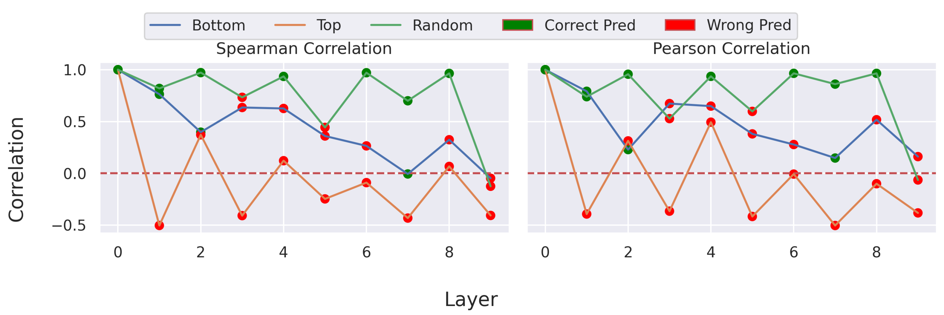
Figure 4.
Sanity Correlation. Shows the correlation between the maps with randomized layers and the original attribution map. Refers to the attribution maps shown in
Figure 3. The figure shows that changes to the network result in a lower correlation of the attribution map compared to the original attribution map.
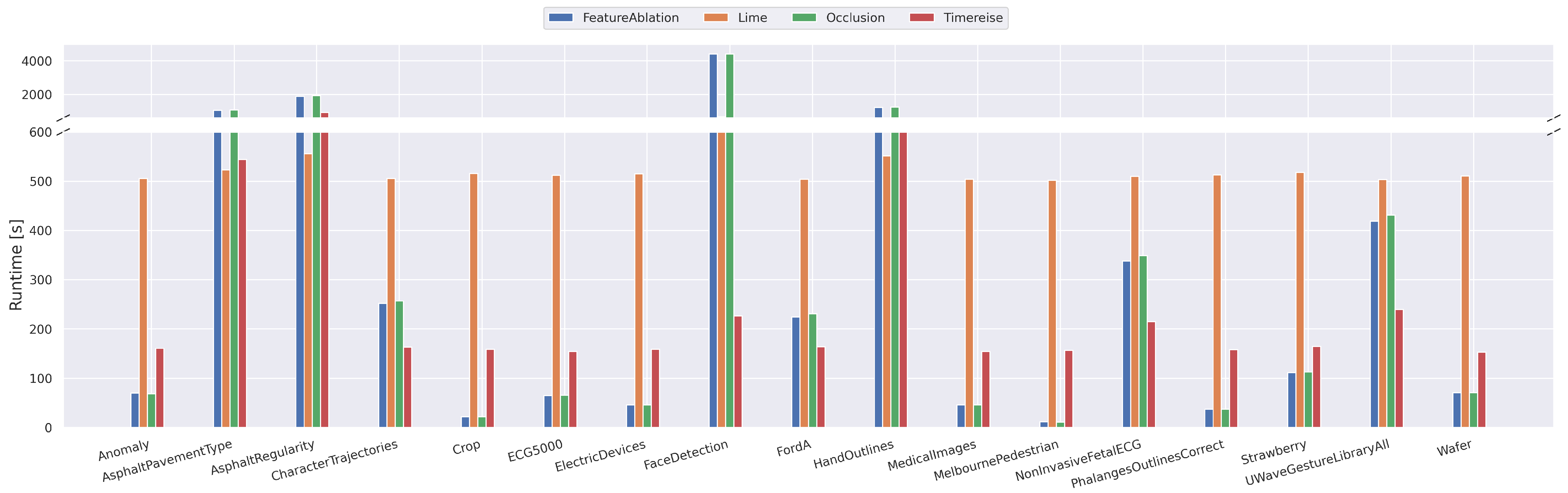
Figure 5.
Runtime Real Data. Shows the runtime on the real datasets used in all experiments below. The runtime is given in seconds for 100 attribution maps. TimeREISE shows a stable runtime across all datasets. For long-sequence datasets the runtime of the other approaches increases.
Figure 5.
Runtime Real Data. Shows the runtime on the real datasets used in all experiments below. The runtime is given in seconds for 100 attribution maps. TimeREISE shows a stable runtime across all datasets. For long-sequence datasets the runtime of the other approaches increases.
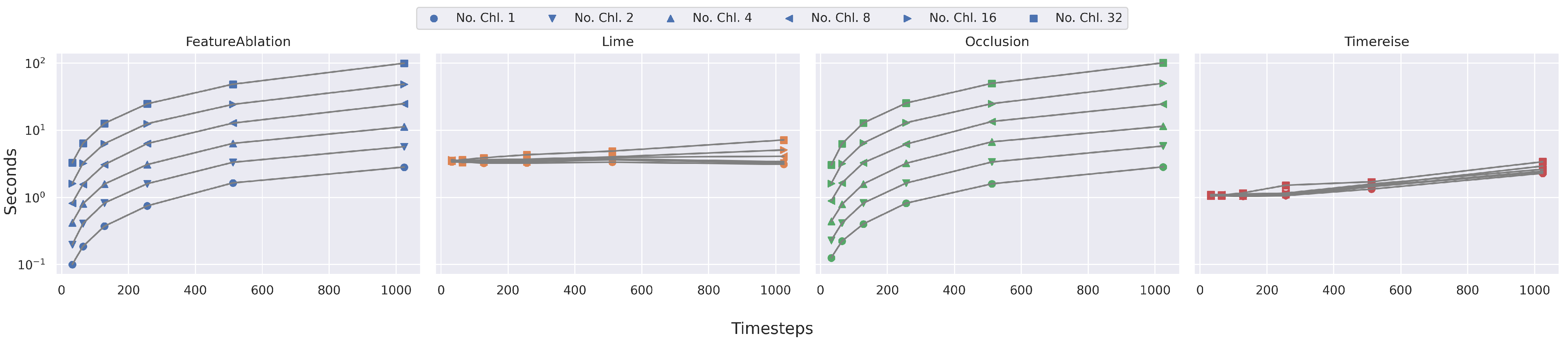
Figure 6.
Runtime Parameter dependency. Shows the runtime on synthetic data with different number of timesteps and channels. IntegratedGradients and GuideBackprop are excluded. The runtime of FeatureAblation and Occlusion increase dramatically with the longer sequences. TimeREISE and Lime show a stable runtime.
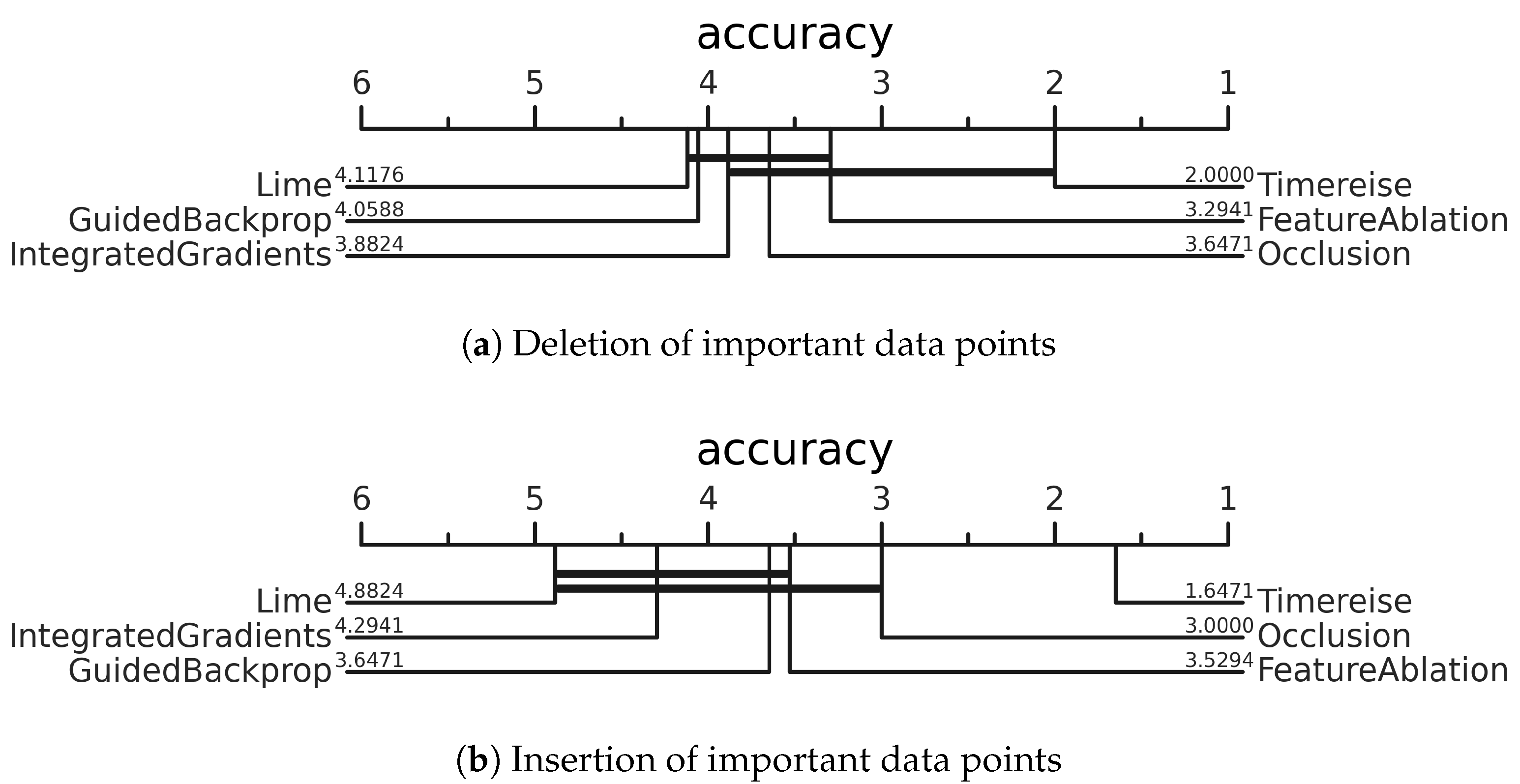
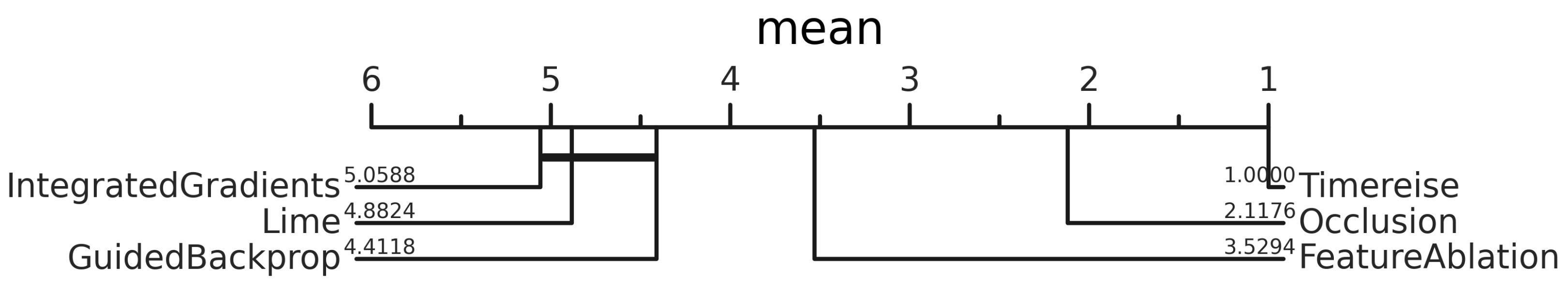
Figure 7.
Deletion & Insertion. Critical difference diagram showing the average rank of each attribution method across all datasets. The ranking is based on the AUC using accuracy. Perturbation-based approaches achieve better results on the deletion and insertion test. TimeREISE shows a superior performance for both tests.
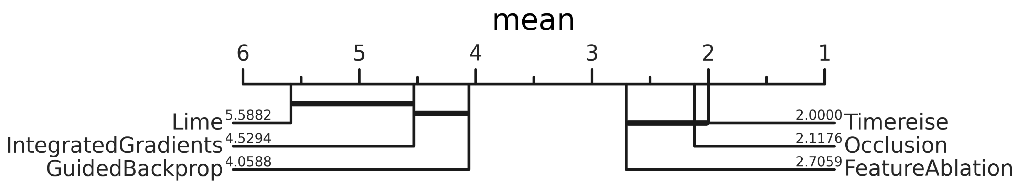
Figure 8.
Sensitivity. A critical difference diagram showing the average rank of each attribution method across all datasets. The ranking is based on the average Sensitivity. Perturbation-based approaches show superior performance. The horizontal bars show the groups that can be concluded based on the rank of the methods. They clearly highlight the high and low performing sets.
Figure 9.
Continuity. Critical difference diagram showing the average rank of each attribution method across all datasets. The ranking is based on the average Continuity. PErturbation-based approaches show superior performance.The horizontal bars show the groups that can be concluded based on the rank of the methods. They clearly highlight the low performing set.
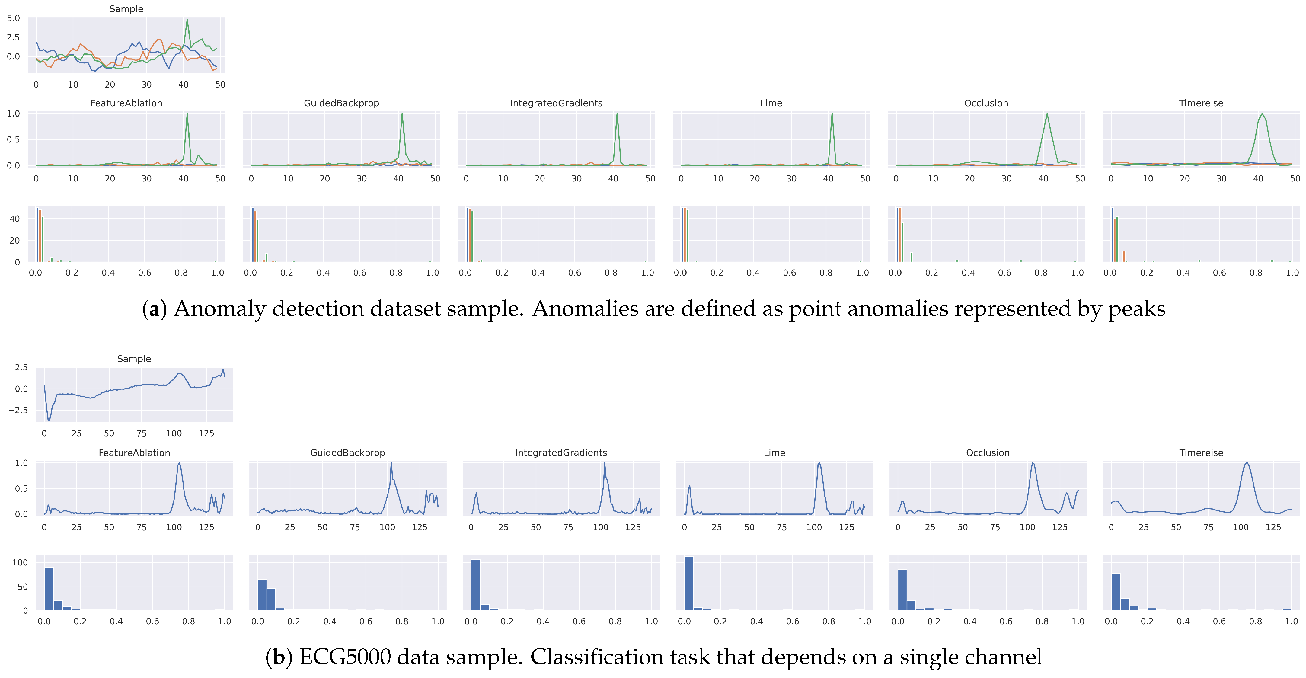
Figure 10.
Attribution Maps. Shows the attribution maps for a single sample. The first row shows the original sample. The second row shows the actual attribution and the third row shows the histogram of the attribution scores within the given map. Generally, a large amount of low values in the histogram relates to a good separation between relevant and irrelevant features. (a) shows an anomalous sample in which the green peak corresponds to the anomalous signal part. Overall the attributions look similar except that TimeREISE is smoother compared to the other methods.
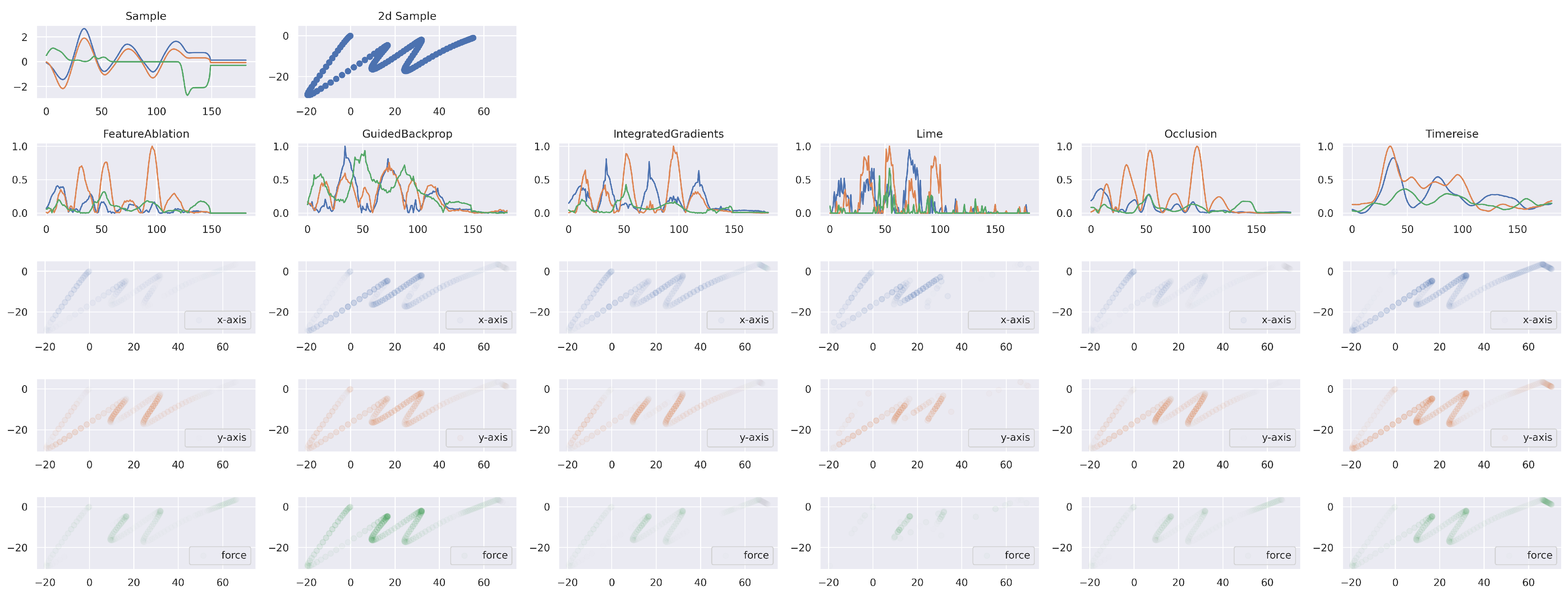
Figure 11.
Explainable Attribution. The first row shows the time series of the character example ‘m’. The right plot corresponds to the back transformation to the original 2d space. The second row shows the attribution results for each method. The subsequent rows show the importance applied to the character for the horizontal and vertical direction as well as for the force. TimeREISE provides a smooth attribution map and assigns importance to the force channel. Besides TimeREISE, only GuidedBackprop highlights the importance of the force channel.
Table 1.
Datasets related to critical infrastructures. Different characteristics such as the datasetsize, length, feature number and classes are covered by this selection.
Table 1.
Datasets related to critical infrastructures. Different characteristics such as the datasetsize, length, feature number and classes are covered by this selection.
| Domain & Dataset | Train | Test | Steps | Channels | Classes |
|---|
| Critical Manufacturing | | | | | |
| Anomaly (synthetic data) | 50,000 | 10,000 | 50 | 3 | 2 |
| ElectricDevices | 8926 | 7711 | 96 | 1 | 7 |
| FordA | 3601 | 1320 | 500 | 1 | 2 |
| Food and Agriculture | | | | | |
| Crop | 7200 | 16,800 | 46 | 1 | 24 |
| Strawberry | 613 | 370 | 235 | 1 | 2 |
| Public Health | | | | | |
| ECG5000 | 500 | 4500 | 140 | 1 | 5 |
| FaceDetection | 5890 | 3524 | 62 | 144 | 2 |
| MedicalImages | 381 | 760 | 99 | 1 | 10 |
| NonInvasiveFetalECG | 1800 | 1965 | 750 | 1 | 42 |
| PhalangesOutlinesCorrect | 1800 | 858 | 80 | 1 | 2 |
| Communications | | | | | |
| CharacterTrajectories | 1422 | 1436 | 182 | 3 | 20 |
| HandOutlines | 1000 | 370 | 2709 | 1 | 2 |
| UWaveGestureLibraryAll | 896 | 3582 | 945 | 1 | 8 |
| Wafer | 1000 | 6164 | 152 | 1 | 2 |
| Transportation Systems | | | | | |
| AsphaltPavementType | 1055 | 1056 | 1543 | 1 | 3 |
| AsphaltRegularity | 751 | 751 | 4201 | 1 | 2 |
| MelbournePedestrian | 1194 | 2439 | 24 | 1 | 10 |
Table 2.
Performance of IncpetionTime. Concerning the accuracy, and f1 scores the subsampled dataset achieves similar performance and can be used as a set of representative samples for further experiments. The results show that the subset accuracy is equal to the complete test set accuracy.
Table 2.
Performance of IncpetionTime. Concerning the accuracy, and f1 scores the subsampled dataset achieves similar performance and can be used as a set of representative samples for further experiments. The results show that the subset accuracy is equal to the complete test set accuracy.
| Dataset | Test Data | 100 Samples |
|---|
| | f1-Macro | f1-Micro | Acc | f1-Macro | f1-Micro | Acc |
|---|
| Anomaly | 0.9769 | 0.9871 | 0.9872 | 0.9699 | 0.9797 | 0.9800 |
| AsphaltPavementType | 0.9169 | 0.9244 | 0.9242 | 0.8905 | 0.8991 | 0.9000 |
| AsphaltRegularity | 1.0000 | 1.0000 | 1.0000 | 1.0000 | 1.0000 | 1.0000 |
| CharacterTrajectories | 0.9940 | 0.9944 | 0.9944 | 1.0000 | 1.0000 | 1.0000 |
| Crop | 0.7189 | 0.7189 | 0.7281 | 0.7058 | 0.7228 | 0.7400 |
| ECG5000 | 0.5611 | 0.9352 | 0.9436 | 0.6045 | 0.9412 | 0.9500 |
| ElectricDevices | 0.6286 | 0.6935 | 0.7056 | 0.6709 | 0.7602 | 0.7900 |
| FaceDetection | 0.6634 | 0.6634 | 0.6637 | 0.6779 | 0.6790 | 0.6800 |
| FordA | 0.9492 | 0.9492 | 0.9492 | 0.9294 | 0.9299 | 0.9300 |
| HandOutlines | 0.9464 | 0.9510 | 0.9514 | 0.9399 | 0.9493 | 0.9500 |
| MedicalImages | 0.7227 | 0.7461 | 0.7474 | 0.7086 | 0.7479 | 0.7500 |
| MelbournePedestrian | 0.9422 | 0.9424 | 0.9422 | 0.9635 | 0.9595 | 0.9600 |
| NonInvasiveFetalECG | 0.9400 | 0.9430 | 0.9425 | 0.8424 | 0.9240 | 0.9200 |
| PhalangesOutlinesCorrect | 0.8142 | 0.8254 | 0.8275 | 0.8849 | 0.8898 | 0.8900 |
| Strawberry | 0.9554 | 0.9593 | 0.9595 | 0.9672 | 0.9699 | 0.9700 |
| UWaveGestureLibraryAll | 0.9165 | 0.9167 | 0.9174 | 0.8525 | 0.8696 | 0.8700 |
| Wafer | 0.9954 | 0.9982 | 0.9982 | 1.0000 | 1.0000 | 1.0000 |
| Average | 0.8613 | 0.8911 | 0.8931 | 0.8593 | 0.8954 | 0.8988 |
Table 3.
Deletion & Insertion. Sequential deletion of the most important points from the original input signal. Respectively, sequential insertion of the most important points starts with a sample consisting of mean values. Lower AUC scores are better for deletion. Higher AUC scores are better for insertion. AUC was calculated using classification accuracy. TimeREISE outperforms any other methods concerning the deletion and achieves the best average for both deletion and insertion. Best results are highlighted in bold.
| Dataset | FeatureAblation [16] | GuidedBackprop [14] | IntegratedGrad. [15] | Lime [18] | Occlusion [17] | TimeREISE (Ours) |
|---|
| | del | ins | del | ins | del | ins | del | ins | del | ins | del | ins |
|---|
| Anomaly | 0.7731 | 0.9737 | 0.7791 | 0.9597 | 0.7786 | 0.9624 | 0.7783 | 0.9473 | 0.7714 | 0.9739 | 0.7631 | 0.9867 |
| AsphaltPavementType | 0.4073 | 0.8819 | 0.3930 | 0.8944 | 0.3940 | 0.8935 | 0.4622 | 0.8623 | 0.4171 | 0.8726 | 0.4135 | 0.8641 |
| AsphaltRegularity | 0.5857 | 0.9954 | 0.5785 | 0.9960 | 0.5817 | 0.9964 | 0.6843 | 0.9871 | 0.5901 | 0.9929 | 0.5927 | 0.9833 |
| CharacterTrajectories | 0.0856 | 0.8563 | 0.0807 | 0.8701 | 0.1091 | 0.8580 | 0.0785 | 0.8543 | 0.0878 | 0.8609 | 0.0401 | 0.8809 |
| Crop | 0.0998 | 0.3780 | 0.1402 | 0.3026 | 0.1404 | 0.2652 | 0.1096 | 0.3198 | 0.1583 | 0.3170 | 0.0628 | 0.5065 |
| ECG5000 | 0.2104 | 0.8771 | 0.1876 | 0.8782 | 0.1208 | 0.8792 | 0.1294 | 0.8846 | 0.1176 | 0.8796 | 0.1015 | 0.9060 |
| ElectricDevices | 0.3086 | 0.5393 | 0.3616 | 0.5718 | 0.3178 | 0.5244 | 0.3338 | 0.4971 | 0.3524 | 0.5914 | 0.2726 | 0.6957 |
| FaceDetection | 0.5165 | 0.6760 | 0.2462 | 0.8065 | 0.5116 | 0.6660 | 0.6019 | 0.6308 | 0.5281 | 0.6691 | 0.0080 | 0.9968 |
| FordA | 0.4729 | 0.7816 | 0.4829 | 0.8207 | 0.4793 | 0.6834 | 0.4803 | 0.6731 | 0.4751 | 0.8493 | 0.3859 | 0.9436 |
| HandOutlines | 0.3125 | 0.3630 | 0.3137 | 0.3289 | 0.3127 | 0.3432 | 0.3153 | 0.3201 | 0.3107 | 0.3911 | 0.3485 | 0.3607 |
| MedicalImages | 0.1840 | 0.5884 | 0.1588 | 0.5645 | 0.1953 | 0.4518 | 0.1736 | 0.5622 | 0.1569 | 0.5883 | 0.1229 | 0.7125 |
| MelbournePedestrian | 0.1579 | 0.5967 | 0.2071 | 0.5579 | 0.2733 | 0.4579 | 0.1767 | 0.6013 | 0.2363 | 0.4763 | 0.0979 | 0.6538 |
| NonInvasiveFetalECG | 0.0424 | 0.1488 | 0.0454 | 0.0654 | 0.0405 | 0.0868 | 0.0462 | 0.0816 | 0.0422 | 0.2503 | 0.0894 | 0.4333 |
| PhalangesOutlinesCorrect | 0.4033 | 0.5072 | 0.4058 | 0.4347 | 0.4056 | 0.4437 | 0.4038 | 0.4288 | 0.4034 | 0.5616 | 0.2919 | 0.6171 |
| Strawberry | 0.5827 | 0.7179 | 0.6141 | 0.7100 | 0.6428 | 0.7179 | 0.6397 | 0.7087 | 0.5958 | 0.7761 | 0.3882 | 0.7909 |
| UWaveGestureLibraryAll | 0.1840 | 0.4243 | 0.1353 | 0.5260 | 0.1285 | 0.1452 | 0.1226 | 0.1782 | 0.1743 | 0.4669 | 0.0973 | 0.5379 |
| Wafer | 0.2740 | 0.7684 | 0.3441 | 0.8574 | 0.2603 | 0.8061 | 0.2324 | 0.8613 | 0.2642 | 0.7932 | 0.2002 | 0.8976 |
| Average | 0.3295 | 0.6514 | 0.3220 | 0.6556 | 0.3348 | 0.5989 | 0.3393 | 0.6117 | 0.3342 | 0.6653 | 0.2516 | 0.7510 |
Table 4.
Infidelity. Lower values correspond to better performance. The Method names are shortened by taking only the initial character (FeatureAblation, Guided-Backpropagation, IntegratedGradients, LIME, Occlusion, TimeREISE). There are only insignificant differences between the methods. Lime shows the best performance. TimeREISE takes the second place. Best results are highlighted in bold.
| Dataset | F [16] | G [14] | I [15] | L [18] | O [17] | T (Ours) |
|---|
| Anomaly | 0.0233 | 0.0193 | 0.0158 | 0.0184 | 0.0222 | 0.0230 |
| AsphaltPavementType | 0.2126 | 0.2126 | 0.2126 | 0.2127 | 0.2126 | 0.2124 |
| AsphaltRegularity | 0.0045 | 0.0046 | 0.0046 | 0.0046 | 0.0045 | 0.0045 |
| CharacterTrajectories | 0.1399 | 0.1397 | 0.1399 | 0.1399 | 0.1399 | 0.1396 |
| Crop | 0.2967 | 0.3081 | 0.3055 | 0.2966 | 0.3143 | 0.3032 |
| ECG5000 | 0.0273 | 0.0272 | 0.0257 | 0.0210 | 0.0236 | 0.0242 |
| ElectricDevices | 18.0869 | 18.1047 | 18.1130 | 18.1042 | 18.0854 | 18.1070 |
| FaceDetection | 0.0002 | 0.0002 | 0.0002 | 0.0002 | 0.0002 | 0.0002 |
| FordA | 0.0118 | 0.0118 | 0.0116 | 0.0116 | 0.0118 | 0.0118 |
| HandOutlines | 1.6914 | 1.7015 | 1.6932 | 1.6928 | 1.6938 | 1.6920 |
| MedicalImages | 0.2492 | 0.2492 | 0.2472 | 0.2486 | 0.2490 | 0.2482 |
| MelbournePedestrian | 1.2324 | 1.2833 | 1.3745 | 1.1959 | 1.3319 | 1.2301 |
| NonInvasiveFetalECG | 51.7361 | 51.7288 | 51.7252 | 51.7228 | 51.7413 | 51.7072 |
| PhalangesOutlinesCorrect | 0.4394 | 0.4285 | 0.4360 | 0.4413 | 0.4403 | 0.4405 |
| Strawberry | 0.4865 | 0.4783 | 0.4863 | 0.4849 | 0.4811 | 0.4851 |
| UWaveGestureLibraryAll | 4.9995 | 4.9983 | 4.9922 | 4.9996 | 4.9992 | 4.9968 |
| Wafer | 0.0355 | 0.0356 | 0.0355 | 0.0356 | 0.0355 | 0.0352 |
| Average | 4.6867 | 4.6901 | 4.6952 | 4.6842 | 4.6933 | 4.6859 |
Table 5.
Sensitivity. Lower values correspond to better performance. The method names are shortened by taking only the initial character (FeatureAblation, Guided-Backpropagation, IntegratedGradients, LIME, Occlusion, TimeREISE). Perturbation-based approaches show superior performance. TimeREISE shows the best performance across most of the datasets. Best results are highlighted in bold.
| Dataset | F [16] | G [14] | I [15] | L [18] | O [17] | T (Ours) |
|---|
| Anomaly | 0.0574 | 0.0747 | 0.1470 | 0.2591 | 0.0664 | 0.0522 |
| AsphaltPavementType | 0.0292 | 0.2864 | 0.0358 | 0.4259 | 0.0274 | 0.0705 |
| AsphaltRegularity | 0.0288 | 0.2797 | 0.0567 | 0.3664 | 0.0274 | 0.0028 |
| CharacterTrajectories | 0.0199 | 0.0547 | 0.0705 | 0.1353 | 0.0174 | 0.0076 |
| Crop | 0.0808 | 0.1060 | 0.1702 | 0.1786 | 0.1307 | 0.0411 |
| ECG5000 | 0.0301 | 0.0772 | 0.1218 | 0.1811 | 0.0248 | 0.0111 |
| ElectricDevices | 0.2069 | 0.2608 | 0.6129 | 0.2622 | 0.1949 | 0.1696 |
| FaceDetection | 0.0180 | 0.0204 | 0.0136 | 0.4722 | 0.0144 | 0.0048 |
| FordA | 0.0231 | 0.0384 | 0.0708 | 0.1690 | 0.0155 | 0.0147 |
| HandOutlines | 0.0952 | 0.1545 | 0.1203 | 0.1249 | 0.0743 | 0.1175 |
| MedicalImages | 0.0428 | 0.0680 | 0.1483 | 0.1754 | 0.0395 | 0.0406 |
| MelbournePedestrian | 0.1667 | 0.1363 | 0.1684 | 0.2514 | 0.2176 | 0.0472 |
| NonInvasiveFetalECG | 0.1142 | 0.1043 | 0.1543 | 0.1564 | 0.0869 | 0.1570 |
| PhalangesOutlinesCorrect | 0.0415 | 0.1442 | 0.1562 | 0.1212 | 0.0390 | 0.0574 |
| Strawberry | 0.0486 | 0.0966 | 0.0506 | 0.1267 | 0.0515 | 0.0698 |
| UWaveGestureLibraryAll | 0.0569 | 0.0535 | 0.2341 | 0.1778 | 0.0373 | 0.0381 |
| Wafer | 0.0252 | 0.0368 | 0.1299 | 0.1250 | 0.0141 | 0.0051 |
| Average | 0.0638 | 0.1172 | 0.1448 | 0.2182 | 0.0635 | 0.0533 |
Table 6.
Continuity. Lower values correspond to better performance. The method names are shortened by taking only the initial character (FeatureAblation, Guided-Backpropagation, IntegratedGradients, LIME, Occlusion, TimeREISE). TimeREISE shows a superior performance across all datasets. Best results are highlighted in bold.
| Dataset | F [16] | G [14] | I [15] | L [18] | O [17] | T (Ours) |
|---|
| Anomaly | 0.1163 | 0.1444 | 0.1309 | 0.1390 | 0.0908 | 0.0473 |
| AsphaltPavementType | 0.0792 | 0.0977 | 0.0770 | 0.0765 | 0.0450 | 0.0015 |
| AsphaltRegularity | 0.0582 | 0.0703 | 0.0485 | 0.0525 | 0.0334 | 0.0008 |
| CharacterTrajectories | 0.0264 | 0.0324 | 0.0368 | 0.0619 | 0.0243 | 0.0134 |
| Crop | 0.1282 | 0.1655 | 0.1952 | 0.1741 | 0.0985 | 0.0618 |
| ECG5000 | 0.0682 | 0.1000 | 0.1004 | 0.0844 | 0.0505 | 0.0296 |
| ElectricDevices | 0.2016 | 0.1840 | 0.1984 | 0.1950 | 0.0884 | 0.0350 |
| FaceDetection | 0.0690 | 0.0745 | 0.0613 | 0.0331 | 0.0373 | 0.0161 |
| FordA | 0.0770 | 0.0819 | 0.0959 | 0.1530 | 0.0576 | 0.0083 |
| HandOutlines | 0.0123 | 0.0183 | 0.0258 | 0.1501 | 0.0106 | 0.0015 |
| MedicalImages | 0.0923 | 0.1043 | 0.1259 | 0.1076 | 0.0602 | 0.0371 |
| MelbournePedestrian | 0.1804 | 0.1844 | 0.2217 | 0.1881 | 0.1264 | 0.1052 |
| NonInvasiveFetalECG | 0.0224 | 0.0650 | 0.0753 | 0.1603 | 0.0197 | 0.0043 |
| PhalangesOutlinesCorrect | 0.1066 | 0.1187 | 0.1525 | 0.1416 | 0.0715 | 0.0496 |
| Strawberry | 0.0720 | 0.0679 | 0.0785 | 0.1447 | 0.0676 | 0.0159 |
| UWaveGestureLibraryAll | 0.0216 | 0.0557 | 0.0816 | 0.1629 | 0.0226 | 0.0038 |
| Wafer | 0.0924 | 0.0957 | 0.1418 | 0.1222 | 0.0557 | 0.0232 |
| Average | 0.0838 | 0.0977 | 0.1087 | 0.1263 | 0.0565 | 0.0267 |


