
Detection and Classification of Artifact Distortions in Optical Motion Capture Sequences


Abstract
:1. Introduction
2. Background
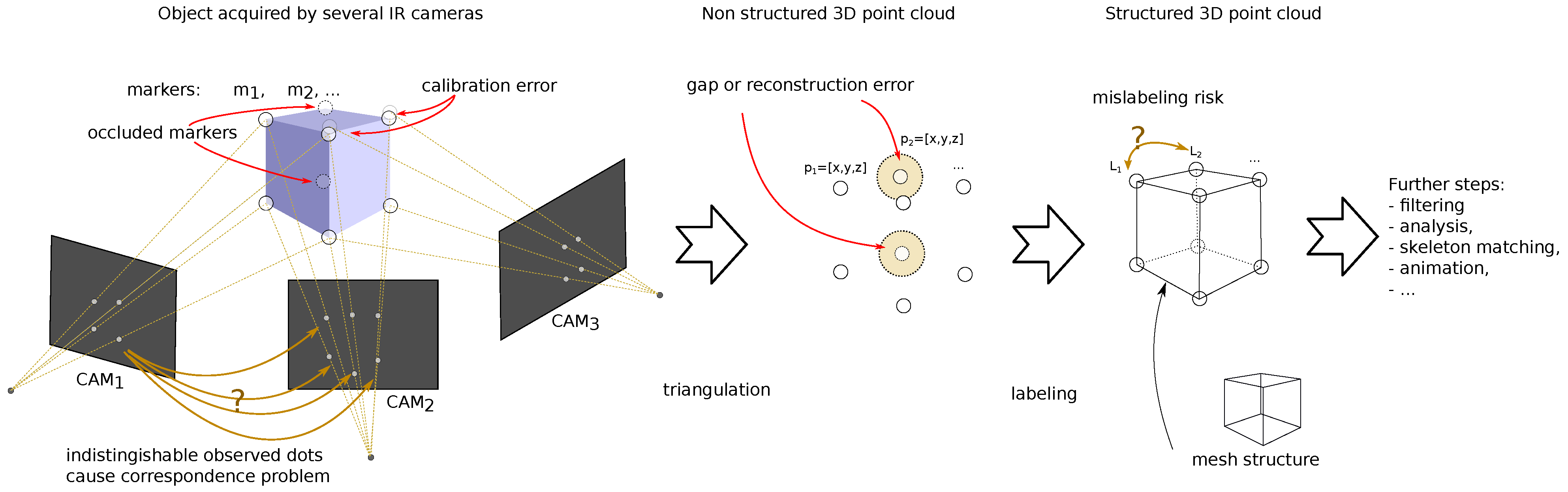
2.1. Sources and Types of Distortions
- 1.
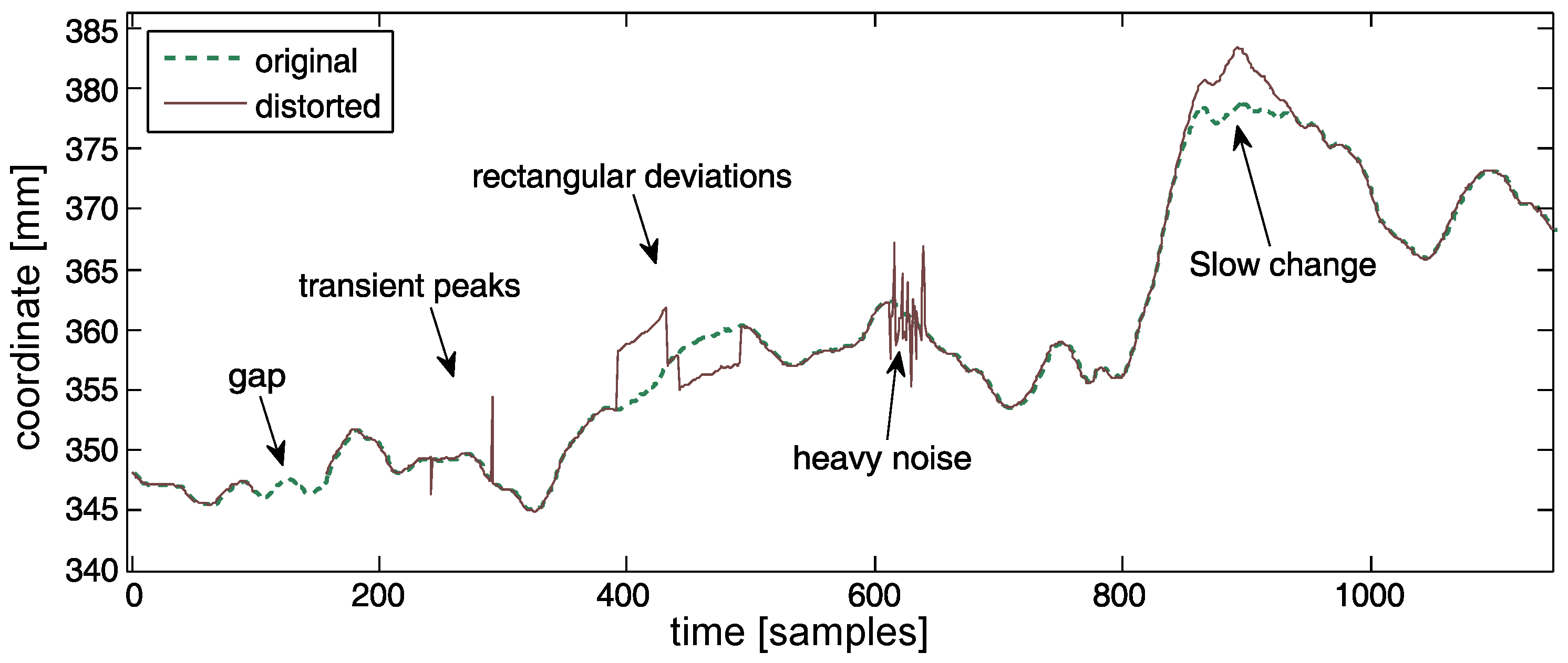
- Simple gap—appears when reconstruction algorithms give up, it is the least type of concern (a trivial case);
- 2.
- Single peak—caused by transient erroneous marker matching techniques. It is simple to detect;
- 3.
- Heavy noise of a much larger amplitude than ordinary noise introduced by frequent erroneous marker matching techniques;
- 4.
- Rectangular distortion—forward (followed by backward) steps caused by mismatching the 3D positions of the markers (part of the 3D trajectory is assigned to another marker) or due to the erroneous marker reconstruction based on a rigid body model;
- 5.
- Slow value change—two potential sources—accumulated reconstruction errors in successive frames (e.g., when there is deformation of a body, which is the failure of a commonly assumed rigid body model) or the result of low-pass filtering of peaks.
2.2. Previous Work
3. The Proposal
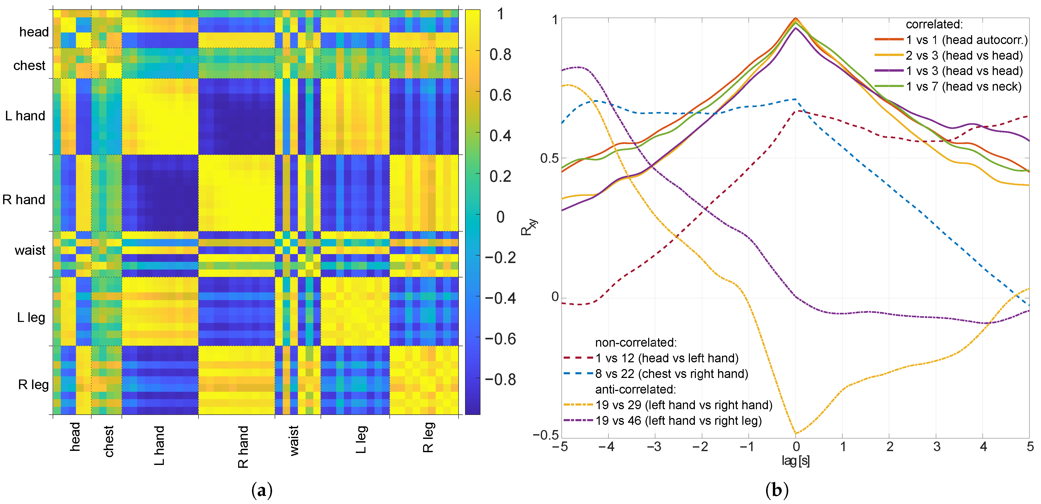
3.1. Premises—Correlation of Trajectory Coordinates
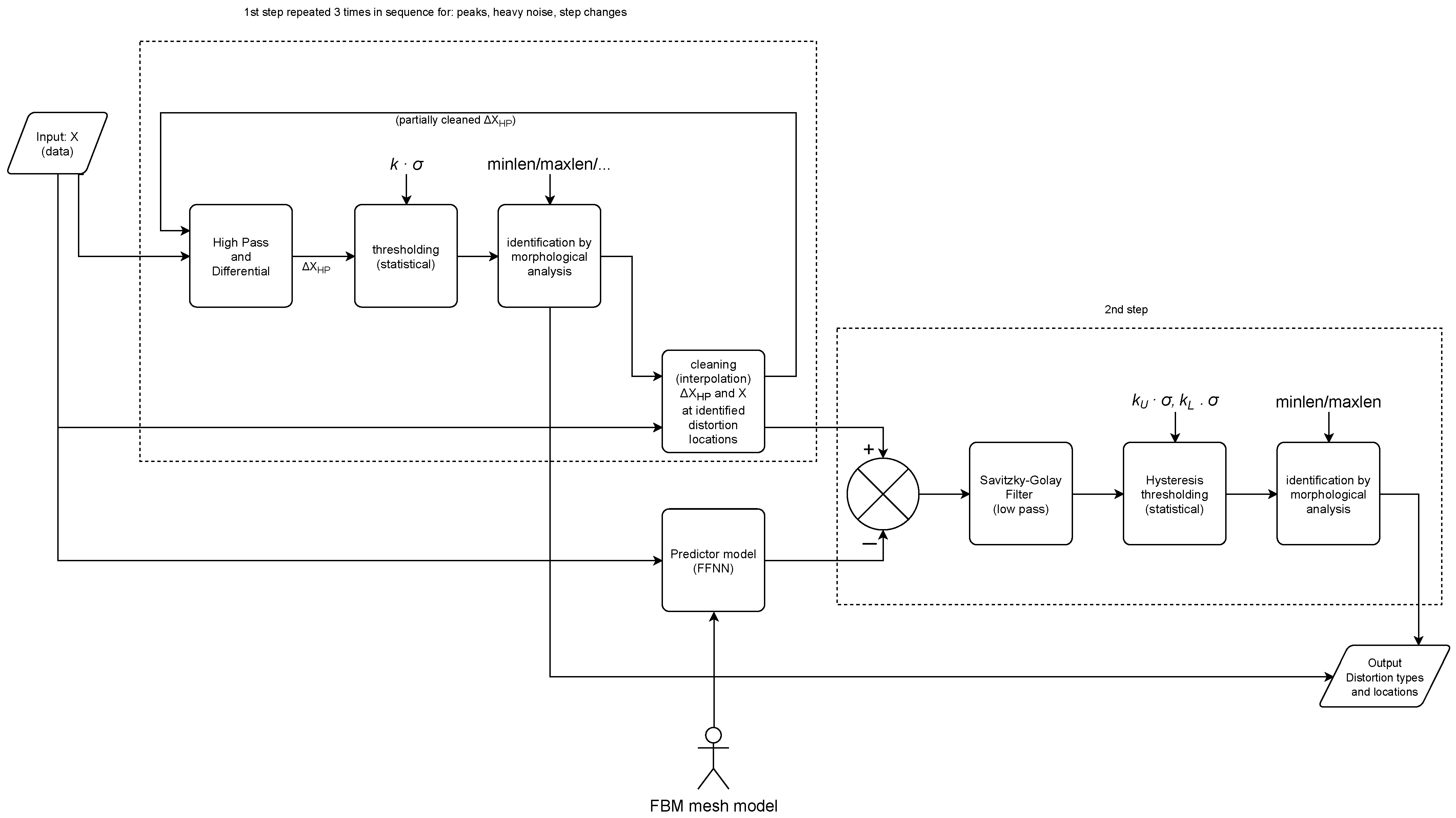
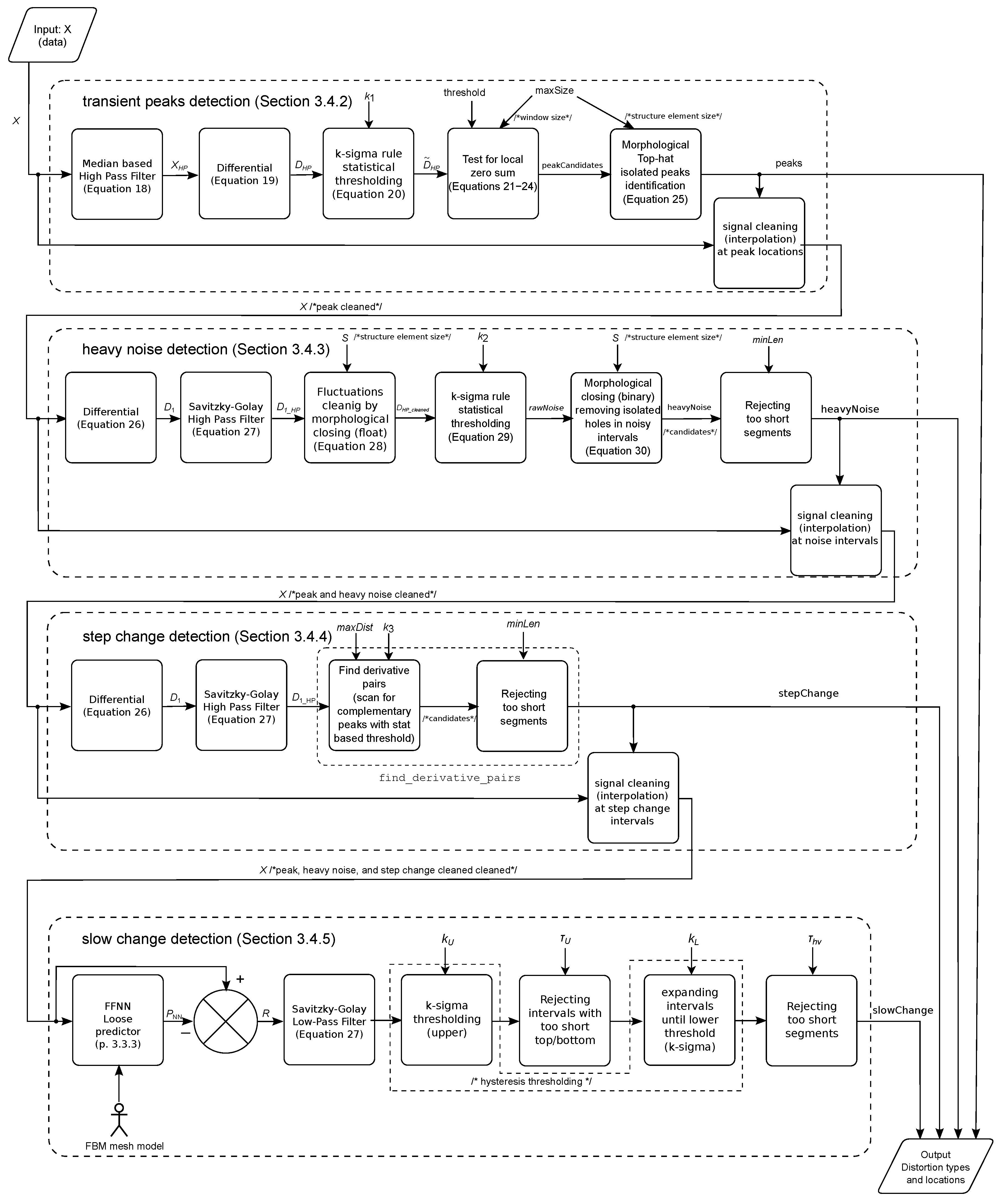
3.2. The Method Overview
3.3. Regressive Models
3.3.1. Savitzky–Golay Filter
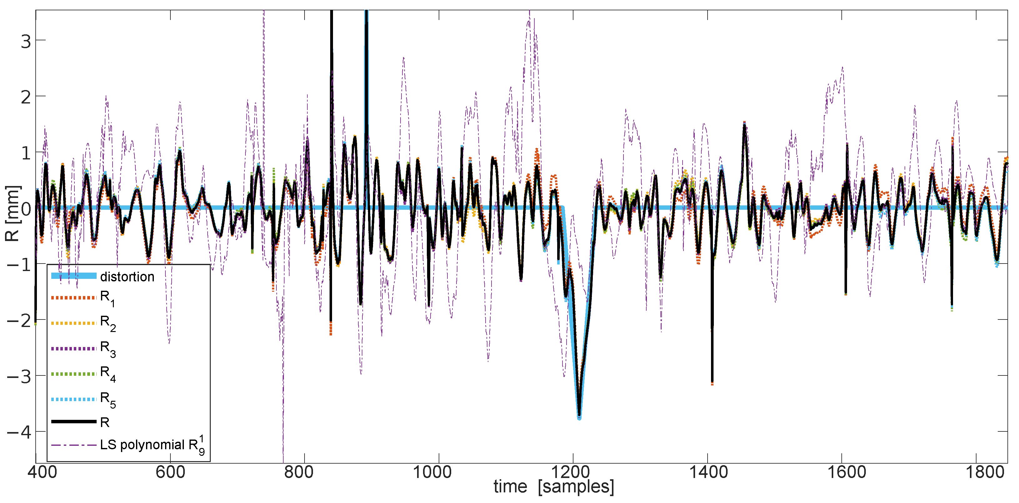
3.3.2. Neighbor-Based Linear Least Squares Loose Model
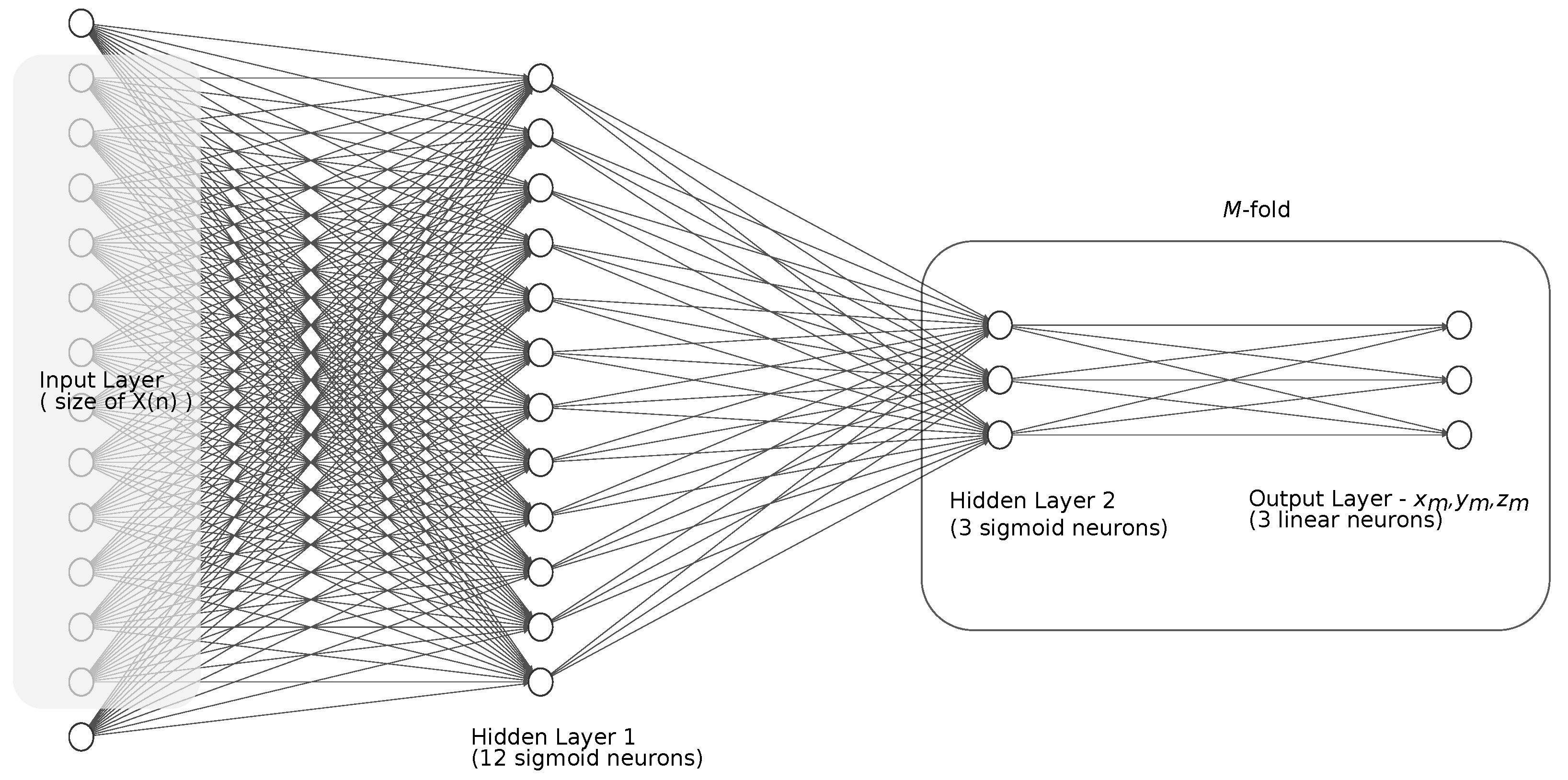
3.3.3. Regression with Neural Network
3.4. Recognition and Classification of Distortions
3.4.1. Locating Sudden Changes
3.4.2. Identifying Single Peaks
- —for the moving average, we assumed it to be 19 samples long;
- —it is calculated statistically from the data using of —w employed as a default value; however, any can be provided as the parameter;
- —(anti-sensitivity) for the ;
- —(default 5), which declares the maximal size of the expected peaks; it affects the size of moving sum windows , which is samples long, it also defines the size of the linear structuring element for morphological operations S.
3.4.3. Heavy Noise
- —this is calculated statistically from the data using of —w employed as a default value; however, any k can be provided as parameter;
- Minimal length of the segment (), which is used to define the linear structuring element S as ; we assumed samples;
- Default parameters of Savitzky–Golay are L = 5, M = 13.
3.4.4. Step Change
- —this is calculated statistically from using of—we employed as a default value; however, any can be provided as parameter,
- Minimal length of the segment (); we assumed samples;
- Maximal searching distance ; we assumed 200 samples as the default value.
- Default parameters of Savitzky–Golay are the same as for heavy noise L = 5, M = 13.
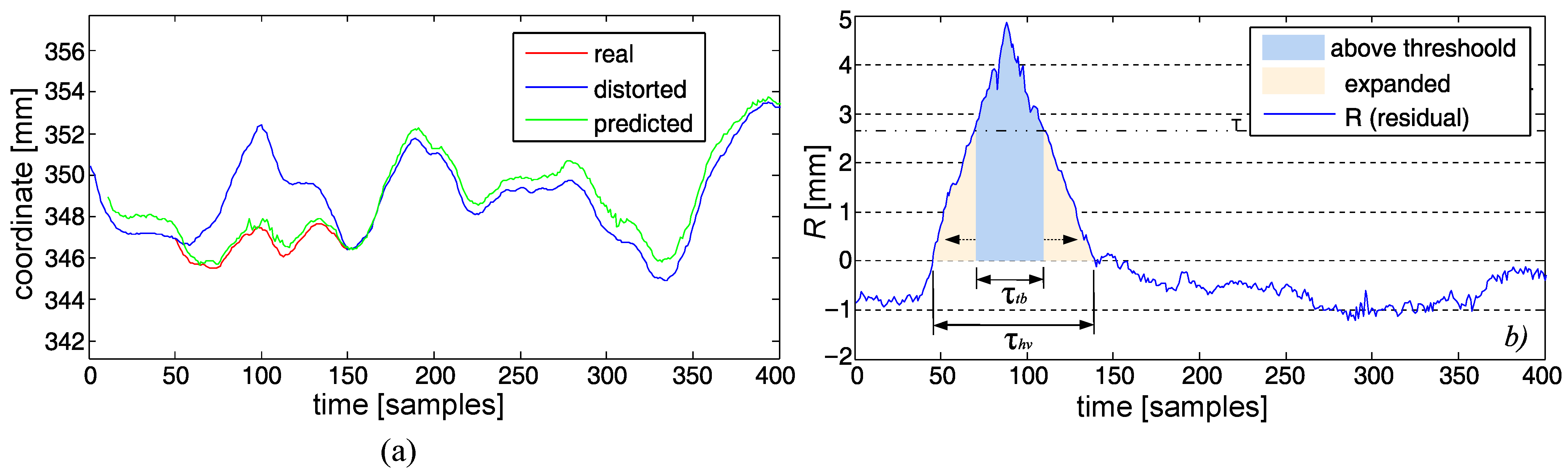
3.4.5. Identifying Slow Changes
- 1.
- Smoothed the R with the Savitzky–Golay low-pass filter (L = 7, M = 11—parameters heuristically tuned).
- 2.
- The upper threshold was set up with a rule of a thumb—in our case, three times was selected () as the default would identify the significant tops and bottoms of the hills and valleys.
- 3.
- If the top or bottom lengths were shorter than some minimal , we skipped it (0.2 s—20 frames in our case), assuming it to be short-term fluctuation.
- 4.
- After the identification of a top/bottom value, we looked for the rest of a distortion (below threshold)—the marked range expanded both sides iteratively (in the past and future) until the residual value went below/above the lower threshold , obtained with with as the default value.
- 5.
- If the overall located distortion (hill/valley) was shorter than some value (50 frames—0.5 s), it was omitted, as one can consider it a short-term fluctuation of the predictor.
4. Verification of the Method
4.1. Materials and Methods
4.1.1. The Data
4.1.2. Experimental Protocols
4.1.3. Artifact Contamination Procedure
- The sign was a +1/−1 value drawn with equal probabilities;
- The amplitude was a Gaussian random variable with assumed amplitude and standard deviation (in the tested cases: mm and ); these values were used to scale the peak of the rectangle or triangle distortion and as the standard deviations in the heavy noise area;
- Distortion durations and intervals were part of the Poisson process; an average length of distortion was set up to 50 samples, and the interval length was adjusted according to the duration of the sequence and the target amount of the given distortion.
4.2. Results and Discussion
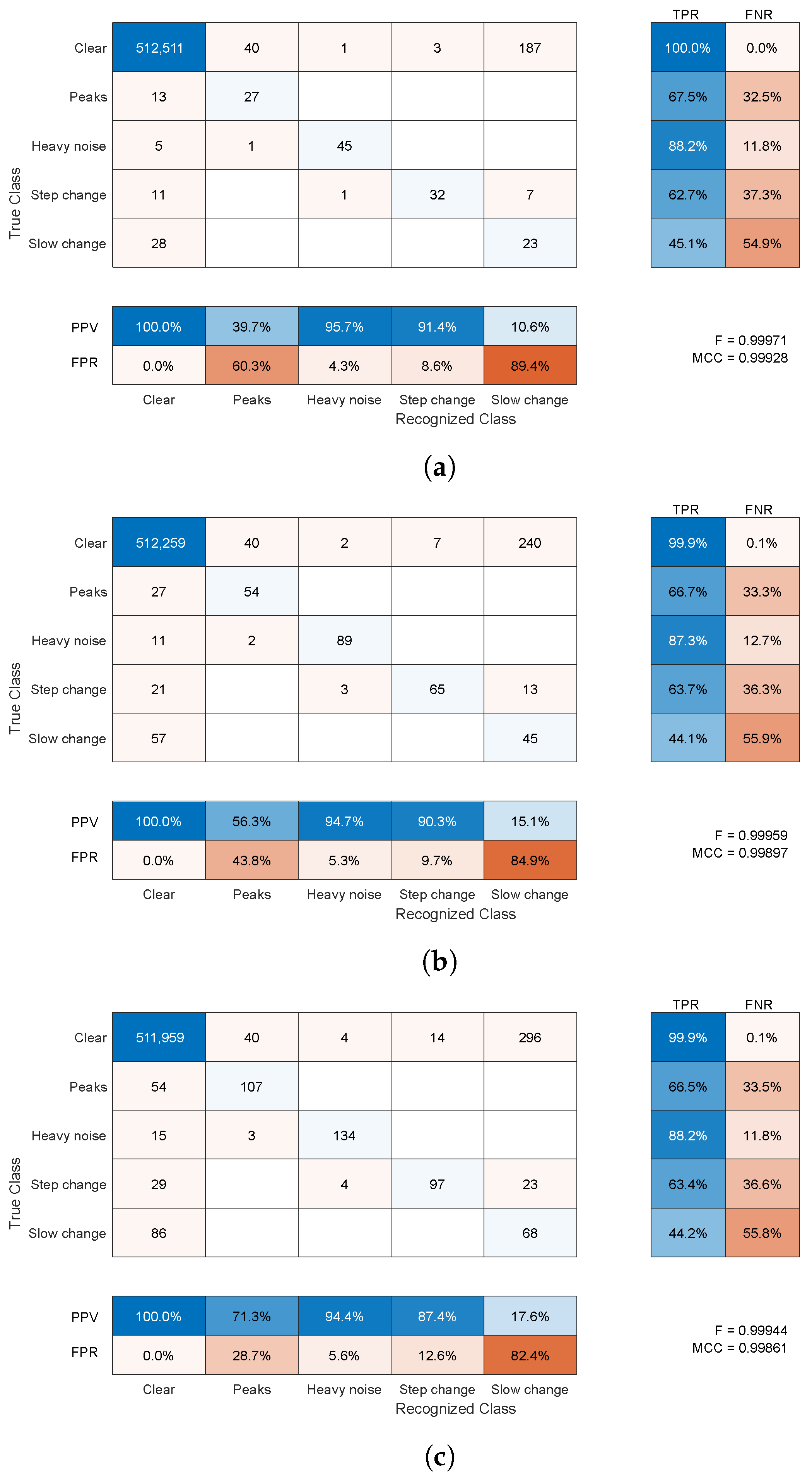
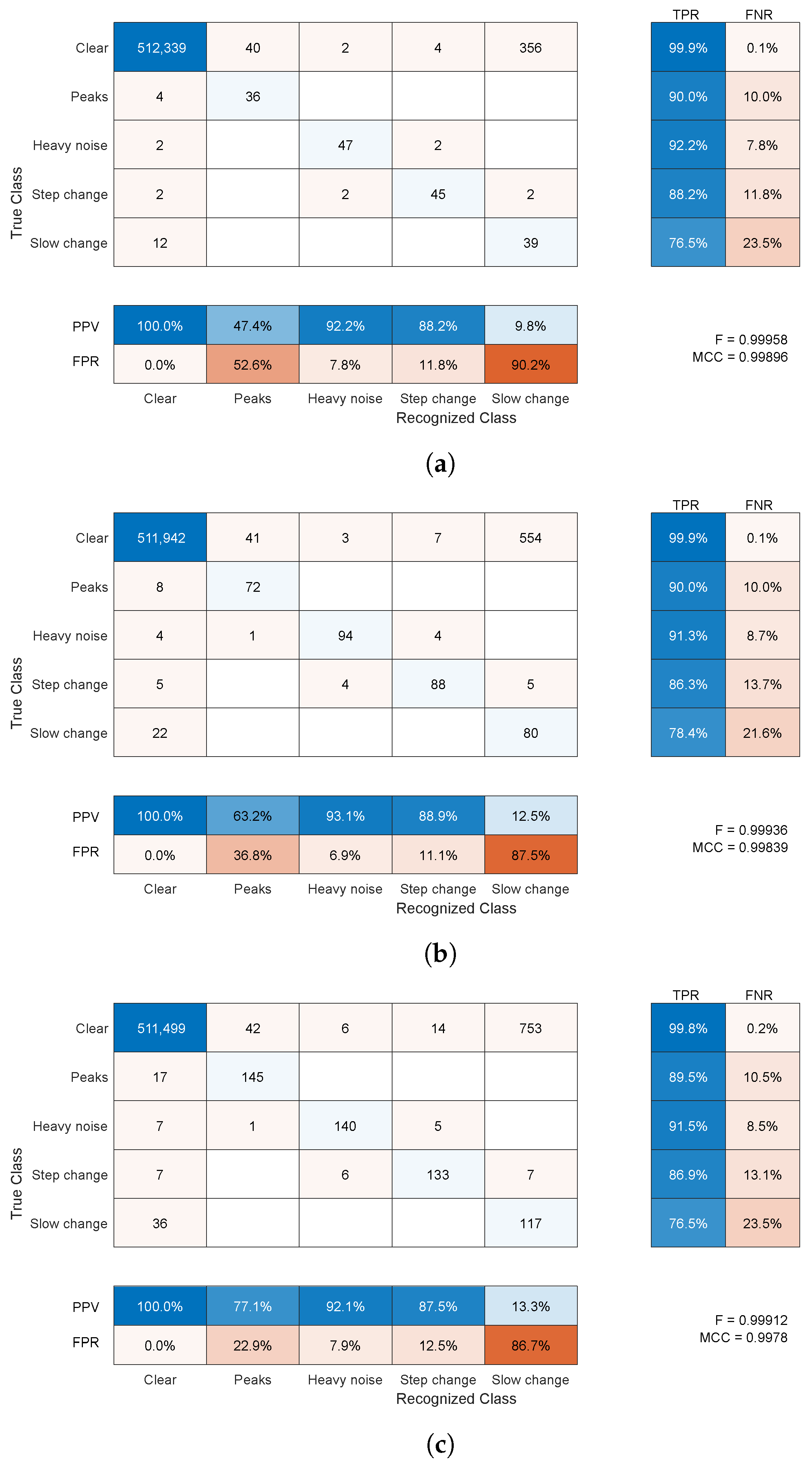
4.2.1. Synthetic Distortion Classification
- The clear signal was identified properly for more than 99% of samples; a negligibly small amount of distorted samples was erroneously identified as clean signals (compared to the overall cardinality of the class).
- For the peak change, sensitivity was approximately 66% and 90%, and the main misclassification was in a clear signal; this class was not a cause of confusion for the other classes compared to a clean signal (usually below ).
- Heavy noise sensitivity was above 88%; the main confusions were step change and a clear signal; this class was rarely erroneously recognized in place of the others ( = 4–8%); the main confused class was a clear signal.
- For the step change, sensitivity was approximately 70% and the main confusion was slow change; this class was erroneously recognized in place of others at a moderate rate ( = 12–27%)—here, a clean signal and heavy noise were wrongly identified.
- For the slow change, was a bit more than 50% and the main confusion was a clear signal; this class was often difficult and erroneously recognized in place of others ( = 80–90%)—usually, it was a clear signal, but a step change and heavy noise were also wrongly identified.
4.2.2. Comparing to Human Operators
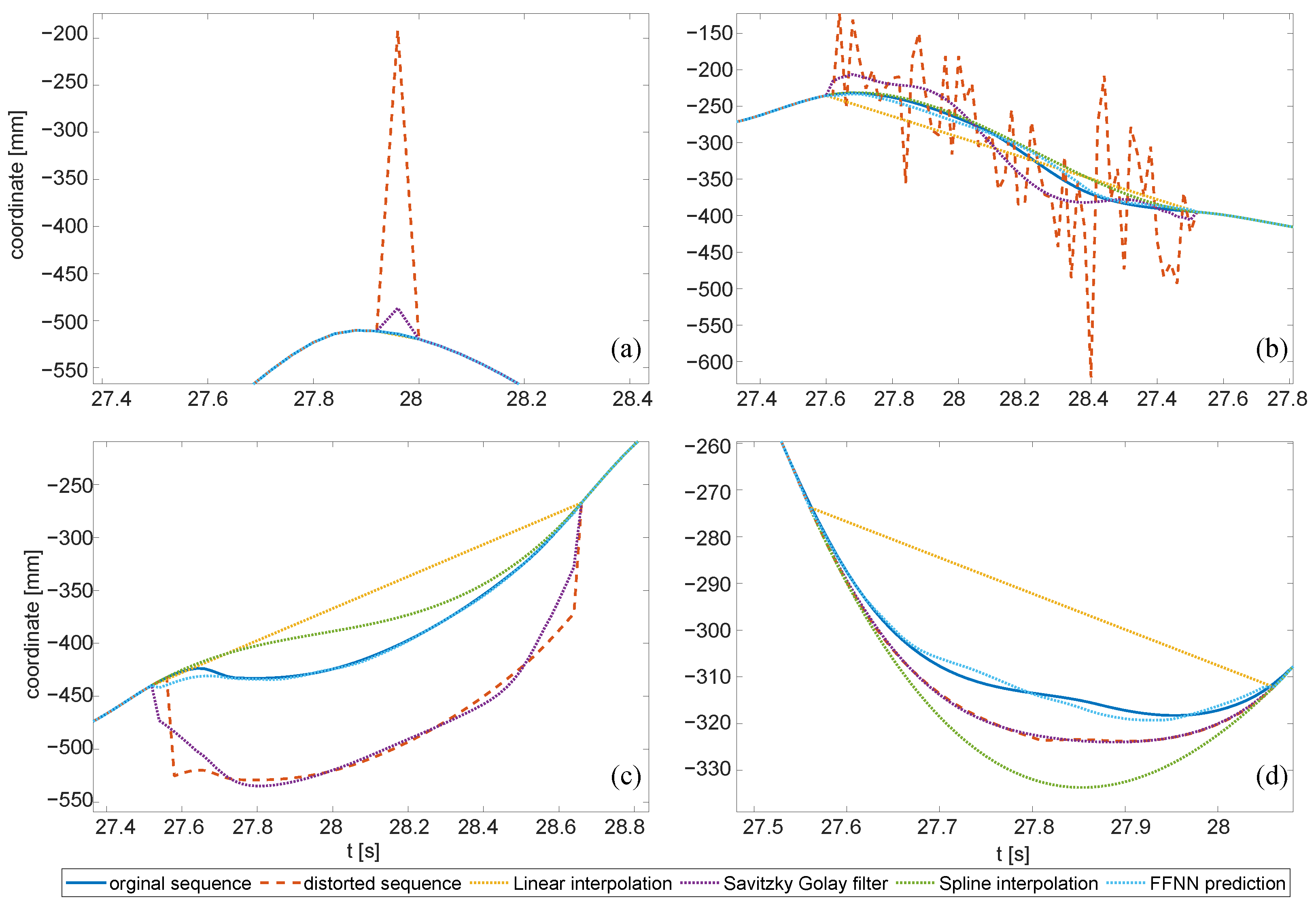
4.2.3. Applicability Testing
- Peak changes were effectively removed with interpolation methods—simple linear or spline (piecewise cubic polynomial); the other two methods in perfect detection would not offer even comparable efficiency, yet in actual classification, they offered just slightly worse performances.
- FFNN offered the best performance for all ‘bulky’ distortions (of longer durations), both hypothetical and classified cases.
- Heavy noise, aside from FFNN, was well cleaned with the Savitzky–Golay filter (see Figure 17b).
- Step changes could be effectively removed with FFNN only.
- Slow changes were the most contradictory—the only appropriate reconstruction method was FFNN; in the case of perfect detection, the efficiency was high, but due to the limited actual detection, the results were quite poor. These results correspond well to the detection of slow changes in E1—low sensitivity and high fall out.
4.3. Results Recap
5. Summary
Author Contributions
Funding
Institutional Review Board Statement
Informed Consent Statement
Data Availability Statement
Acknowledgments
Conflicts of Interest
Abbreviations
| FFNN | feed-forward neural network |
| HF | Hampel filter |
| HML | Human Motion Laboratory |
| LS | least squares |
| M3S | moving three sigma |
| mocap | MOtion CAPture |
| MSE | mean square error |
| NARX-NN | nonlinear autoregressive exogenous neural network |
| NN | neural network |
| PJAIT | Polish–Japanese Academy of Information Technology |
| RMSE | root mean squared error |
References
- Kitagawa, M.; Windsor, B. MoCap for Artists: Workflow and Techniques for Motion Capture; Elsevier/Focal Press: Amsterdam, The Netherlands; Boston, MA, USA, 2008. [Google Scholar]
- Menache, A. Understanding Motion Capture for Computer Animation, 2nd ed.; Morgan Kaufmann: Burlington, MA, USA, 2011. [Google Scholar]
- Mündermann, L.; Corazza, S.; Andriacchi, T.P. The evolution of methods for the capture of human movement leading to markerless motion capture for biomechanical applications. J. Neuroeng. Rehabil. 2006, 3, 6. [Google Scholar] [CrossRef] [PubMed] [Green Version]
- Windolf, M.; Götzen, N.; Morlock, M. Systematic accuracy and precision analysis of video motion capturing systems—Exemplified on the Vicon-460 system. J. Biomech. 2008, 41, 2776–2780. [Google Scholar] [CrossRef] [PubMed]
- Yang, P.F.; Sanno, M.; Brüggemann, G.P.; Rittweger, J. Evaluation of the performance of a motion capture system for small displacement recording and a discussion for its application potential in bone deformation in vivo measurements. Proc. Inst. Mech. Eng. Part H J. Eng. Med. 2012, 226, 838–847. [Google Scholar] [CrossRef] [Green Version]
- Jensenius, A.; Nymoen, K.; Skogstad, S.; Voldsund, A. A Study of the Noise-Level in Two Infrared Marker-Based Motion Capture Systems. In Proceedings of the 9th Sound and Music Computing Conference, SMC 2012, Copenhagen, Denmark, 1–14 July 2012; pp. 258–263. [Google Scholar]
- Eichelberger, P.; Ferraro, M.; Minder, U.; Denton, T.; Blasimann, A.; Krause, F.; Baur, H. Analysis of accuracy in optical motion capture—A protocol for laboratory setup evaluation. J. Biomech. 2016, 49, 2085–2088. [Google Scholar] [CrossRef] [PubMed] [Green Version]
- Skurowski, P.; Pawlyta, M. On the Noise Complexity in an Optical Motion Capture Facility. Sensors 2019, 19, 4435. [Google Scholar] [CrossRef] [PubMed] [Green Version]
- Woltring, H.J. On optimal smoothing and derivative estimation from noisy displacement data in biomechanics. Hum. Mov. Sci. 1985, 4, 229–245. [Google Scholar] [CrossRef]
- Giakas, G.; Baltzopoulos, V. A comparison of automatic filtering techniques applied to biomechanical walking data. J. Biomech. 1997, 30, 847–850. [Google Scholar] [CrossRef]
- Zordan, V.B.; Van Der Horst, N.C. Mapping optical motion capture data to skeletal motion using a physical model. In Proceedings of the 2003 ACM SIGGRAPH/Eurographics Symposium on Computer Animation, San Diego, CA, USA, 26–27 July 2003; Eurographics Association: Goslar, Germany, 2003; pp. 245–250. [Google Scholar]
- Skurowski, P.; Pawlyta, M. Functional Body Mesh Representation, A Simplified Kinematic Model, Its Inference and Applications. Appl. Math. Inf. Sci. 2016, 10, 71–82. [Google Scholar] [CrossRef]
- Barré, A.; Thiran, J.P.; Jolles, B.M.; Theumann, N.; Aminian, K. Soft Tissue Artifact Assessment During Treadmill Walking in Subjects With Total Knee Arthroplasty. IEEE Trans. Biomed. Eng. 2013, 60, 3131–3140. [Google Scholar] [CrossRef]
- Reda, H.E.A.; Benaoumeur, I.; Kamel, B.; Zoubir, A.F. MoCap systems and hand movement reconstruction using cubic spline. In Proceedings of the 2018 5th International Conference on Control, Decision and Information Technologies (CoDIT), Thessaloniki, Greece, 10–13 April 2018; pp. 1–5. [Google Scholar] [CrossRef]
- Tits, M.; Tilmanne, J.; Dutoit, T. Robust and automatic motion-capture data recovery using soft skeleton constraints and model averaging. PLoS ONE 2018, 13, e0199744. [Google Scholar] [CrossRef]
- Camargo, J.; Ramanathan, A.; Csomay-Shanklin, N.; Young, A. Automated gap-filling for marker-based biomechanical motion capture data. Comput. Methods Biomech. Biomed. Eng. 2020, 23, 1180–1189. [Google Scholar] [CrossRef]
- Perepichka, M.; Holden, D.; Mudur, S.P.; Popa, T. Robust Marker Trajectory Repair for MOCAP using Kinematic Reference. In Proceedings of the Motion, Interaction and Games, Newcastle upon Tyne, UK, 28–30 October 2019; Association for Computing Machinery: New York, NY, USA, 2019; pp. 1–10. [Google Scholar] [CrossRef]
- Gløersen, Ø.; Federolf, P. Predicting Missing Marker Trajectories in Human Motion Data Using Marker Intercorrelations. PLoS ONE 2016, 11, e0152616. [Google Scholar] [CrossRef] [PubMed]
- Liu, G.; McMillan, L. Estimation of missing markers in human motion capture. Vis. Comput. 2006, 22, 721–728. [Google Scholar] [CrossRef]
- Kaufmann, M.; Aksan, E.; Song, J.; Pece, F.; Ziegler, R.; Hilliges, O. Convolutional Autoencoders for Human Motion Infilling. arXiv 2020, arXiv:2010.11531. [Google Scholar]
- Zhu, Y. Reconstruction of Missing Markers in Motion Capture Based on Deep Learning. In Proceedings of the 2020 IEEE 3rd International Conference on Information Systems and Computer Aided Education (ICISCAE), Dalian, China, 27–29 September 2020; pp. 346–349. [Google Scholar] [CrossRef]
- Skurowski, P.; Pawlyta, M. Gap Reconstruction in Optical Motion Capture Sequences Using Neural Networks. Sensors 2021, 21, 6115. [Google Scholar] [CrossRef]
- Smolka, J.; Lukasik, E. The rigid body gap filling algorithm. In Proceedings of the 2016 9th International Conference on Human System Interactions (HSI), Portsmouth, UK, 6–8 July 2016; pp. 337–343. [Google Scholar] [CrossRef]
- Royo Sánchez, A.C.; Aguilar Martín, J.J.; Santolaria Mazo, J. Development of a new calibration procedure and its experimental validation applied to a human motion capture system. J. Biomech. Eng. 2014, 136, 124502. [Google Scholar] [CrossRef] [PubMed]
- Nagymáté, G.; Tuchband, T.; Kiss, R.M. A novel validation and calibration method for motion capture systems based on micro-triangulation. J. Biomech. 2018, 74, 16–22. [Google Scholar] [CrossRef] [PubMed]
- Weber, M.; Amor, H.B.; Alexander, T. Identifying Motion Capture Tracking Markers with Self-Organizing Maps. In Proceedings of the 2008 IEEE Virtual Reality Conference, Reno, NV, USA, 8–12 March 2008; pp. 297–298. [Google Scholar] [CrossRef] [Green Version]
- Jiménez Bascones, J.L.; Graña, M.; Lopez-Guede, J.M. Robust labeling of human motion markers in the presence of occlusions. Neurocomputing 2019, 353, 96–105. [Google Scholar] [CrossRef]
- Ghorbani, S.; Etemad, A.; Troje, N.F. Auto-labelling of Markers in Optical Motion Capture by Permutation Learning. In Computer Graphics International Conference; Gavrilova, M., Chang, J., Thalmann, N.M., Hitzer, E., Ishikawa, H., Eds.; Lecture Notes in Computer Science; Springer International Publishing: Cham, Switzerland, 2019; pp. 167–178. [Google Scholar] [CrossRef] [Green Version]
- Han, S.; Liu, B.; Wang, R.; Ye, Y.; Twigg, C.D.; Kin, K. Online optical marker-based hand tracking with deep labels. ACM Trans. Graph. 2018, 37, 166:1–166:10. [Google Scholar] [CrossRef] [Green Version]
- Regression Analysis—Encyclopedia of Mathematics; Springer: Berlin, Germany, 2001.
- Stapor, K. Introduction to Probabilistic and Statistical Methods with Examples in R; Intelligent Systems Reference Library; Springer International Publishing: Cham, Switzerland, 2020. [Google Scholar] [CrossRef]
- Savitzky, A.; Golay, M.J.E. Smoothing and Differentiation of Data by Simplified Least Squares Procedures. Anal. Chem. 1964, 36, 1627–1639. [Google Scholar] [CrossRef]
- Hornik, K. Approximation capabilities of multilayer feedforward networks. Neural Netw. 1991, 4, 251–257. [Google Scholar] [CrossRef]
- Insua, D.R.; Müller, P. Feedforward Neural Networks for Nonparametric Regression. In Practical Nonparametric and Semiparametric Bayesian Statistics; Dey, D., Müller, P., Sinha, D., Eds.; Lecture Notes in Statistics; Springer: New York, NY, USA, 1998; pp. 181–193. [Google Scholar] [CrossRef]
- Czekalski, P.; Łyp, K. Neural network structure optimization in pattern recognition. Stud. Inform. 2014, 35. [Google Scholar] [CrossRef]
- Xu, S.; Lu, B.; Baldea, M.; Edgar, T.F.; Wojsznis, W.; Blevins, T.; Nixon, M. Data cleaning in the process industries. Rev. Chem. Eng. 2015, 31, 453–490. [Google Scholar] [CrossRef]
- Pillai, I.; Fumera, G.; Roli, F. Designing multi-label classifiers that maximize F measures: State of the art. Pattern Recognit. 2017, 61, 394–404. [Google Scholar] [CrossRef] [Green Version]
- Gorodkin, J. Comparing two K-category assignments by a K-category correlation coefficient. Comput. Biol. Chem. 2004, 28, 367–374. [Google Scholar] [CrossRef] [PubMed]


| No. | Name | Scenario | Duration | Difficulty |
|---|---|---|---|---|
| 1 | Static | Actor stands in the T-pose in the middle of the scene, looks around, and shifts from one foot to another | 22 s | easy, static |
| 2 | Sitting | Actor stands in the middle of the scene and then sits on a chair; actor stands again after a few seconds and repeats this three times | 29 s | occlusions |
| Operator | Seq. No | Recording | Errors Identified by | Error Verification | |||
|---|---|---|---|---|---|---|---|
| Human | Algorithm | Approved | Rejected | Missed | |||
| None | 2 | Sitting | — | 29 | 16 | 13 | 4 |
| Expert | 2 | Sitting | 20 | 9 | 0 | 0 | 0 |
| Intermediate | 2 | Sitting | 18 | 11 | 2 | 9 | 0 |
| Beginner 1 | 2 | Sitting | 10 | 37 | 20 | 17 | 2 |
| Beginner 2 | 2 | Sitting | 11 | 46 | 26 | 20 | 1 |
| Peaks | Heavy Noise | Step Change | Slow Change | |
|---|---|---|---|---|
| Distorted | 0.19065 | 0.17717 | 0.18069 | 0.10129 |
| Linear interpolation (perfect) | 0.00136 | 0.18322 | 0.15939 | 0.18795 |
| Linear interpolation (classified) | 0.03947 | 0.18514 | 0.15623 | 0.29339 |
| Savitzky–Golay filter (perfect) | 0.01900 | 0.04963 | 0.17440 | 0.10130 |
| Savitzky–Golay filter (classified) | 0.08159 | 0.06855 | 0.17553 | 0.10173 |
| Spline interpolation (perfect) | 0.00025 | 0.11041 | 0.09780 | 0.10972 |
| Spline interpolation (classified) | 0.03429 | 0.68692 | 0.10895 | 0.19935 |
| FFNN predictor (perfect) | 0.01841 | 0.01953 | 0.01933 | 0.01875 |
| FFNN predictor (classified) | 0.03944 | 0.04547 | 0.04409 | 0.11000 |
| Peaks | Heavy Noise | Step Change | Slow Change | |
|---|---|---|---|---|
| Distorted | 0.26906 | 0.26340 | 0.26282 | 0.15037 |
| Linear interpolation (perfect) | 0.00186 | 0.25487 | 0.28409 | 0.27662 |
| Linear interpolation (classified) | 0.05144 | 0.26360 | 0.27618 | 0.38908 |
| Savitzky–Golay filter (perfect) | 0.02678 | 0.07211 | 0.25361 | 0.15046 |
| Savitzky–Golay filter (classified) | 0.08959 | 0.08895 | 0.25510 | 0.15083 |
| Spline interpolation (perfect) | 0.00039 | 0.14679 | 0.15207 | 0.15955 |
| Spline interpolation (classified) | 0.04754 | 0.95512 | 0.16358 | 0.23918 |
| FFNN predictor (perfect) | 0.02785 | 0.02468 | 0.02581 | 0.02612 |
| FFNN predictor (classified) | 0.05537 | 0.05201 | 0.06349 | 0.14717 |
| Peaks | Heavy Noise | Step Change | Slow Change | |
|---|---|---|---|---|
| Distorted | 0.38228 | 0.39623 | 0.39247 | 0.21676 |
| Linear interpolation (perfect) | 0.00273 | 0.44107 | 0.44015 | 0.39172 |
| Linear interpolation (classified) | 0.07007 | 0.45679 | 0.45630 | 0.55692 |
| Savitzky–Golay filter (perfect) | 0.03880 | 0.11228 | 0.37892 | 0.21704 |
| Savitzky–Golay filter (classified) | 0.10383 | 0.16007 | 0.38120 | 0.21748 |
| Spline interpolation (perfect) | 0.00058 | 0.24337 | 0.28188 | 0.25274 |
| Spline interpolation (classified) | 0.06753 | 1.58979 | 0.37534 | 0.35679 |
| FFNN predictor (perfect) | 0.04169 | 0.03711 | 0.03972 | 0.03735 |
| FFNN predictor (classified) | 0.07903 | 0.11433 | 0.10284 | 0.20549 |
Publisher’s Note: MDPI stays neutral with regard to jurisdictional claims in published maps and institutional affiliations. |
© 2022 by the authors. Licensee MDPI, Basel, Switzerland. This article is an open access article distributed under the terms and conditions of the Creative Commons Attribution (CC BY) license (https://creativecommons.org/licenses/by/4.0/).
Share and Cite
Skurowski, P.; Pawlyta, M. Detection and Classification of Artifact Distortions in Optical Motion Capture Sequences. Sensors 2022, 22, 4076. https://doi.org/10.3390/s22114076
Skurowski P, Pawlyta M. Detection and Classification of Artifact Distortions in Optical Motion Capture Sequences. Sensors. 2022; 22(11):4076. https://doi.org/10.3390/s22114076
Chicago/Turabian StyleSkurowski, Przemysław, and Magdalena Pawlyta. 2022. "Detection and Classification of Artifact Distortions in Optical Motion Capture Sequences" Sensors 22, no. 11: 4076. https://doi.org/10.3390/s22114076
APA StyleSkurowski, P., & Pawlyta, M. (2022). Detection and Classification of Artifact Distortions in Optical Motion Capture Sequences. Sensors, 22(11), 4076. https://doi.org/10.3390/s22114076