
Structural Damage Identification Based on Transmissibility in Time Domain


Abstract
:1. Introduction
2. Transmissibility of Strain in Time Domain Based on Empirical Mode Decomposition
3. Finite Element Model Updating Based on Modal Response Transmissibility
3.1. Establishment of Objective Function
3.2. Establishment of Discrepancy Vectors
3.3. Establishment of Sensitivity Matrix
4. Numerical Example
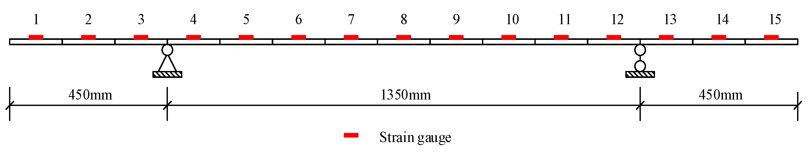
4.1. The Model of Simply Supported Overhanging Beam
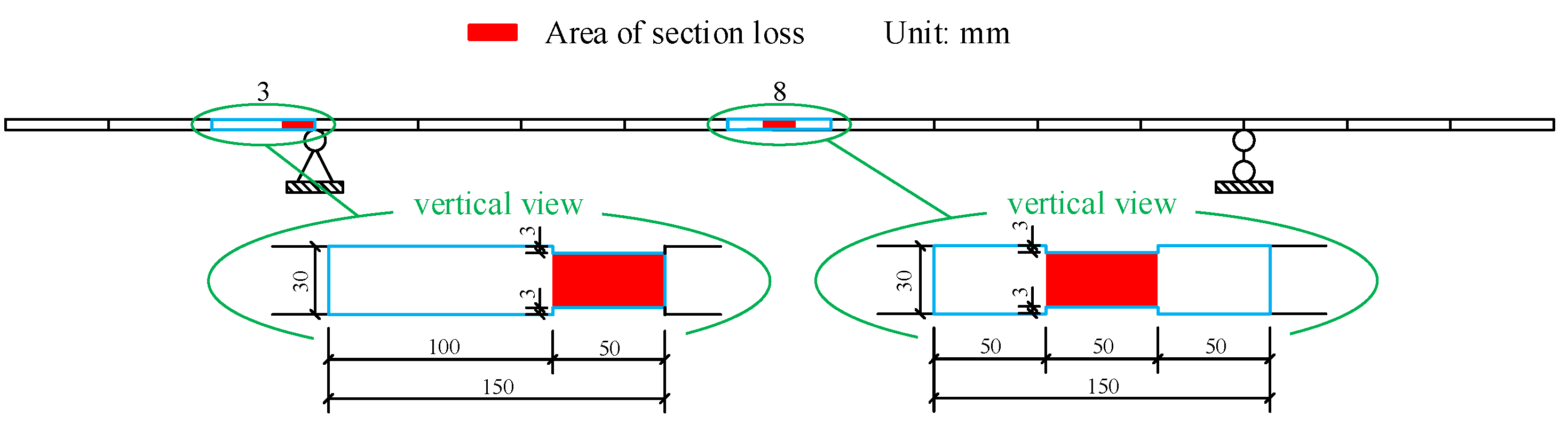
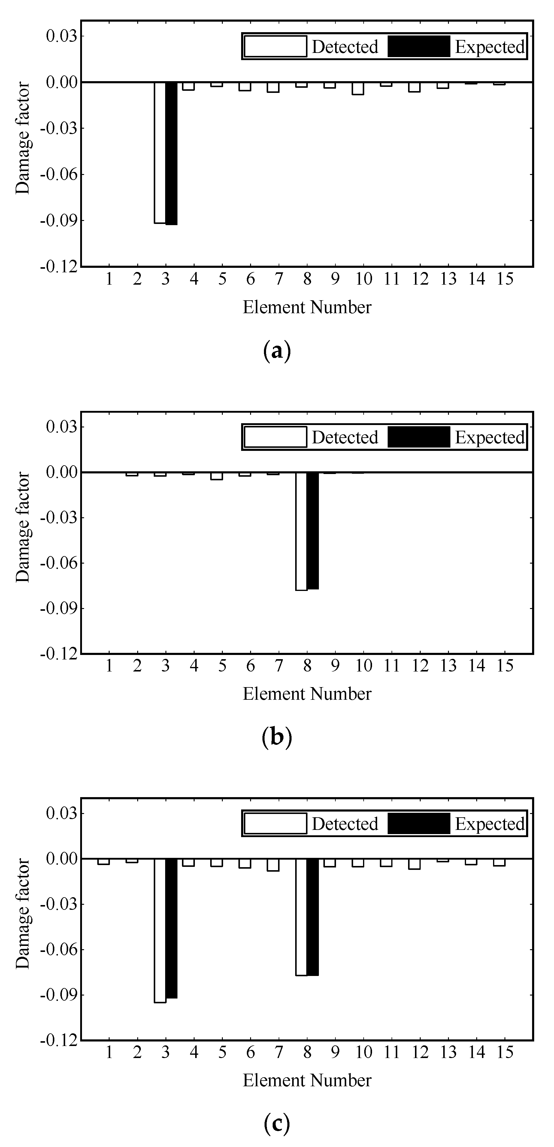
4.2. Damage Scenario Simulation
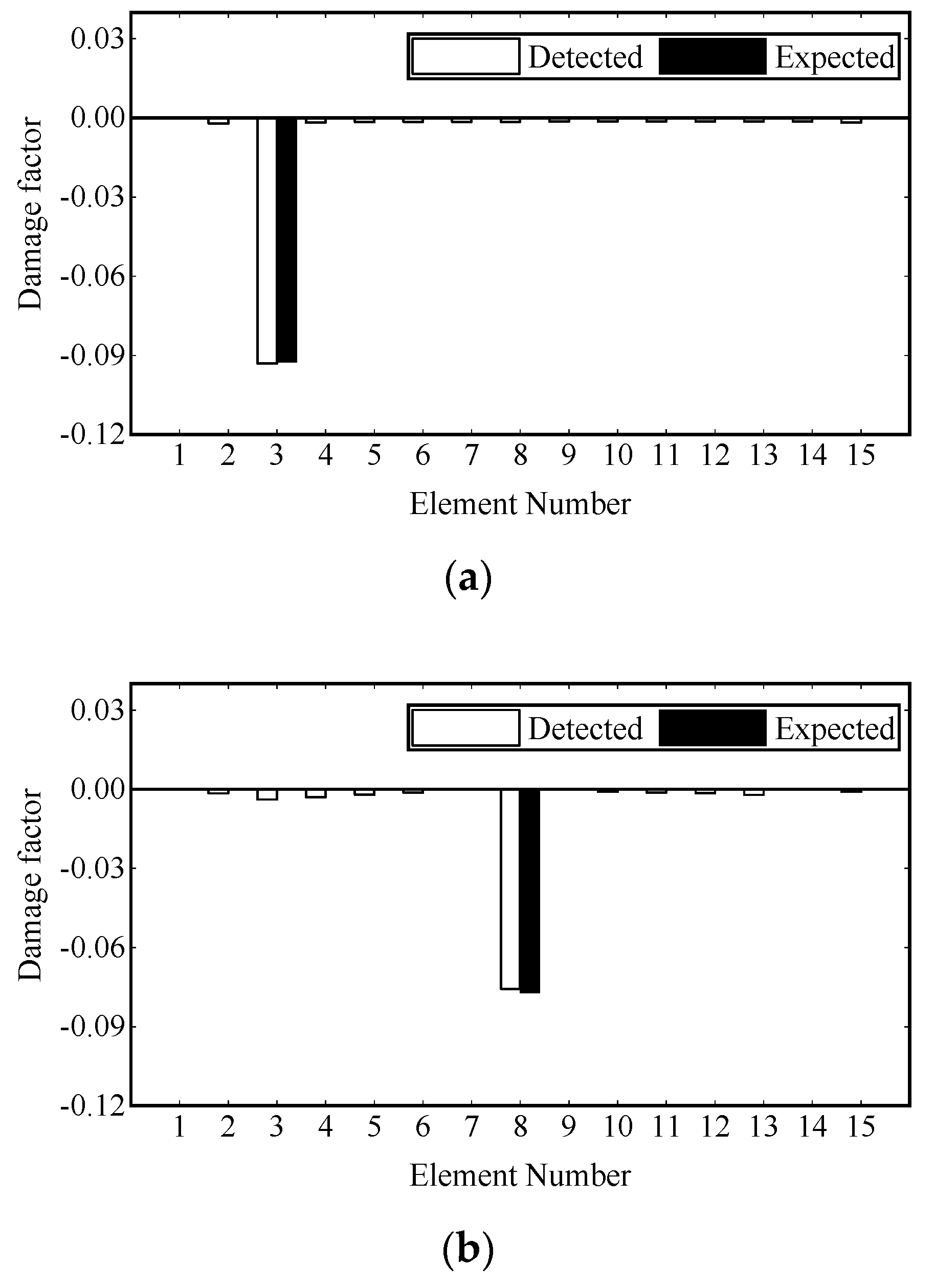
4.3. Damage Identification Based on Transmissibility in Time Domain
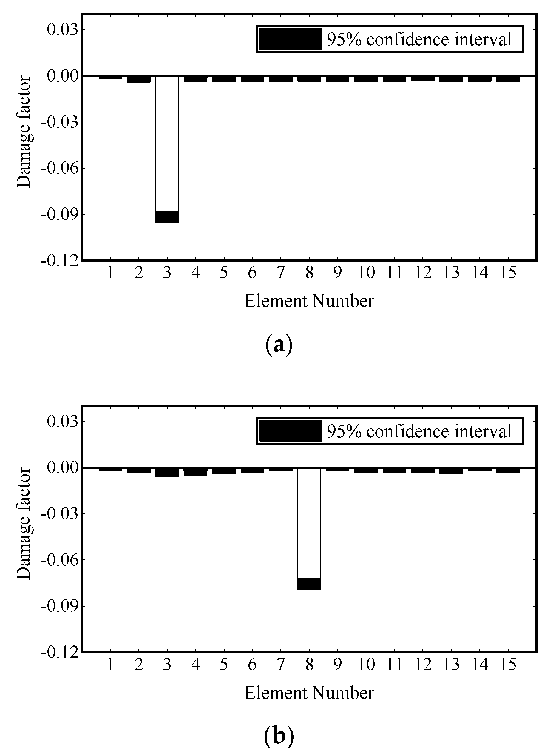
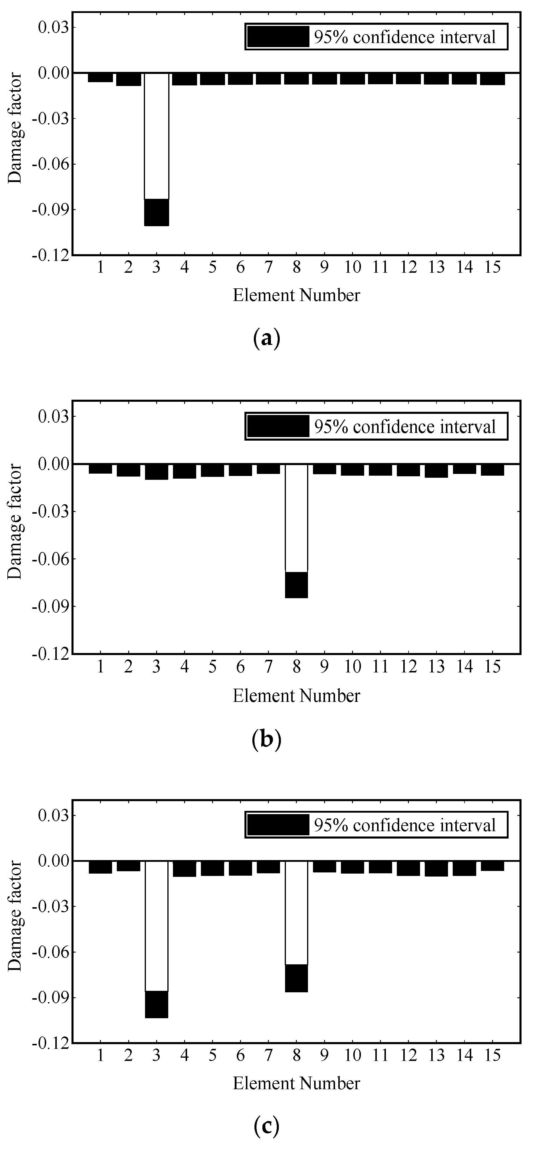
4.4. Influence of Noise on Damage Identification
5. Experimental Investigation
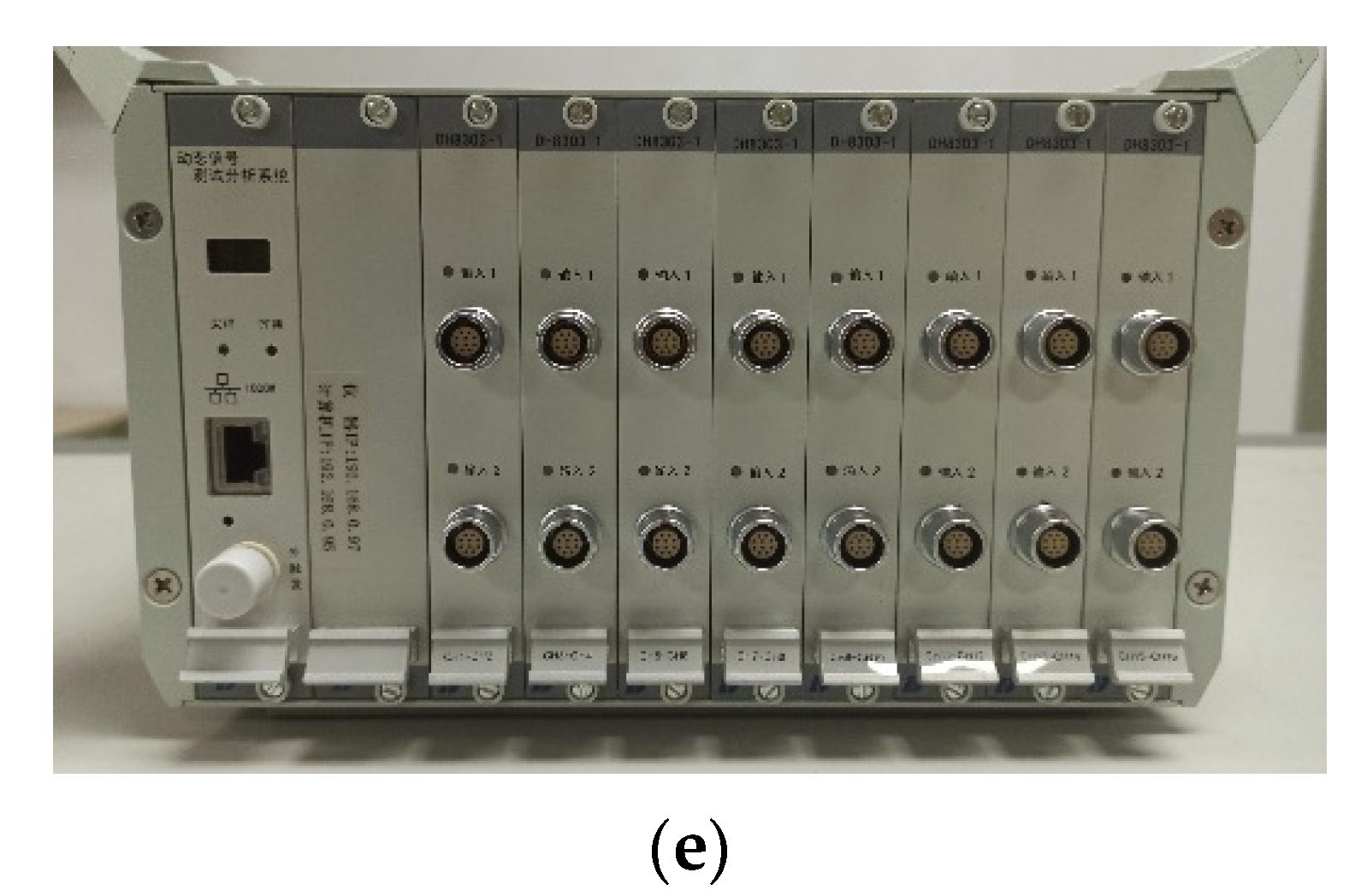
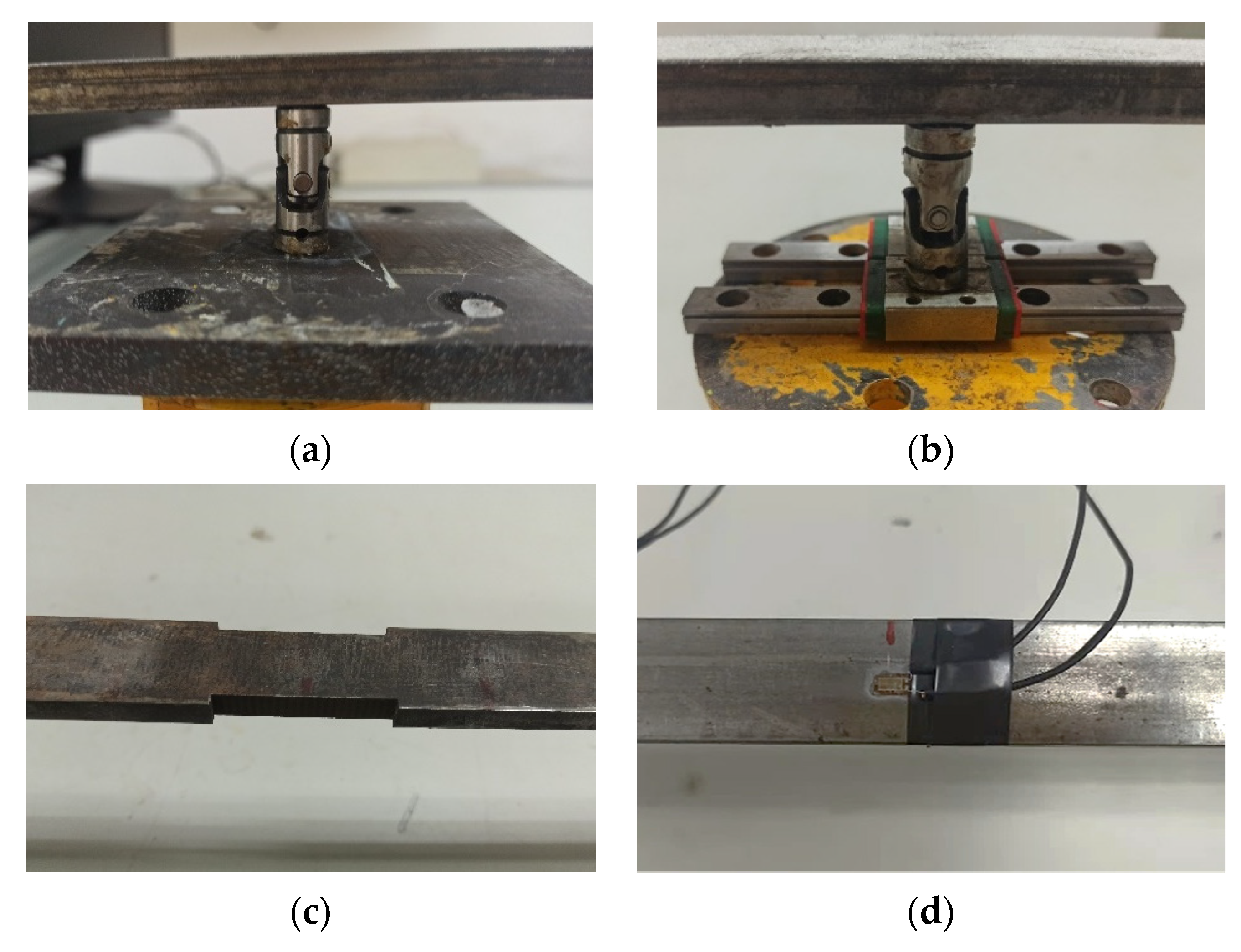
5.1. Experimental Setup
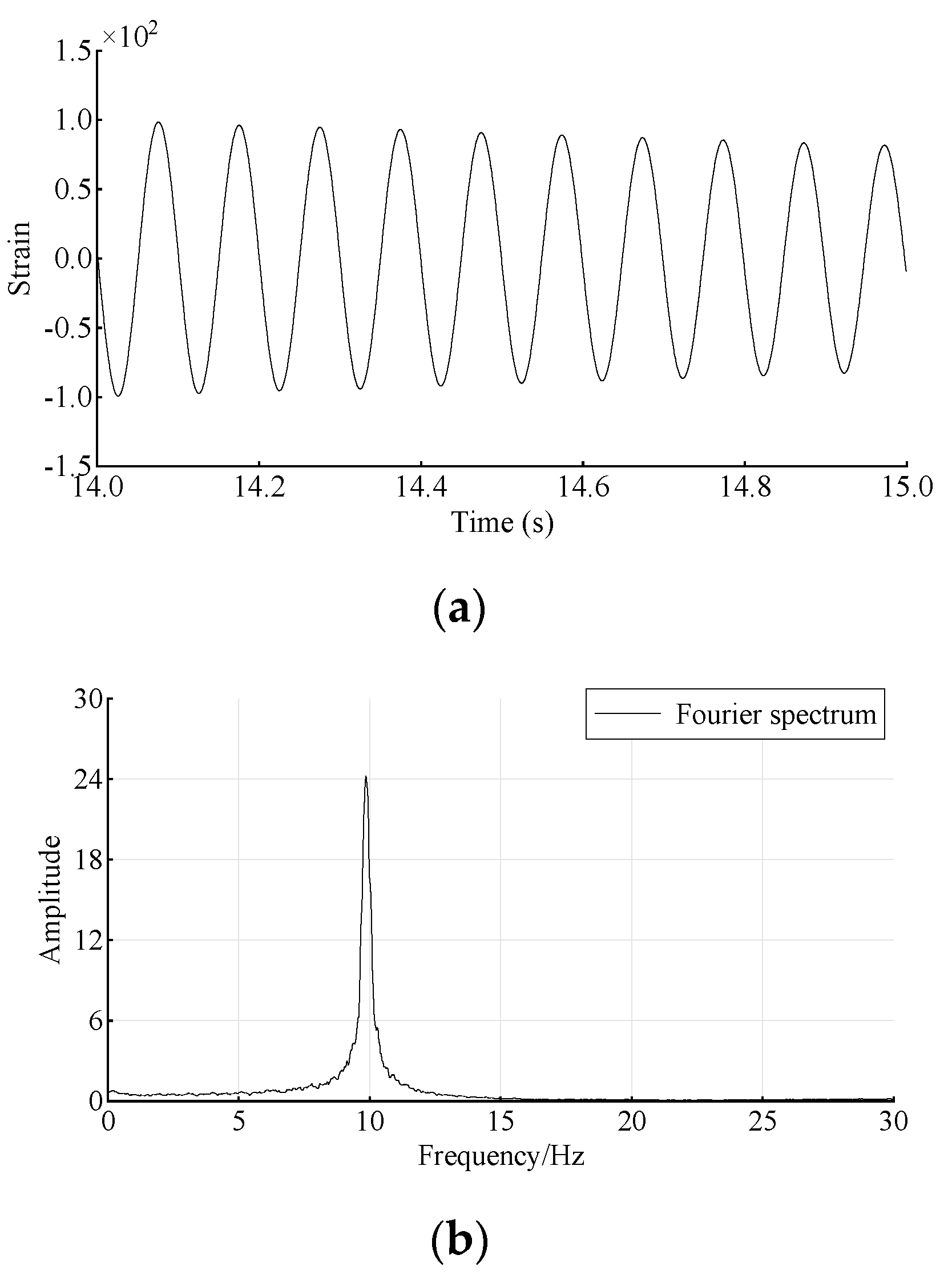
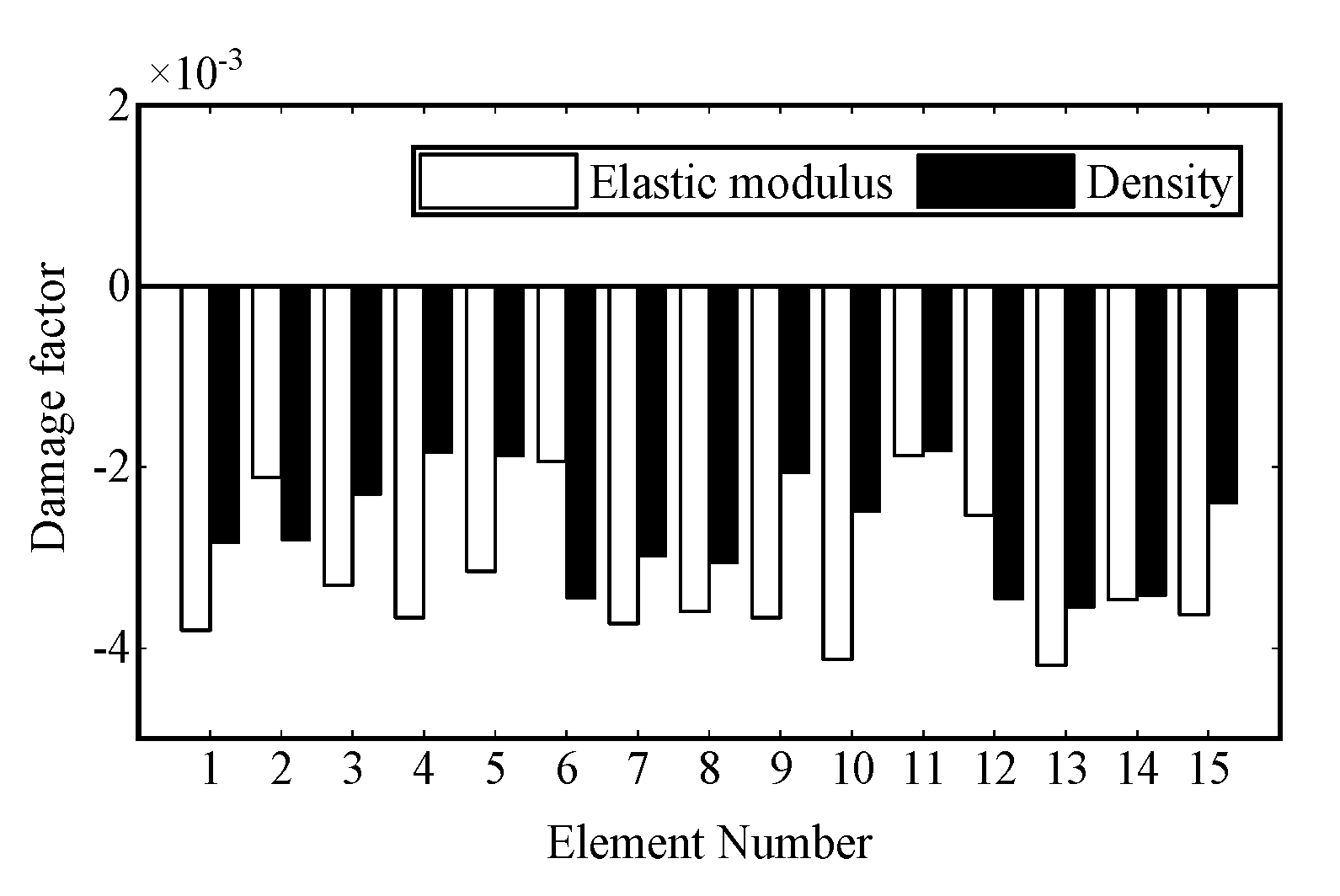
5.2. Accuracy Detection of FE Model
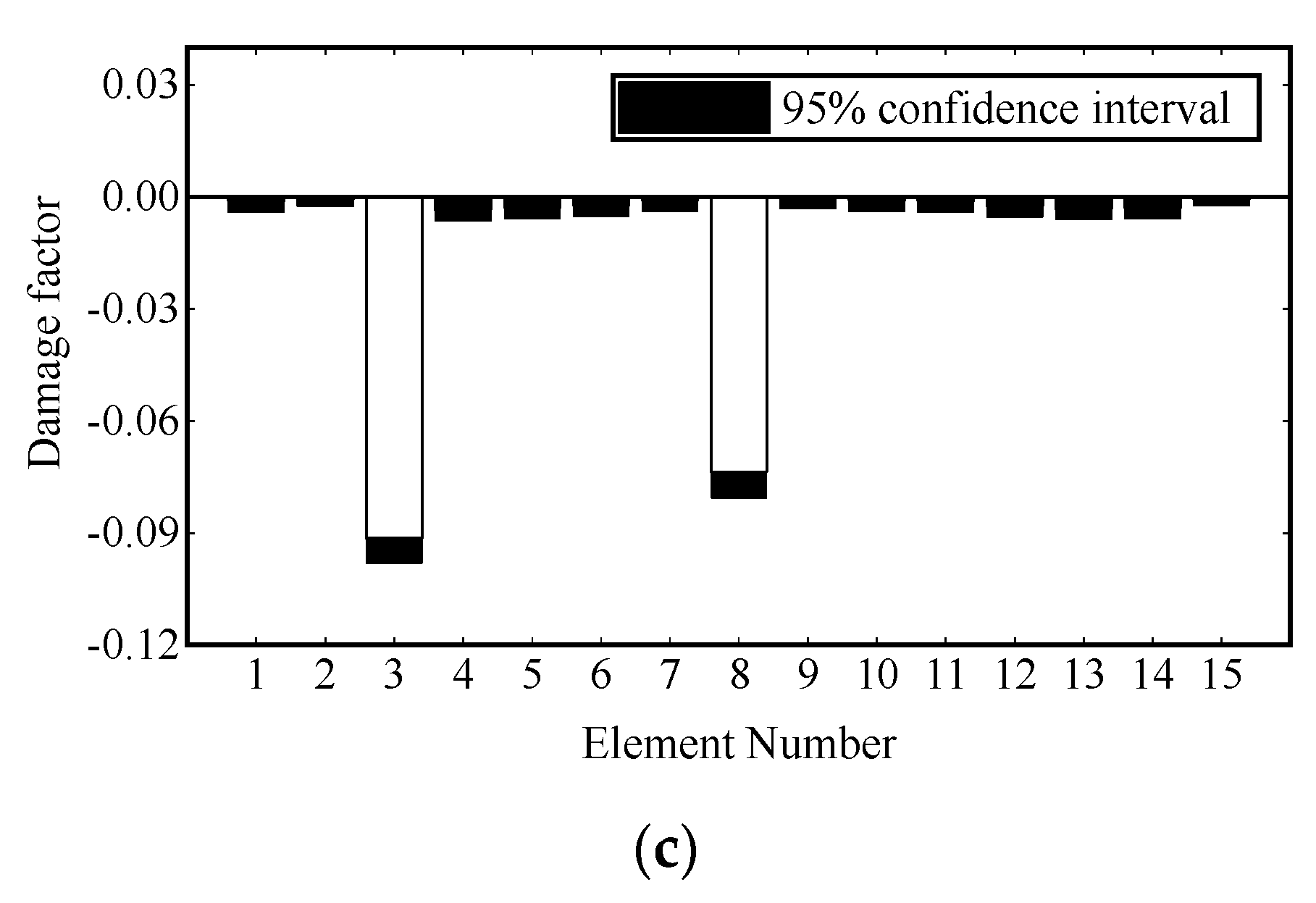
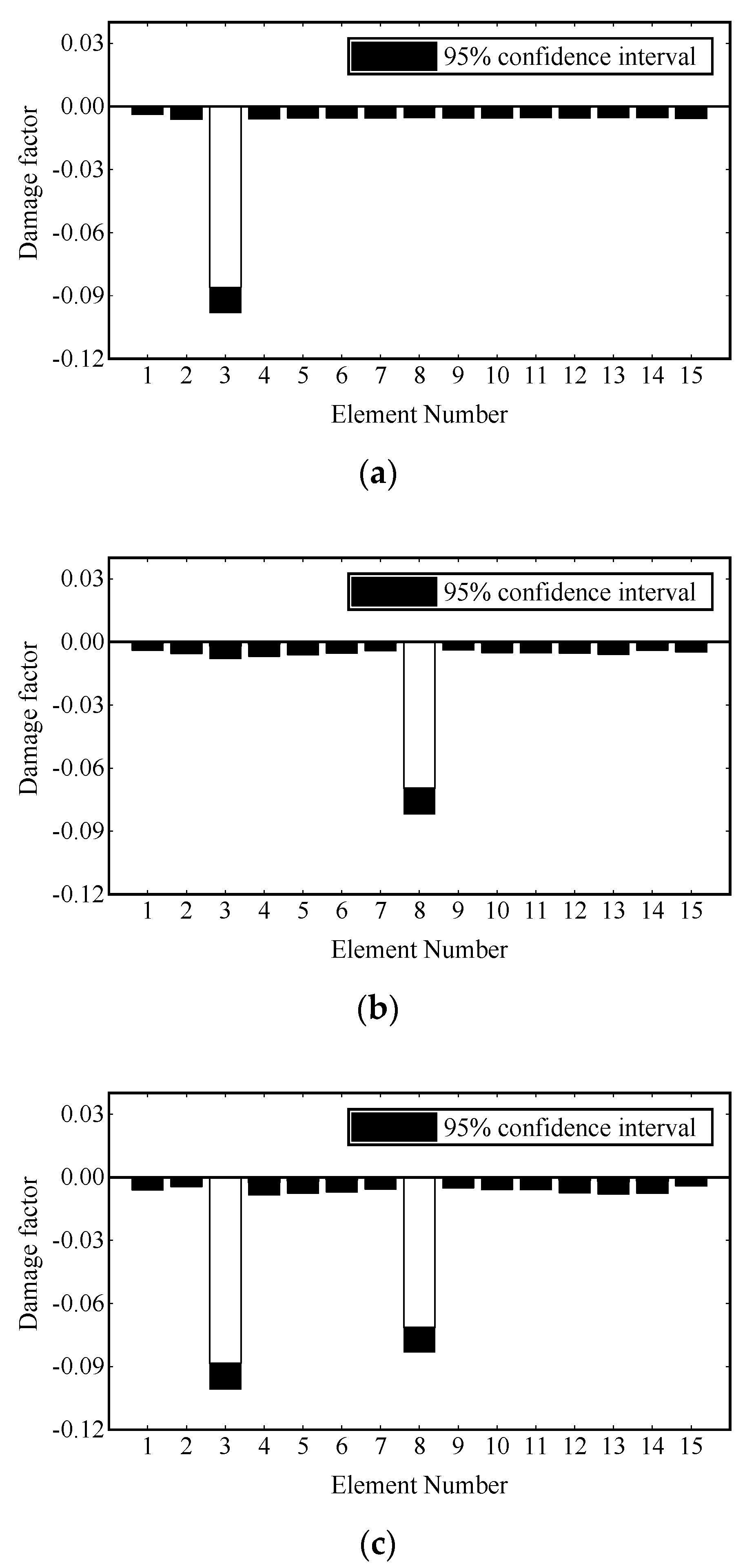
5.3. Damage Identification
6. Conclusions
- (1)
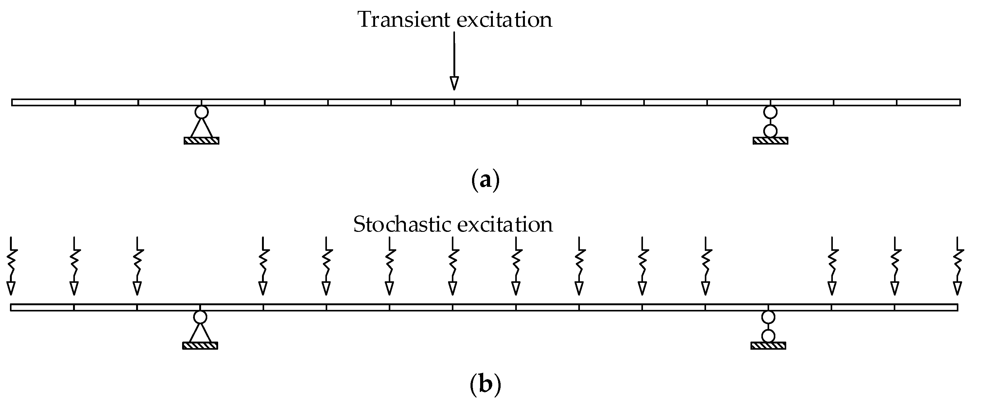
- In this study, a novel strategy of damage identification in the time domain is proposed. Compared with the existing damage identification method, the proposed method uses the internal relationship between two locations in the structure as the basis of damage identification. The damage identification can be located and quantified in the time domain without modal identification and frequent time–frequency conversion, which can greatly improve efficiency on the premise of ensuring accuracy. It is suitable to identify the structural damage under transient excitation or stochastic excitation that can excite the modal response of the structure.
- (2)
- According to numerical analysis results, the accuracy of damage identification under different noise levels and excitation types can be guaranteed. Although the recognition accuracy will be affected under a high noise level, it can still accurately locate the damaged element. The proposed method has good noise resistance and robustness.
- (3)
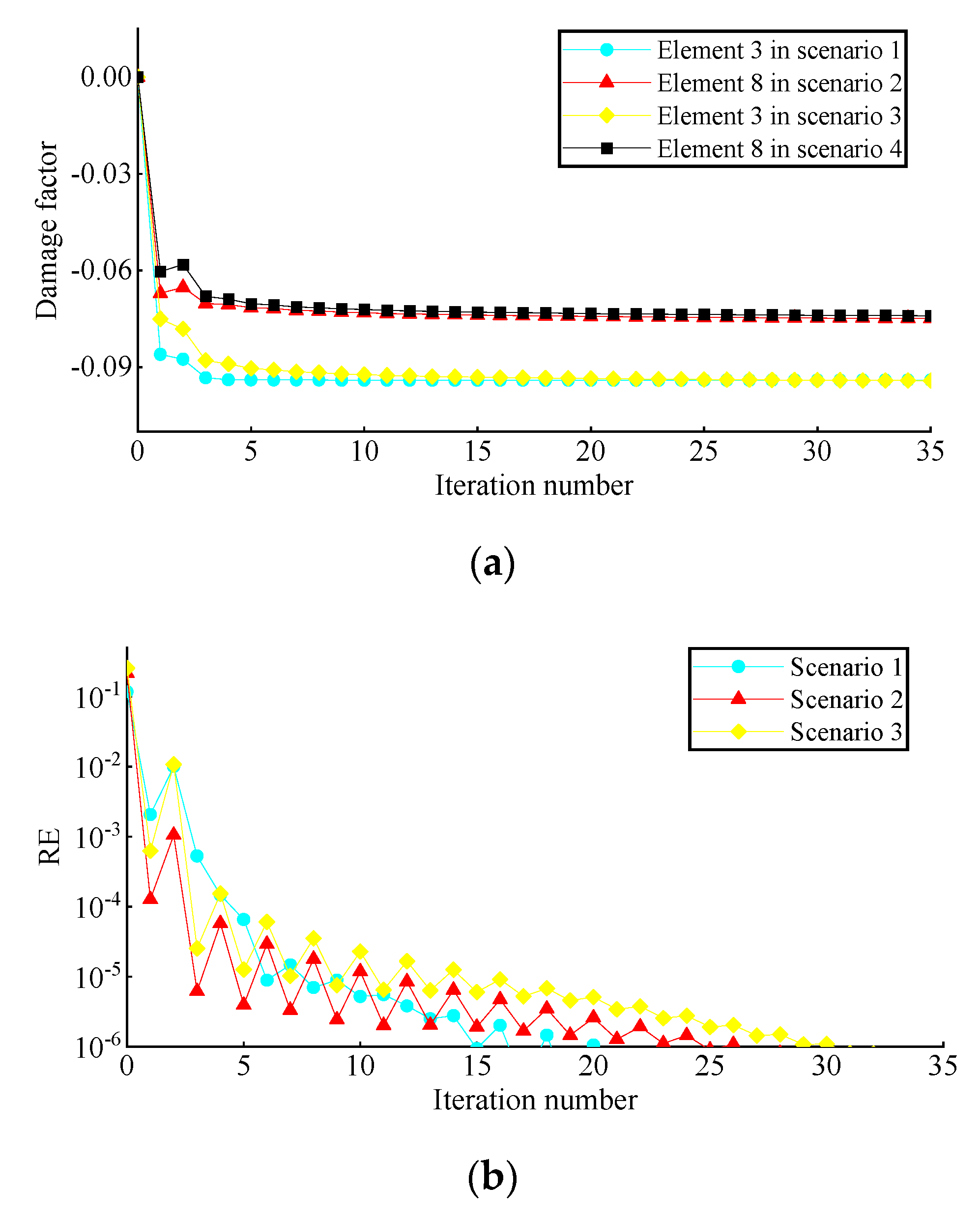
- The experimental beam corresponding to the simulation case verifies the effectiveness and accuracy of the damage identification method. Under the three damage scenarios, the damage factors converge stably and rapidly.
Author Contributions
Funding
Institutional Review Board Statement
Informed Consent Statement
Data Availability Statement
Acknowledgments
Conflicts of Interest
Nomenclature
| n | number of damage parameters | Abbreviation | |
| Nt | number of time points | FE | finite element |
| Nr | number of transmissibility | RE | relative error |
| ε | strain response vector | DOF | degree of freedom |
| Q | modal coordinate vector | EMD | empirical mode decomposition |
| the i-th modal response vector | Superscripts or subscripts | ||
| K, M | stiffness matrix, mass matrix | T | transpose of matrix or vector |
| B | strain-displacement matrix | a, b | location index |
| J | objective function | j | the j-th mode |
| Frobenius norm | (l) | the l-th element | |
| , Λ | the s-th eigenvalue, eigenvalue matrix | k | the k-th iteration |
| W | weighting matrix | r | reconstructed modal response |
| S | sensitivity matrix | f | modes of FE model |
| αl, α | damage factor of l-th element, damage factor vector | m | modal response extracted from measured response |
| ψ, Ψ | strain modal contribution, strain modal matrix | d | modes and modal response of actual structure |
References
- Aulakh, D.S.; Bhalla, S. 3D torsional experimental strain modal analysis for structural health monitoring using piezoelectric sensors. Measurement 2021, 180, 109476. [Google Scholar] [CrossRef]
- Chang, C.M.; Lin, T.K.; Chang, C.W. Applications of neural network models for structural health monitoring based on derived modal properties. Measurement 2018, 129, 457–470. [Google Scholar] [CrossRef]
- Nokhbatolfoghahai, A.; Navazi, H.M.; Groves, R.M. Evaluation of the sparse reconstruction and the delay-and-sum damage imaging methods for structural health monitoring under different environmental and operational conditions. Measurement 2021, 169, 108495. [Google Scholar] [CrossRef]
- Salehi, H.; Chakrabartty, S.; Biswas, S.; Burgueno, R. Localized damage identification in plate-like structures using self-powered sensor data: A pattern recognition strategy. Measurement 2019, 135, 23–38. [Google Scholar] [CrossRef]
- Zhang, H.L.; Wu, Z.F.; Shum, P.P.; Dinh, X.Q.; Low, C.W.; Xu, Z.L.; Wang, R.X.; Shao, X.G.; Fu, S.N.; Tong, W.J.; et al. Highly sensitive strain sensor based on helical structure combined with Mach-Zehnder interferometer in multicore fiber. Sci. Rep.-Uk 2017, 7, srep46633. [Google Scholar] [CrossRef] [Green Version]
- Lakshmi, K.; Rao, A.R.M.; Gopalakrishnan, N. Singular spectrum analysis combined with ARMAX model for structural damage detection. Struct. Control Health Monit. 2017, 24, e1960. [Google Scholar] [CrossRef]
- Figueiredo, E.; Figueiras, J.; Park, G.; Farrar, C.R.; Worden, K. Influence of the Autoregressive Model Order on Damage Detection. Comput. -Aided Civ. Infrastruct. Eng. 2011, 26, 225–238. [Google Scholar] [CrossRef]
- Yao, R.; Pakzad, S.N. Autoregressive statistical pattern recognition algorithms for damage detection in civil structures. Mech. Syst. Signal Process. 2012, 31, 355–368. [Google Scholar] [CrossRef]
- Shahidi, S.G.; Nigro, M.B.; Pakzad, S.N.; Pan, Y. Structural damage detection and localisation using multivariate regression models and two-sample control statistics. Struct. Infrastruct. Eng. 2014, 11, 1277–1293. [Google Scholar] [CrossRef]
- Abdeljaber, O.; Avci, O.; Kiranyaz, S.; Gabbouj, M.; Inman, D.J. Real-time vibration-based structural damage detection using one-dimensional convolutional neural networks. J. Sound Vib. 2017, 388, 154–170. [Google Scholar] [CrossRef]
- Neves, A.C.; González, I.; Leander, J.; Karoumi, R. Structural health monitoring of bridges: A model-free ANN-based approach to damage detection. J. Civ. Struct. Health Monit. 2017, 7, 689–702. [Google Scholar] [CrossRef] [Green Version]
- Ruffels, A.; Gonzalez, I.; Karoumi, R. Model-free damage detection of a laboratory bridge using artificial neural networks. J. Civ. Struct. Health Monit. 2020, 10, 183–195. [Google Scholar] [CrossRef]
- Bao, Y.; Tang, Z.; Li, H.; Zhang, Y. Computer vision and deep learning–based data anomaly detection method for structural health monitoring. Struct. Health Monit. 2018, 18, 401–421. [Google Scholar] [CrossRef]
- Katunin, A. Identification of structural damage using S-transform from 1D and 2D mode shapes. Measurement 2021, 173, 108656. [Google Scholar] [CrossRef]
- Mousavi, M.; Holloway, D.; Olivier, J.C.; Gandomi, A.H. Beam damage detection using synchronisation of peaks in instantaneous frequency and amplitude of vibration data. Measurement 2021, 168, 108297. [Google Scholar] [CrossRef]
- Sabz, A.; Reddy, J.N.; Jiao, P.C.; Alavi, A.H. Structural damage detection using rate of total energy. Measurement 2019, 133, 91–98. [Google Scholar] [CrossRef]
- Shu, Y.J.; Wu, J.; Zhou, S.L.; Wang, J.J.; Wang, W.S. Pile damage identification method for high-pile wharfs based on axial static strain distribution. Measurement 2021, 180, 109607. [Google Scholar] [CrossRef]
- Umar, S.; Bakhary, N.; Abidin, A.R.Z. Response surface methodology for damage detection using frequency and mode shape. Measurement 2018, 115, 258–268. [Google Scholar] [CrossRef]
- Ma, K.; Wu, J.; Li, H.; Ye, F. Damage identification of bridge structure based on frequency domain decomposition and strain mode. J. Vibroeng. 2019, 21, 2096–2105. [Google Scholar] [CrossRef]
- Pérez, M.A.; Font-Moré, J.; Fernández-Esmerats, J. Structural damage assessment in lattice towers based on a novel frequency domain-based correlation approach. Eng. Struct. 2021, 226, 111329. [Google Scholar] [CrossRef]
- Sepe, V.; Capecchi, D.; De Angelis, M. Modal model identification of structures under unmeasured seismic excitations. Earthq. Eng. Struct. Dyn. 2005, 34, 807–824. [Google Scholar] [CrossRef]
- Gesualdo, A.; Fortunato, A.; Penta, F.; Monaco, M. Structural identification of tall buildings: A reinforced concrete structure as a case study. Case Stud. Constr. Mater. 2021, 15, e00701. [Google Scholar] [CrossRef]
- Jian, G.; Yong, C.; Bing-nan, S. Experimental study of structural damage identification based on WPT and coupling NN. J. Zhejiang Univ.-Sci. A 2005, 6, 663–669. [Google Scholar] [CrossRef]
- Cui, H.; Xu, X.; Peng, W.; Zhou, Z.; Hong, M. A damage detection method based on strain modes for structures under ambient excitation. Measurement 2018, 125, 438–446. [Google Scholar] [CrossRef]
- Cancelli, A.; Laflamme, S.; Alipour, A.; Sritharan, S.; Ubertini, F. Vibration-based damage localization and quantification in a pretensioned concrete girder using stochastic subspace identification and particle swarm model updating. Struct. Health Monit. 2019, 19, 587–605. [Google Scholar] [CrossRef]
- Zhang, C.-D.; Xu, Y.-L. Multi-level damage identification with response reconstruction. Mech. Syst. Signal Process. 2017, 95, 42–57. [Google Scholar] [CrossRef]
- Pan, C.; Yu, L. Sparse regularization-based damage detection in a bridge subjected to unknown moving forces. J. Civ. Struct. Health Monit. 2019, 9, 425–438. [Google Scholar] [CrossRef]
- He, J.J.; Zhou, Y.B.; Guan, X.F.; Zhang, W.; Zhang, W.F.; Liu, Y.M. Time Domain Strain/Stress Reconstruction Based on Empirical Mode Decomposition: Numerical Study and Experimental Validation. Sensors 2016, 16, 1290. [Google Scholar] [CrossRef] [Green Version]
- He, J.J.; Guan, X.F.; Liu, Y.M. Structural response reconstruction based on empirical mode decomposition in time domain. Mech. Syst. Signal Process. 2012, 28, 348–366. [Google Scholar] [CrossRef]
- Wan, Z.; Li, S.; Huang, Q.; Wang, T. Structural response reconstruction based on the modal superposition method in the presence of closely spaced modes. Mech. Syst. Signal Process. 2014, 42, 14–30. [Google Scholar] [CrossRef]
- Reumers, P.; Van Hoorickx, C.; Schevenels, M.; Lombaert, G. Density filtering regularization of finite element model updating problems. Mech. Syst. Signal Process. 2019, 128, 282–294. [Google Scholar] [CrossRef]
- Girardi, M.; Padovani, C.; Pellegrini, D.; Robol, L. A finite element model updating method based on global optimization. Mech. Syst. Signal Process. 2021, 152, 107372. [Google Scholar] [CrossRef]
- Zhang, J.Z.K. Comparative studies on structural damage detection using Lp norm regularisation. E3S Web Conf. 2020, 143, 171–186. [Google Scholar]
- Jin, W.M.; Yang, Q.W.; Shen, X.; Lu, F.J. Damage Identification for Truss Structures Using Eigenvectors. Adv. Mater. Res.-Switz. 2013, 753–755, 2351–2355. [Google Scholar] [CrossRef]
- Xu, Z.D.; Wu, K.Y. Damage Detection for Space Truss Structures Based on Strain Mode under Ambient Excitation. J. Eng. Mech. 2012, 138, 1215–1223. [Google Scholar] [CrossRef]
- Li, X.Y.; Law, S.S. Adaptive Tikhonov regularization for damage detection based on nonlinear model updating. Mech. Syst. Signal Process. 2010, 24, 1646–1664. [Google Scholar] [CrossRef]


| Damage Scenario | Damage Description |
|---|---|
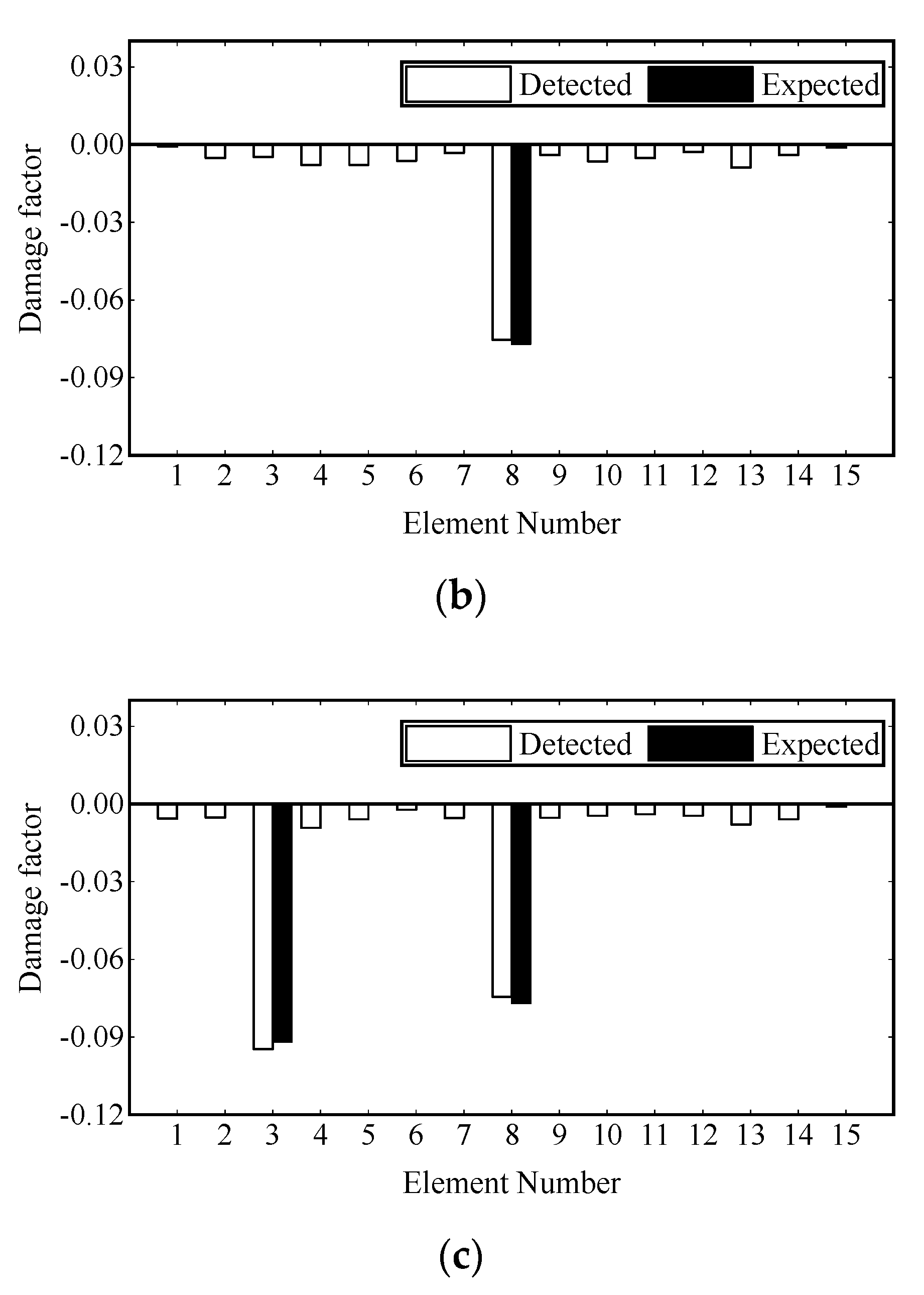
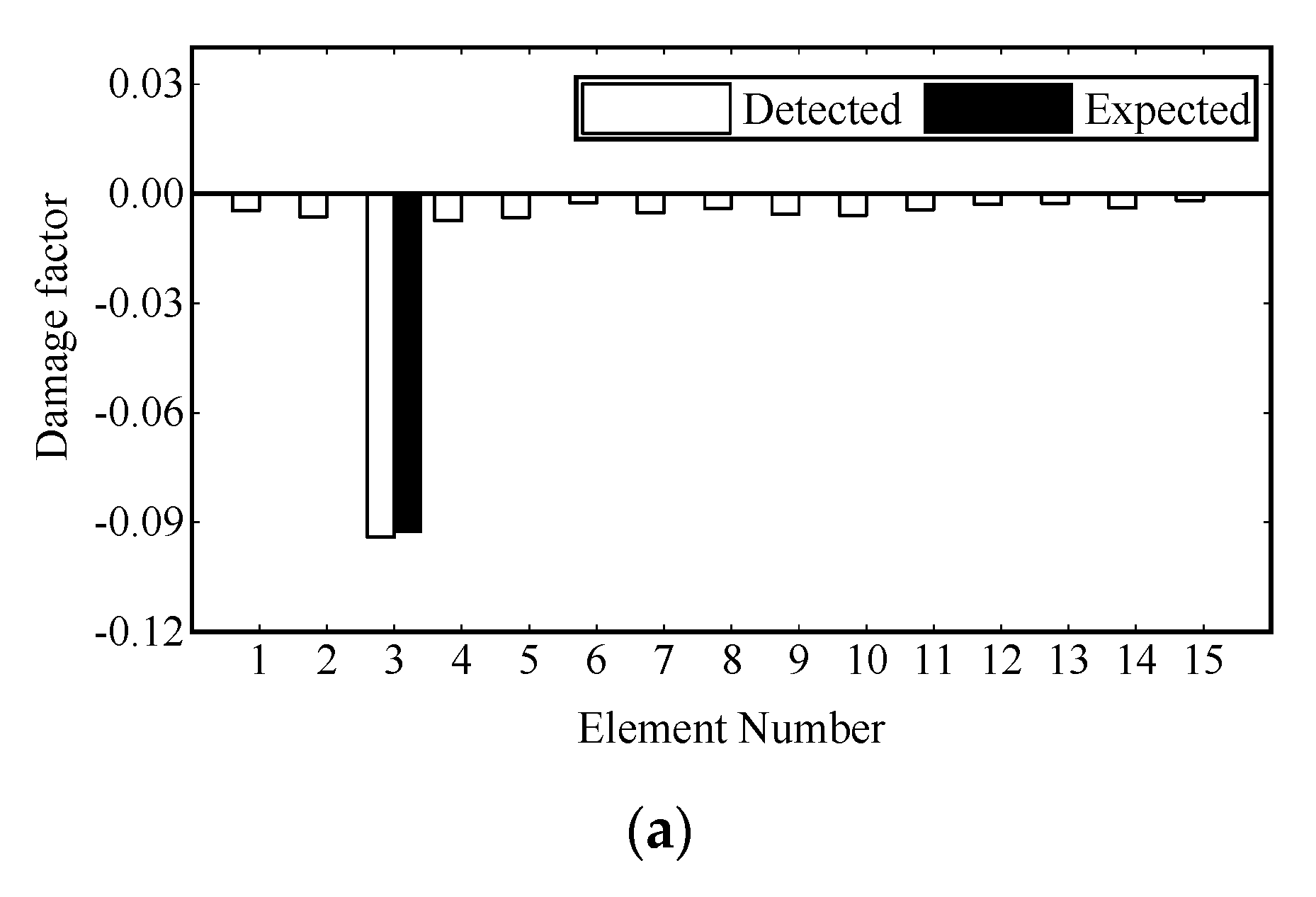
| Scenario 1 | Section loss of Element 3 |
| Scenario 2 | Section loss of Element 8 |
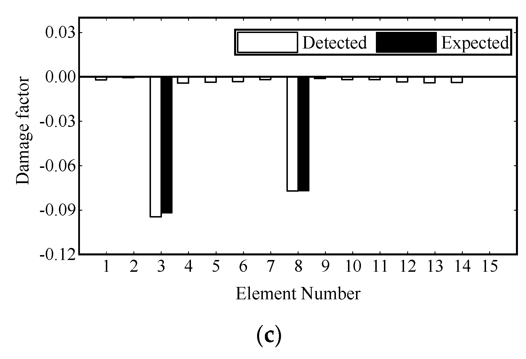
| Scenario 3 | Section loss of Element 3 and Element 8 |
| Calculated Method | Scenario 1 | Scenario 2 | Scenario 3 | |
|---|---|---|---|---|
| Element number | 3 | 8 | 3 | 8 |
| Calculated value | −0.0926 | −0.0771 | −0.0920 | −0.0771 |
| Properties | Value |
|---|---|
| Type | BF350-3AA strain gauge |
| Resistance (Ω) | 349.8 ± 0.1 |
| Sensitivity coefficient | 2.1 ± 0.1 |
| Substrate size | 7.1 mm × 4.5 mm |
| Grid size | 5.0 mm × 3.0 mm |
| Grid material | Constantan |
| Limited strain | 2.0% |
| Damage Scenario | Scenario 1 | Scenario 2 | Scenario 3 |
|---|---|---|---|
| Number of iterations | 21 | 27 | 31 |
| Time consumption (s) | 0.476 | 0.597 | 0.657 |
Publisher’s Note: MDPI stays neutral with regard to jurisdictional claims in published maps and institutional affiliations. |
© 2022 by the authors. Licensee MDPI, Basel, Switzerland. This article is an open access article distributed under the terms and conditions of the Creative Commons Attribution (CC BY) license (https://creativecommons.org/licenses/by/4.0/).
Share and Cite
Zou, Y.; Lu, X.; Yang, J.; Wang, T.; He, X. Structural Damage Identification Based on Transmissibility in Time Domain. Sensors 2022, 22, 393. https://doi.org/10.3390/s22010393
Zou Y, Lu X, Yang J, Wang T, He X. Structural Damage Identification Based on Transmissibility in Time Domain. Sensors. 2022; 22(1):393. https://doi.org/10.3390/s22010393
Chicago/Turabian StyleZou, Yunfeng, Xuandong Lu, Jinsong Yang, Tiantian Wang, and Xuhui He. 2022. "Structural Damage Identification Based on Transmissibility in Time Domain" Sensors 22, no. 1: 393. https://doi.org/10.3390/s22010393
APA StyleZou, Y., Lu, X., Yang, J., Wang, T., & He, X. (2022). Structural Damage Identification Based on Transmissibility in Time Domain. Sensors, 22(1), 393. https://doi.org/10.3390/s22010393