
Clustering by Errors: A Self-Organized Multitask Learning Method for Acoustic Scene Classification

Abstract
:1. Introduction
- (1)
- To the best of our knowledge, we are the first to automatically construct a taxonomy for acoustic scenes by learning similarity relationships from classification errors.
- (2)
- By incorporating the constructed two-level class hierarchy, the proposed self-organized multitask learning method improves the performance of ASC.
2. Related Works
3. Proposed Method
3.1. Overview
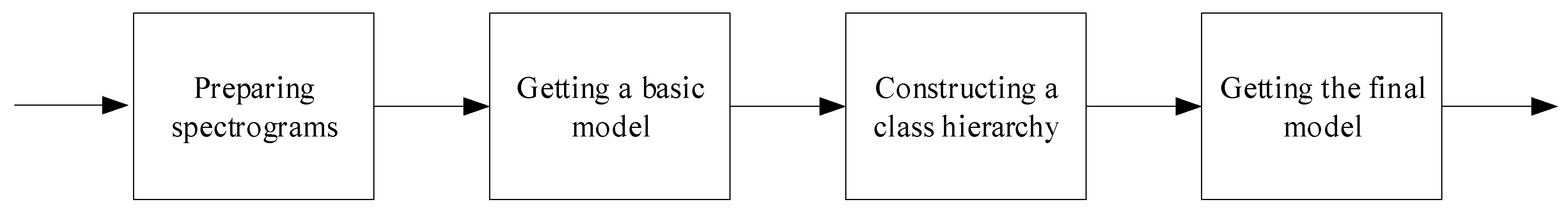
- (1)
- Preparing spectrograms: transforming the raw audio segments into spectrograms that are suitable for CNN models.
- (2)
- Getting a basic model: training a single-task CNN model as a basic model using the spectrograms and original fine-grained scene labels.
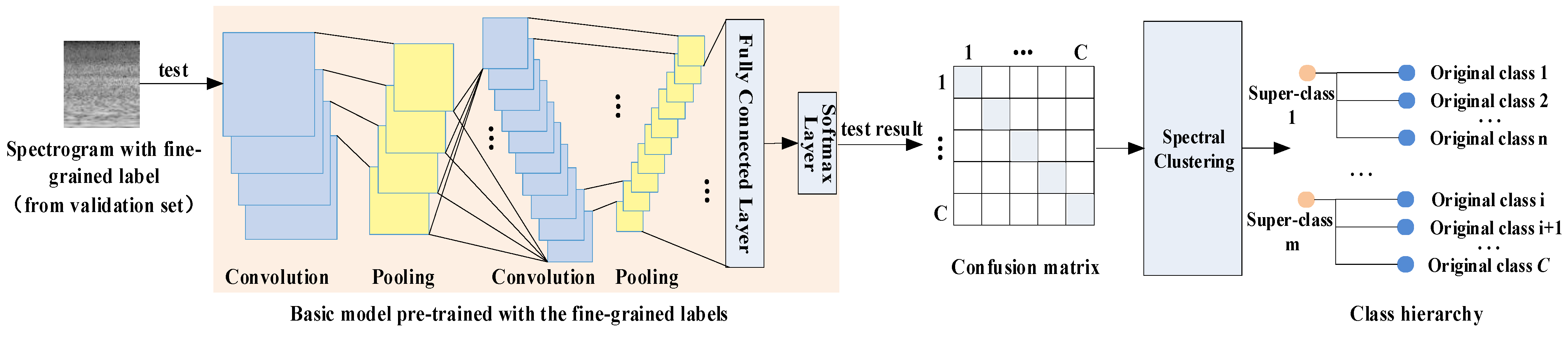
- (3)
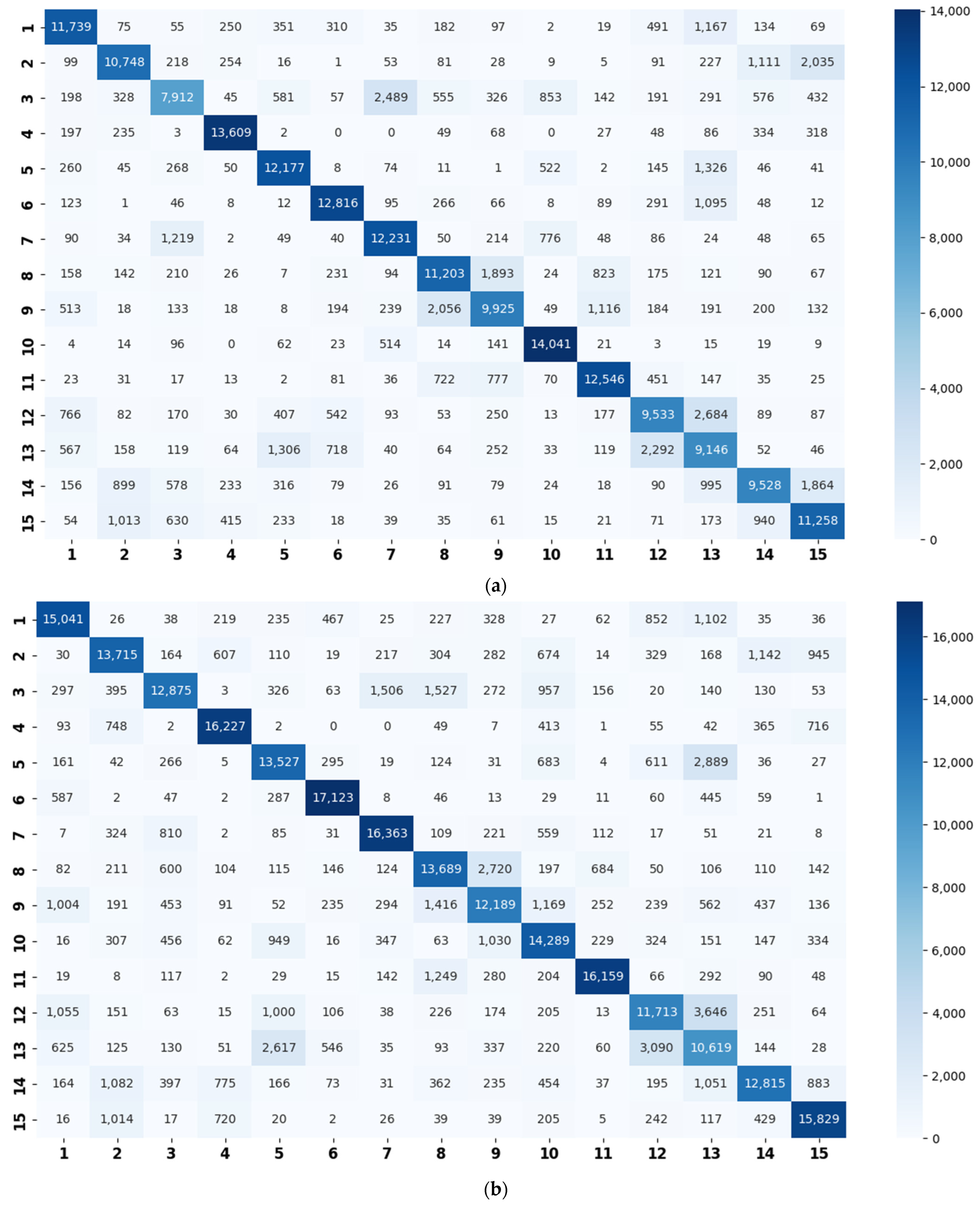
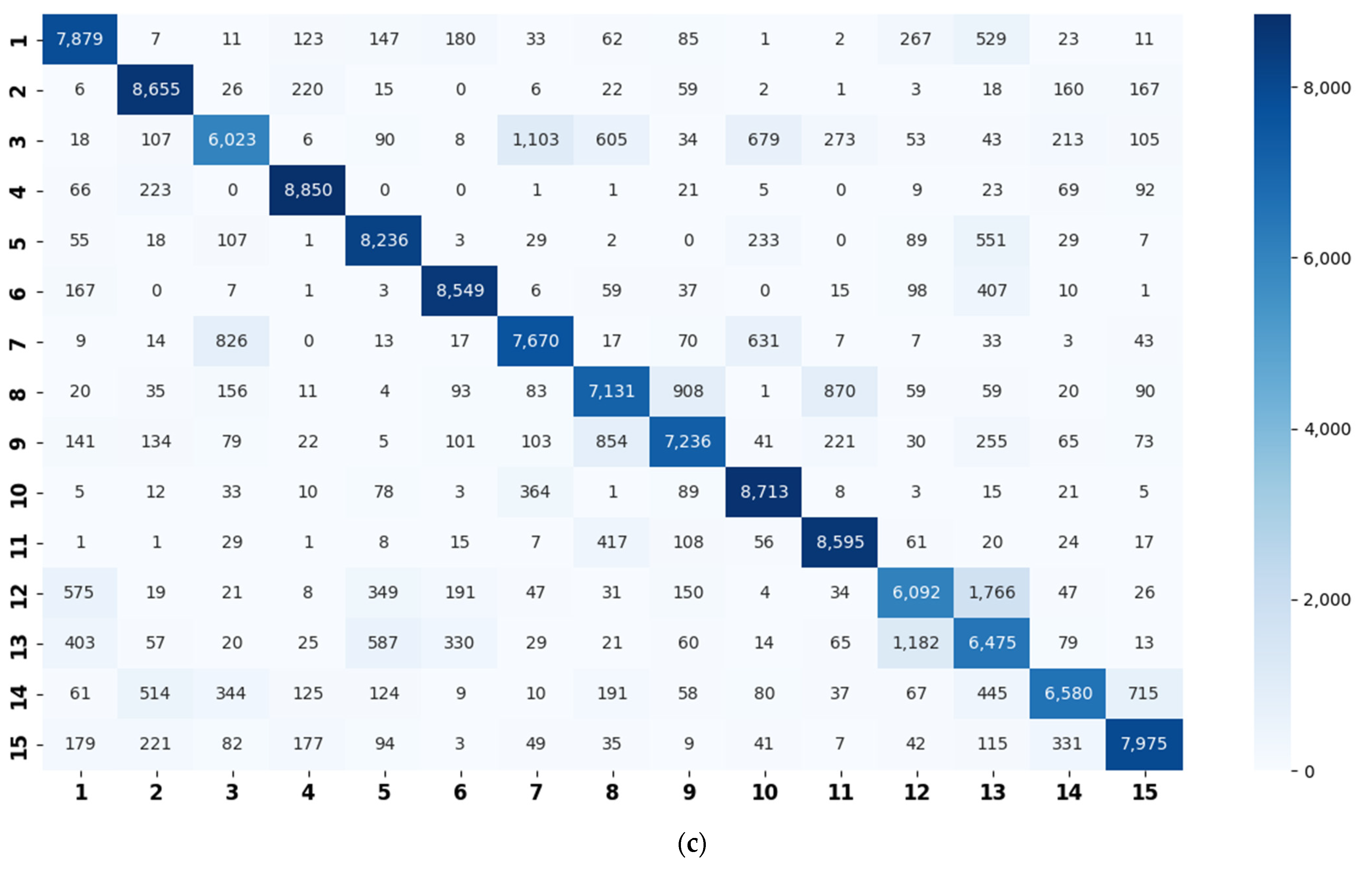
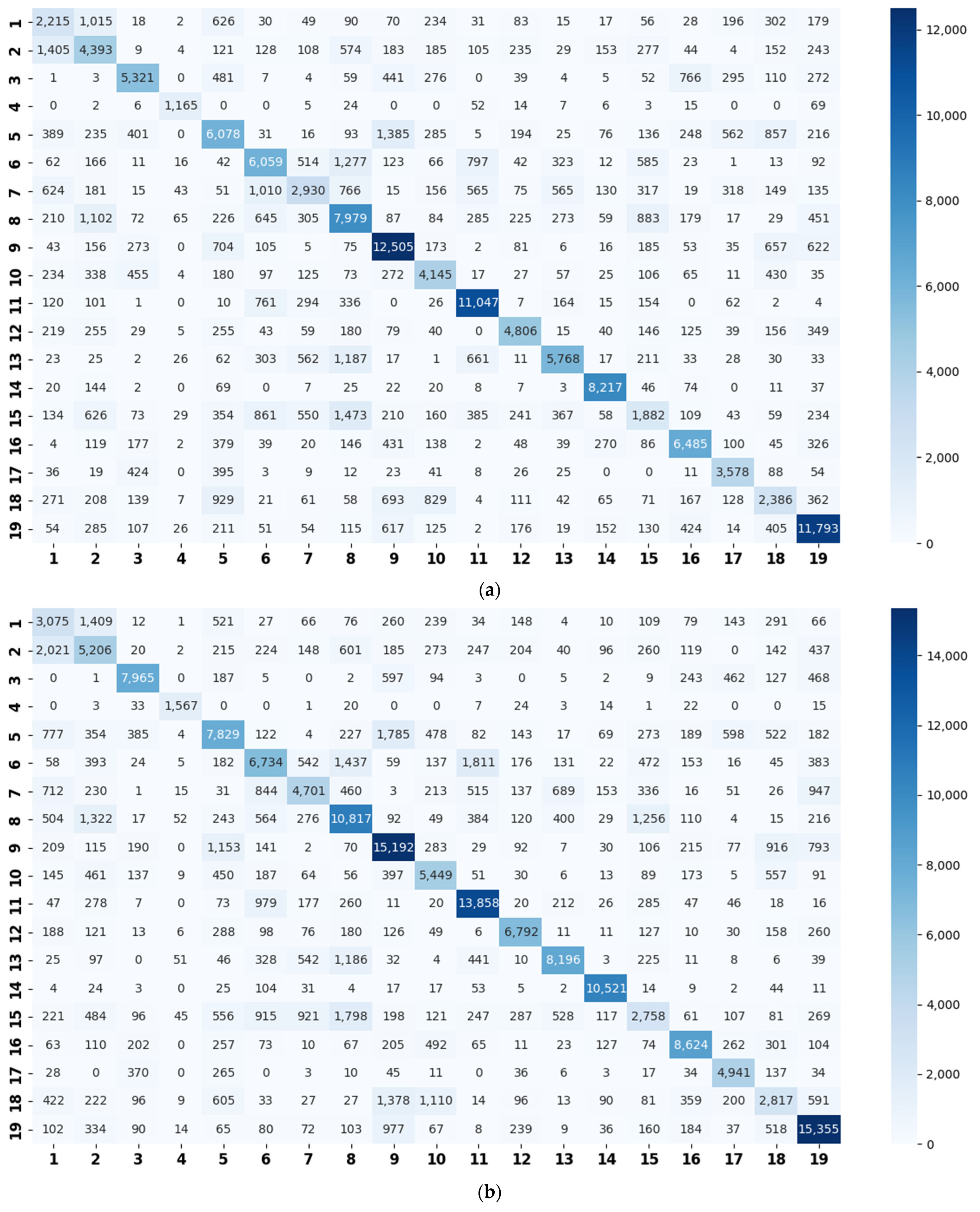
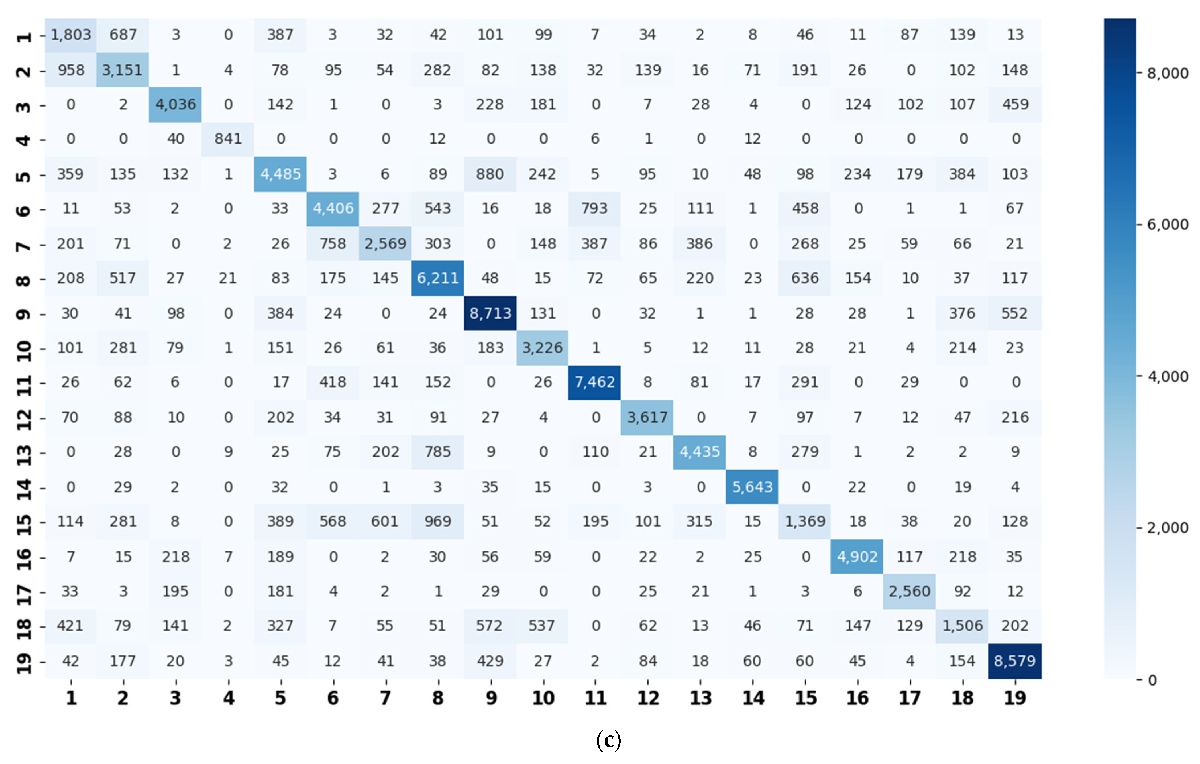
- Constructing a class hierarchy: testing the validation set on the basic model to obtain a confusion matrix. The spectral clustering is performed on the confusion matrix to generate super-classes.
- (4)
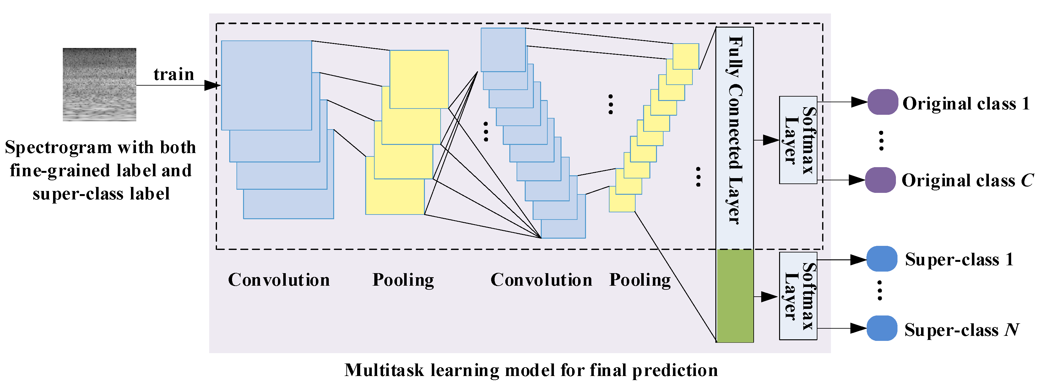
- Getting the final model: training a multitask CNN model as the final classifier to predict both the original scene class and the constructed super-class using hierarchical labels.
3.2. Spectrograms Generation
3.3. Basic Model
3.4. Super-Class Labels Construction
| Algorithm 1. Clustering algorithm in super-class generation |
| Input: the confusion matrix, number of clusters . Output: super-class clusters 1. Set the diagonal elements of to zero: 2. Normalize each row of F by the following equations: , 3. Transform into a symmetric matrix D: 4. Assume that is a diagonal matrix whose elements are set as: , 5. Construct the Laplacian matrix by: 6. Calculate the eigenvectors corresponding to the N smallest eigenvalues of . 7. Let be the matrix containing as columns; let be the -th row of . 8. Use K-means algorithm to cluster into N clusters . 9. Output clusters with ,. |
3.5. Multitask Learning Model
4. Experiments and Results
4.1. Experiment Setup
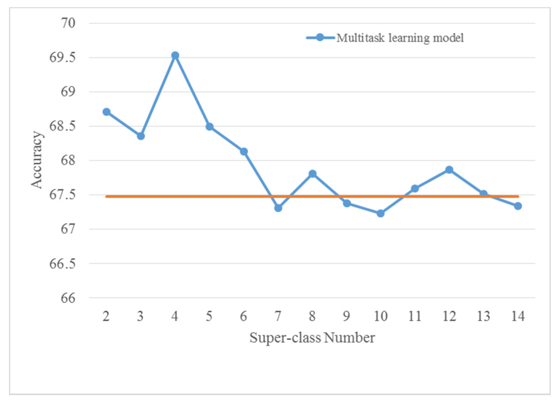
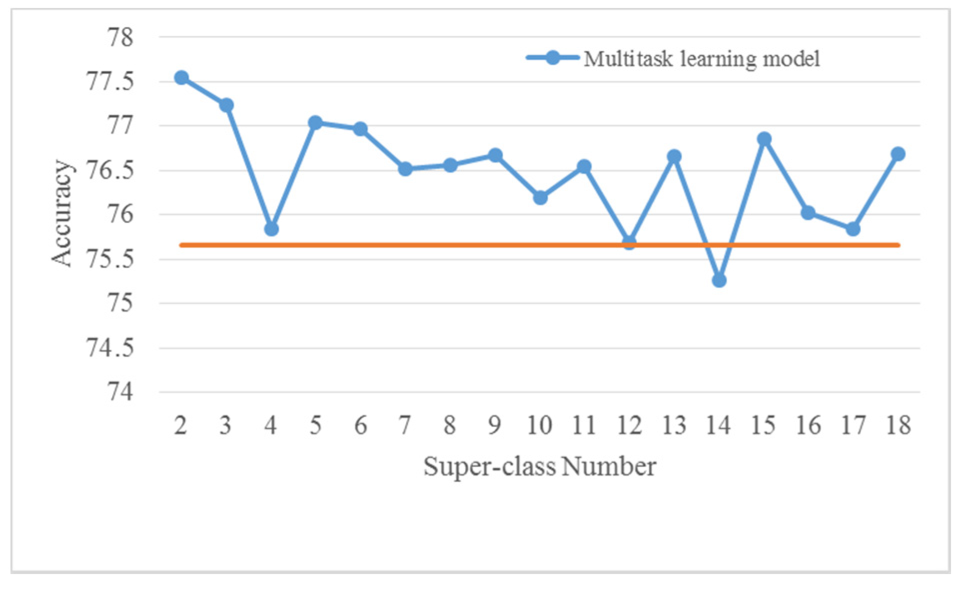
4.2. Selection of Super-Class Number
4.3. Evaluations on the TUT Acoustic Scenes 2017 Dataset
4.4. Evaluations on the LITIS Rouen Dataset
4.5. Ensemble Results
5. Discussion
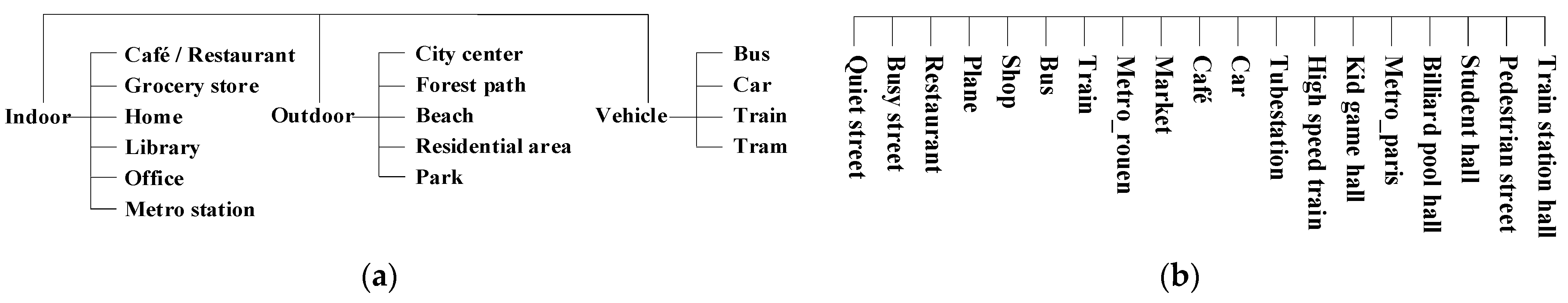
5.1. Similarity Relationship of Acoustic Scenes
5.2. Advantages of the Super-Class Construction Method
5.3. Foundation of Self-Organized Multitask Learning
5.4. Regularization by Similarity Relation
6. Conclusions
- (1)
- The similarity relation based class hierarchy construction method is effective and reasonable.
- (2)
- The constructed class hierarchy can be utilized to improve the ASC performance effectively in multitask learning.
- (3)
- For a hierarchically arranged dataset, there may exist a hierarchy that is automatically constructed by our method. This may perform better than the original hierarchy in ASC.
- (4)
- In self-organized multitask learning, the number of super-class should be chosen carefully. The multitask models with large super-class numbers would not obtain competitive results.
- (5)
- The relevance between coarse and fine-grained classes can be utilized as regularization to improve the ASC performance.
- (6)
- By arranging the class hierarchy, the self-organized multitask learning method provides a feasible way to promote the performance of a certain model.
Author Contributions
Funding
Conflicts of Interest
References
- Barchiesi, D.; Giannoulis, D.; Stowell, D.; Plumbley, M.D. Acoustic Scene Classification: Classifying environments from the sounds they produce. IEEE Signal Process. Mag. 2015, 32, 16–34. [Google Scholar] [CrossRef]
- Stowell, D.; Giannoulis, D.; Benetos, E.; Lagrange, M.; Plumbley, M.D. Detection and classification of acoustic scenes and events. IEEE Trans. Multimed. 2015, 17, 1733–1746. [Google Scholar] [CrossRef]
- Hossain, M.S.; Muhammad, G. Environment classification for urban big data using deep learning. IEEE Commun. Mag. 2018, 56, 44–50. [Google Scholar] [CrossRef]
- Imoto, K. Incorporating Intra-Class Variance to Fine-Grained Visual Recognition. Acoust. Sci. Technol. 2018, 39, 182–188. [Google Scholar] [CrossRef] [Green Version]
- Em, Y.; Gag, F.; Lou, Y.; Wang, S.; Huang, T.; Duan, L.-Y. Incorporating Intra-Class Variance to Fine-Grained Visual Recognition. In Proceedings of the 2017 IEEE International Conference on Multimedia and Expo (ICME), Hong Kong, China, 10–14 July 2017; pp. 1452–1457. [Google Scholar]
- Mesaros, A.; Heittola, T.; Diment, A.; Elizalde, B.; Shah, A.; Vincent, E.; Raj, B.; Virtanen, T. DCASE 2017 challenge setup: Tasks, datasets and baseline system. In Proceedings of the DCASE 2017-Workshop on Detection and Classification of Acoustic Scenes and Events, Munich, Germany, 16–17 November 2017; pp. 85–92. [Google Scholar]
- Ye, J.; Kobayashi, T.; Wang, X.; Tsuda, H.; Murakawa, M. Audio Data Mining for Anthropogenic Disaster Identification: An Automatic Taxonomy Approach. IEEE Trans. Emerg. Top. Comput. 2017, 8, 126–136. [Google Scholar] [CrossRef]
- Li, Y.; Liu, M.; Wang, W.; Zhang, Y.; He, Q. Acoustic Scene Clustering Using Joint Optimization of Deep Embedding Learning and Clustering Iteration. IEEE Trans. Multimed. 2019, 22, 1385–1394. [Google Scholar] [CrossRef]
- Tonami, N.; Imoto, K.; Niitsuma, M.; Yamanishi, R.; Yamashita, Y. Joint analysis of acoustic events and scenes based on multitask learning. In Proceedings of the 2019 IEEE Workshop on Applications of Signal Processing to Audio and Acoustics (WASPAA), New Paltz, NY, USA, 20–23 October 2019; pp. 338–342. [Google Scholar]
- Abrol, V.; Sharma, P. Learning Hierarchy Aware Embedding from Raw Audio for Acoustic Scene Classification. IEEE/ACM Trans. Audio Speech Lang. Process. 2020, 28, 1964–1973. [Google Scholar] [CrossRef]
- Rakotomamonjy, A.; Gasso, G. Histogram of gradients of time-frequency representations for audio scene classification. IEEE/ACM Trans. Audio Speech Lang. Process. 2014, 23, 142–153. [Google Scholar]
- Geiger, J.T.; Schuller, B.; Rigoll, G. Large-scale audio feature extraction and SVM for acoustic scene classification. In Proceedings of the 2013 IEEE Workshop on Applications of Signal Processing to Audio and Acoustics, New Paltz, NY, USA, 20–23 October 2013; pp. 1–4. [Google Scholar]
- Ma, L.; Milner, B.; Smith, D. Acoustic environment classification. ACM Trans. Speech Lang. Process. TSLP 2006, 3, 1–22. [Google Scholar] [CrossRef]
- Chakrabarty, D.; Elhilali, M. Exploring the role of temporal dynamics in acoustic scene classification. In Proceedings of the 2015 IEEE Workshop on Applications of Signal Processing to Audio and Acoustics (WASPAA), New Paltz, NY, USA, 18–21 October 2015; pp. 1–5. [Google Scholar]
- Yu, D.; Li, J. Recent progresses in deep learning based acoustic models. IEEE/CAA J. Autom. Sin. 2017, 4, 396–409. [Google Scholar] [CrossRef]
- Eghbal-Zadeh, H.; Lehner, B.; Dorfer, M.; Widmer, G. CP-JKU submission for DCASE-2016: A hybrid approach using binaural i-vectors and deep convolutional neural networks. In Proceedings of the IEEE AASP Challenge on Detection and Classification of Acoustic Scenes and Events (DCASE), Budapest, Hungary, 3 September 2016; pp. 5024–5028. [Google Scholar]
- Weiping, Z.; Jiantao, Y.; Xiaotao, X.; Xiangtao, L.; Shaohu, P. Acoustic scene classification using deep convolutional neural network and multiple spectrograms fusion. In Proceedings of the Detection and Classification of Acoustic Scenes and Events (DCASE), Munich, Germany, 16–17 November 2017; pp. 133–137. [Google Scholar]
- Xu, K.; Feng, D.; Mi, H.; Zhu, B.; Wang, D.; Zhang, L.; Cai, H.; Liu, S. Mixup-based acoustic scene classification using multi-channel convolutional neural network. In Proceedings of the Pacific Rim Conference on Multimedia, Hefei, China, 21–22 September 2018; pp. 14–23. [Google Scholar]
- Hershey, S.; Chaudhuri, S.; Ellis, D.P.; Gemmeke, J.F.; Jansen, A.; Moore, R.C.; Plakal, M.; Platt, D.; Saurous, R.A.; Seybold, B. CNN architectures for large-scale audio classification. In Proceedings of the 2017 IEEE International Conference on Acoustics, Speech and Signal Processing (ICASSP), New Orleans, LA, USA, 5–9 March 2017; pp. 131–135. [Google Scholar]
- Phan, H.; Koch, P.; Katzberg, F.; Maass, M.; Mazur, R.; Mertins, A. Audio scene classification with deep recurrent neural networks. In Proceedings of the INTERSPEECH, Stockholm, Sweden, 20–24 August 2017. [Google Scholar]
- Bae, S.H.; Choi, I.; Kim, N.S. Acoustic scene classification using parallel combination of LSTM and CNN. In Proceedings of the Detection and Classification of Acoustic Scenes and Events 2016 Workshop (DCASE2016), Budapest, Hungary, 3 September 2016; pp. 11–15. [Google Scholar]
- Xu, Y.; Huang, Q.; Wang, W.; Plumbley, M.D. Hierarchical learning for DNN-based acoustic scene classification. In Proceedings of the Detection and Classification of Acoustic Scenes and Events 2016 Workshop (DCASE2016), Budapest, Hungary, 3 September 2016; pp. 110–114. [Google Scholar]
- Guo, J.; Xu, N.; Li, L.-J.; Alwan, A. Attention based CLDNNs for short-duration acoustic scene classification. In Proceedings of the INTERSPEECH, Stockholm, Sweden, 20–24 August 2017; pp. 469–473. [Google Scholar]
- Dehak, N.; Kenny, P.J.; Dehak, R.; Dumouchel, P.; Ouellet, P. Front-end factor analysis for speaker verification. IEEE Trans. Audio Speech Lang. Process. 2010, 19, 788–798. [Google Scholar] [CrossRef]
- Hochreiter, S.; Schmidhuber, J. Long short-term memory. Neural Comput. 1997, 9, 1735–1780. [Google Scholar] [CrossRef] [PubMed]
- Zhang, X.; Zhou, F.; Lin, Y.; Zhang, S. Embedding label structures for fine-grained feature representation. In Proceedings of the IEEE Conference on Computer Vision and Pattern Recognition, Las Vegas, NV, USA, 27–30 June 2016; pp. 1114–1123. [Google Scholar]
- Sohn, K. Improved deep metric learning with multi-class n-pair loss objective. In Proceedings of the Advances in Neural Information Processing Systems, Barcelona, Spain, 5–10 December 2016; pp. 1857–1865. [Google Scholar]
- Xie, S.; Yang, T.; Wang, X.; Lin, Y. Hyper-class augmented and regularized deep learning for fine-grained image classification. In Proceedings of the IEEE Conference on Computer Vision and Pattern Recognition, Boston, MA, USA, 7–12 June 2015; pp. 2645–2654. [Google Scholar]
- Wu, H.; Merler, M.; Uceda-Sosa, R.; Smith, J.R. Learning to make better mistakes: Semantics-aware visual food recognition. In Proceedings of the 24th ACM International Conference on Multimedia, Amsterdam The Netherlands, 15–19 October 2016; pp. 172–176. [Google Scholar]
- Imoto, K.; Tonami, N.; Koizumi, Y.; Yasuda, M.; Yamanishi, R.; Yamashita, Y. Sound event detection by multitask learning of sound events and scenes with soft scene labels. In Proceedings of the ICASSP 2020–2020 IEEE International Conference on Acoustics, Speech and Signal Processing (ICASSP), Barcelona, Spain, 4–8 May 2020; pp. 621–625. [Google Scholar]
- Mun, S.; Park, S.; Han, D.K.; Ko, H. Generative adversarial network based acoustic scene training set augmentation and selection using SVM hyper-plane. In Proceedings of the DCASE 2017–Detection and Classification of Acoustic Scenes and Events Workshop, Munich, Germany, 16–17 November 2017; pp. 93–97. [Google Scholar]
- Salamon, J.; Bello, J.P. Deep convolutional neural networks and data augmentation for environmental sound classification. IEEE Signal Process. Lett. 2017, 24, 279–283. [Google Scholar] [CrossRef]
- Lu, R.; Duan, Z.; Zhang, C. Metric learning based data augmentation for environmental sound classification. In Proceedings of the 2017 IEEE Workshop on Applications of Signal Processing to Audio and Acoustics (WASPAA), New Paltz, NY, USA, 15–18 October 2017; pp. 1–5. [Google Scholar]
- Goodfellow, I.; Pouget-Abadie, J.; Mirza, M.; Xu, B.; Warde-Farley, D.; Ozair, S.; Courville, A.; Bengio, Y. Generative Adversarial Networks. Proc. Adv. Neural Inf. Process. Syst. 2014, 3, 2672–2680. [Google Scholar] [CrossRef]
- Zhong, Z.; Zheng, L.; Kang, G.; Li, S.; Yang, Y. Random Erasing Data Augmentation. AAAI 2020, 34, 13001–13008. [Google Scholar] [CrossRef]
- Gharib, S.; Derrar, H.; Niizumi, D.; Senttula, T.; Tommola, J.; Heittola, T.; Virtanen, T.; Huttunen, H. Acoustic scene classification: A competition review. In Proceedings of the 2018 IEEE 28th International Workshop on Machine Learning for Signal Processing (MLSP), Aalborg, Denmark, 17–20 September 2018; pp. 1–6. [Google Scholar]
- Zhang, H.; Cisse, M.; Dauphin, Y.N.; Lopez-Paz, D. Mixup: Beyond empirical risk minimization. In Proceedings of the International Conference on Learning Representations, Vancouver, BC, Canada, 30 April–3 May 2018. [Google Scholar]
- Nawa, S.; Quatieri, T.; Lim, J. Signal Reconstruction from Short-Time Fourier Transform Magnitude. IEEE Trans. Acoust. Speech Signal Process. 1983, 31, 986–998. [Google Scholar]
- Brown, C.J.; Puckette, S.M. An efficient algorithm for the calculation of a constant Q transform. J. Acoust. Soc. Am. 1992, 92, 2698–2701. [Google Scholar] [CrossRef] [Green Version]
- Logan, B. Mel frequency cepstral coefficients for music modeling. In Proceedings of the In International Symposium on Music Information Retrieval, Montréal, QC, Canada, 23–25 October 2000; pp. 1–11. [Google Scholar]
- Boashash, B.; Khan, N.A.; Ben-Jabeur, T. Time-frequency features for pattern recognition using high-resolution TFDs: A tutorial review. Digit. Signal Process. 2015, 40, 1–30. [Google Scholar] [CrossRef]
- Paseddula, C.; Gangashetty, S.V. Late fusion framework for Acoustic Scene Classification using LPCC, SCMC, and log-Mel band energies with Deep Neural Networks. Appl. Acoust. 2021, 172, 107568. [Google Scholar] [CrossRef]
- Mcdonnellk, M.D.; Gao, W. Acoustic Scene Classification Using Deep Residual Networks with Late Fusion of Separated High and Low Frequency Paths. In Proceedings of the ICASSP 2020–2020 IEEE International Conference on Acoustics, Speech and Signal Processing (ICASSP), Virtual Conference, 4–8 May 2020; pp. 141–145. [Google Scholar]
- Ng, A.; Jordan, M.; Weiss, Y. On spectral clustering: Analysis and an algorithm. In Advances in Neural Information Processing Systems; MIT Press: Cambridge, MA, USA, 2002; pp. 849–856. [Google Scholar]
- Gopal, S.; Yang, Y. Recursive regularization for large-scale classification with hierarchical and graphical dependencies. In Proceedings of the 19th ACM SIGKDD–International Conference on Knowledge Discovery and Data Mining, Chicago, IL, USA 11–14 August 2013; pp. 257–265. [Google Scholar]
- He, K.; Zhang, X.; Ren, S.; Sun, J. Deep residual learning for image recognition. In Proceedings of the IEEE Conference on Computer Vision and Pattern Recognition, Las Vegas, NV, USA, 27–30 June 2016; pp. 770–778. [Google Scholar]
- Szegedy, C.; Liu, W.; Jia, Y.; Sermanet, P.; Reed, S.; Anguelov, D.; Erhan, D.; Vanhoucke, V.; Rabinovich, A. Going deeper with convolutions. In Proceedings of the IEEE Conference on Computer Vision and Pattern Recognition, Boston, MA, USA, 7–12 June 2015; pp. 1–9. [Google Scholar]
- Rakotomamonjy, A. Supervised representation learning for audio scene classification. IEEE/ACM Trans. Audio Speech Lang. Process. 2017, 25, 1253–1265. [Google Scholar] [CrossRef]
- Abadi, M.; Agarwal, A.; Barham, P.; Barham, P.; Brevdo, E.; Chen, Z.; Corrado, G.S.; Davis, A.; Dean, J.; Devin, M.; et al. TensorFlow: Large-scale machine learning on heterogeneous systems. In Proceedings of the Operating Systems Design and Implementation, Savannah, GA, USA, 2–4 November 2016; pp. 265–283. [Google Scholar]
- Kingma, D.P.; Ba, J. Adam: A method for stochastic optimization. In Proceedings of the International Conference on Learning Representations, San Diego, CA, USA, 7–9 May 2015; pp. 1–15. [Google Scholar]
- Han, Y.; Park, J.; Lee, K. Convolutional neural networks with binaural representations and background subtraction for acoustic scene classification. In Proceedings of the DCASE 2017–Detection and Classification of Acoustic Scenes and Events Workshop, Munich, Germany, 16–17 November 2017; pp. 46–50. [Google Scholar]
- Alamir, M.A. A novel acoustic scene classification model using the late fusion of convolutional neural networks and different ensemble classifiers. Appl. Acoust. 2021, 175, 107829. [Google Scholar] [CrossRef]
- Chen, H.; Zhang, P.; Yan, Y. An audio scene classification framework with embedded filters and a DCT-based temporal module. In Proceedings of the ICASSP 2019–2019 IEEE International Conference on Acoustics, Speech and Signal Processing (ICASSP), Brighton, UK, 12–17 May 2019; pp. 835–839. [Google Scholar]
- Wu, Y.; Lee, T. Enhancing sound texture in CNN-based acoustic scene classification. In Proceedings of the ICASSP 2019–2019 IEEE International Conference on Acoustics, Speech and Signal Processing (ICASSP), Brighton, UK, 12–17 May 2019; pp. 815–819. [Google Scholar]
- Pham, L.; Phan, H.; Nguyen, T.; Palaniappan, R.; Mertins, A.; McLoughlin, I. Robust acoustic scene classification using a multi-spectrogram encoder-decoder framework. Digit. Signal Process. 2021, 110, 102943. [Google Scholar] [CrossRef]
- Lee, Y.J.; Grauman, K. Learning the easy things first: Self-paced visual category discovery. In Proceedings of the IEEE Conference on Computer Vision and Pattern Recognition, Colorado Springs, CO, USA, 20–25 June 2011; pp. 1721–1728. [Google Scholar]
- Caruana, R. Multitask learning. Mach. Learn. 1997, 28, 41–75. [Google Scholar] [CrossRef]


| Layer | Conv1 | Conv2 | Pool1 | Conv3 | Conv4 | Pool2 | Conv5 | Conv6 | Conv7 | Conv8 | Pool3 | Conv9 | Conv10 | Conv11 | Full1 |
|---|---|---|---|---|---|---|---|---|---|---|---|---|---|---|---|
| Kernel | 5 × 5 | 3 × 3 | Max, 2 × 2 | 3 × 3 | 3 × 3 | Max, 2 × 2 | 3 × 3 | 3 × 3 | 3 × 3 | 3 × 3 | Max, 2 × 2 | 3 × 3 | 1 × 1 | 1 × 1 | − |
| Stride | 2 | 1 | 2 | 1 | 1 | 2 | 1 | 1 | 1 | 1 | 2 | 1 | 1 | 1 | − |
| Padding | 2 | 1 | 0 | 1 | 1 | 0 | 1 | 1 | 1 | 1 | 0 | 0 | 0 | 0 | − |
| Number of Channels | 32 | 32 | 32 | 64 | 64 | 64 | 128 | 128 | 128 | 128 | 128 | 512 | 512 | C | C |
| Dropout rate | − | − | 0.3 | − | − | 0.3 | − | − | − | − | 0.3 | 0.5 | 0.5 | − | − |
| Activation | ReLu | ReLu | − | ReLu | ReLu | − | ReLu | ReLu | ReLu | ReLu | − | ReLu | ReLu | ReLu | − |
| Batchnorm | Yes | Yes | − | Yes | Yes | − | Yes | Yes | Yes | Yes | − | Yes | Yes | Yes | − |
| Clustering Scheme | Supper-Class for STFT Model | Supper-Class for CQT Model | Supper-Class for Log-Mel Model |
|---|---|---|---|
| Two Super-Classes | 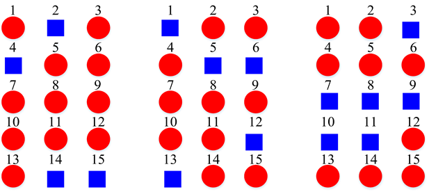 | ||
| Three Super-Classes | 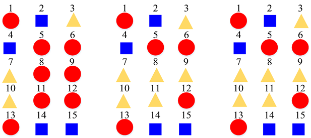 | ||
| Four Super-Classes |  | ||
| Five Super-Classes | 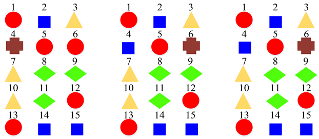 | ||
| Six Super-Classes | 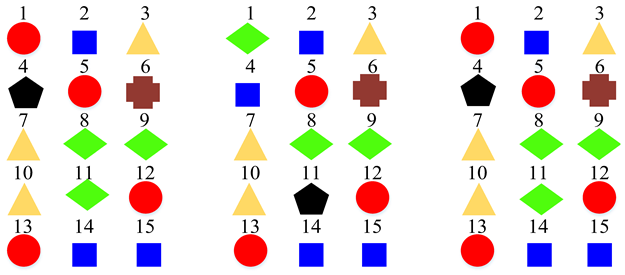 | ||
| Model Type | Feature Type | Super-Class Number | 15 Scenes Accuracy | Super-Class Accuracy |
|---|---|---|---|---|
| Basic Model | STFT | / | 60.0 ± 0.5 | / |
| Multitask | STFT | 2 | 61.1 ± 0.3 | 93.1 ± 0.6 |
| Multitask | STFT | 3 | 62.0 ± 0.1 | 88.8 ± 0.4 |
| Multitask | STFT | 4 | 61.1 ± 0.1 | 85.9 ± 0.8 |
| Multitask | STFT | 5 | 61.5 ± 0.5 | 82.6 ± 0.2 |
| Multitask | STFT | 6 | 60.7 ± 0.2 | 77.0 ± 0.2 |
| Basic Model | CQT | / | 67.5 ± 0.2 | / |
| Multitask | CQT | 2 | 68.7 ± 0.2 | 96.2 ± 0.1 |
| Multitask | CQT | 3 | 68.4 ± 0.3 | 92.5 ± 0.4 |
| Multitask | CQT | 4 | 69.5 ± 0.8 | 89.3 ± 0.7 |
| Multitask | CQT | 5 | 68.5 ± 0.4 | 84.8 ± 0.4 |
| Multitask | CQT | 6 | 68.1 ± 0.6 | 84.0 ± 0.6 |
| Basic Model | log-Mel | / | 69.3 ± 0.1 | / |
| Multitask | log-Mel | 2 | 71.5 ± 1.0 | 94.9 ± 0.1 |
| Multitask | log-Mel | 3 | 72.1 ± 0.4 | 93.8 ± 0.1 |
| Multitask | log-Mel | 4 | 71.5 ± 1.5 | 91.0 ± 0.4 |
| Multitask | log-Mel | 5 | 72.8 ± 0.7 | 89.5 ± 0.5 |
| Multitask | log-Mel | 6 | 71.9 ± 1.1 | 85.2 ± 0.8 |
| Clustering Scheme | Generated by STFT Model | Generated by CQT Model | Generated by Log-Mel Model |
|---|---|---|---|
| Two Super-Classes | 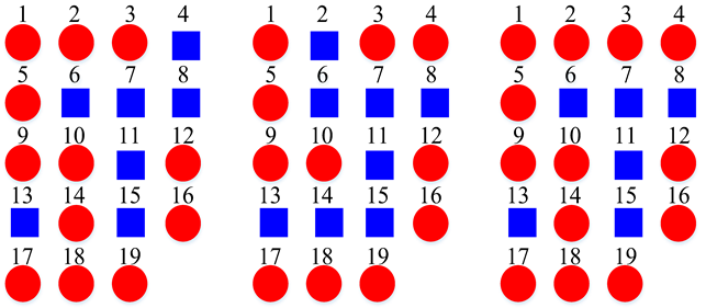 | ||
| Three Super-Classes | 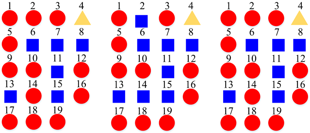 | ||
| Four Super-Classes | 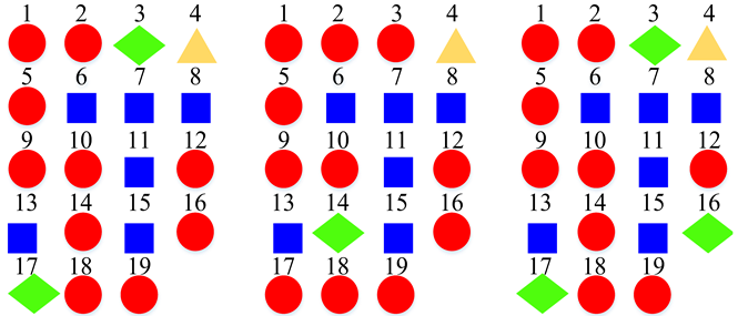 | ||
| Five Super-Classes | 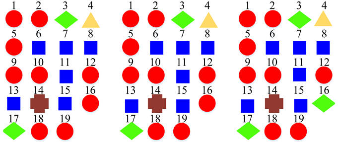 | ||
| Six Super-Classes | 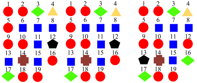 | ||
| Model Type | Feature Type | Super-Class Number | 19 Scenes Accuracy | Super-Class Accuracy |
|---|---|---|---|---|
| Basic Model | STFT | / | 74.4 ± 0.7 | / |
| Multitask | STFT | 2 | 75.7 ± 0.6 | 97.1 ± 0.2 |
| Multitask | STFT | 3 | 75.0 ± 0.6 | 96.6 ± 0.2 |
| Multitask | STFT | 4 | 76.0 ± 0.4 | 95.8 ± 0.3 |
| Multitask | STFT | 5 | 75.5 ± 0.9 | 96.1 ± 0.1 |
| Multitask | STFT | 6 | 74.7 ± 0.5 | 95.2 ± 0.3 |
| Basic Model | CQT | / | 75.6 ± 0.8 | / |
| Multitask | CQT | 2 | 77.5 ± 0.4 | 97.3 ± 0.1 |
| Multitask | CQT | 3 | 77.2 ± 0.5 | 97.7 ± 0.4 |
| Multitask | CQT | 4 | 75.8 ± 0.7 | 96.6 ± 0.0 |
| Multitask | CQT | 5 | 77.0 ± 0.3 | 96.7 ± 0.2 |
| Multitask | CQT | 6 | 76.5 ± 0.6 | 95.1 ± 0.3 |
| Basic Model | log-Mel | / | 76.3 ± 0.7 | / |
| Multitask | log-Mel | 2 | 78.1 ± 0.3 | 97.9 ± 0.3 |
| Multitask | log-Mel | 3 | 77.7 ± 0.9 | 97.9 ± 0.0 |
| Multitask | log-Mel | 4 | 76.2 ± 0.7 | 95.6 ± 0.3 |
| Multitask | log-Mel | 5 | 76.7 ± 0.3 | 95.6 ± 0.2 |
| Multitask | log-Mel | 6 | 77.1 ± 1.0 | 94.9 ± 0.4 |
| Reference | Method | Accuracy | Dataset |
|---|---|---|---|
| [31] | GAN + SVM + FCNN | 83.3 | TUT |
| [51] | Background subtraction | 80.4 | TUT |
| [52] | Late fusion of CNN and ensemble classifiers | 80.0 | TUT |
| [53] | Embedded filters + DCT-based temporal module | 79.2 | TUT |
| [17] | Multi-spectrogram fusion | 77.7 | TUT |
| [18] | Mixup + multi-channel | 76.7 | TUT |
| [54] | Sound texture enhancement | 75.7 | TUT |
| [55] | Multi-spectrogram encoder-decoder | 72.6 | TUT |
| Ensemble of three basic models | Ensemble | 77.8 | TUT |
| Our method | Super-class construction + multitask learning | 81.4 | TUT |
| [48] | Supervised nonnegative matrix factorization | 81.8 | Rouen-15 |
| Ensemble of three basic models | Ensemble | 78.1 | Rouen-revised |
| Our method | Super-class construction + multitask learning | 83.9 | Rouen-revised |
Publisher’s Note: MDPI stays neutral with regard to jurisdictional claims in published maps and institutional affiliations. |
© 2021 by the authors. Licensee MDPI, Basel, Switzerland. This article is an open access article distributed under the terms and conditions of the Creative Commons Attribution (CC BY) license (https://creativecommons.org/licenses/by/4.0/).
Share and Cite
Zheng, W.; Mo, Z.; Zhao, G. Clustering by Errors: A Self-Organized Multitask Learning Method for Acoustic Scene Classification. Sensors 2022, 22, 36. https://doi.org/10.3390/s22010036
Zheng W, Mo Z, Zhao G. Clustering by Errors: A Self-Organized Multitask Learning Method for Acoustic Scene Classification. Sensors. 2022; 22(1):36. https://doi.org/10.3390/s22010036
Chicago/Turabian StyleZheng, Weiping, Zhenyao Mo, and Gansen Zhao. 2022. "Clustering by Errors: A Self-Organized Multitask Learning Method for Acoustic Scene Classification" Sensors 22, no. 1: 36. https://doi.org/10.3390/s22010036
APA StyleZheng, W., Mo, Z., & Zhao, G. (2022). Clustering by Errors: A Self-Organized Multitask Learning Method for Acoustic Scene Classification. Sensors, 22(1), 36. https://doi.org/10.3390/s22010036